Quantum annealing: An introduction and new developments

Abstract

Quantum annealing is a generic algorithm using quantum-mechanical fluctuations to search for the solution of an optimization problem. The present paper first reviews the fundamentals of quantum annealing and then reports on preliminary results for an alternative method. The review part includes the relationship of quantum annealing with classical simulated annealing. We next propose a novel quantum algorithm which might be available for hard optimization problems by using a classical-quantum mapping as well as the Jarzynski equality introduced in nonequilibrium statistical physics.

I Introduction

Recent remarkable advances in experimental techniques have enabled us to fabricate dedicated nanostructures, in which prominent quantum effects are observed and/or controlled. Such technological achievements open up the possibilities of realization of advanced methods of quantum computation. In this article, we review and present new developments in quantum annealing (QA) QA1 ; QA2 ; QA3 ; QA4 ; QA5 ; QA6 ; QA as an important subfield of quantum computation.

Quantum annealing is a generic algorithm intended for solving optimization problems by use of quantum tunneling. An optimization problem is formulated as a task to minimize a real single-valued function, called a cost function, of multivariables. We will in particular be interested in combinatorial optimization problems, in which variables assume discrete values OP1 ; OP2 . We will use the simple term of “an optimization problem” to mean a combinatorial optimization problem.

Optimization problems are classified roughly into two types, easy and hard ones. They are distinguished by the computational cost to solve optimization problems. Easy problems are those which can be solved by the best algorithms in time polynomial in the problem size (polynomial complexity). For hard problems, in contrast, the best known algorithms cost exponentially long time as a function of the system size (exponential complexity). For these latter problems, it is virtually impossible to find the optimal solution in a reasonable time, if the problem size exceeds a moderate value. Most of the interesting optimization problems belong to the latter hard class. It is thus important practically to devise algorithms which give approximate but accurate solutions efficiently.

One of the generic algorithms proposed as part of such efforts is QA. This is a method to use quantum dynamics and quantum tunneling effects to let the system explore the phase space toward the solution of an optimization problem. Quantum adiabatic evolution (or quantum adiabatic computation) shares essentially the same idea Farhi .

A related algorithm of simulated annealing (SA) is widely used in practice to solve optimization problems approximately in a reasonable time SA1 ; SA2 . In SA, the cost function to be minimized is identified with the energy of a classical statistical-mechanical system. The system is then given a temperature, as an artificial control parameter. By decreasing the parameter slowly from a high value to zero, one hopes to drive the system to the state with the lowest value of the energy. The idea is that the system is expected to stay close to thermal equilibrium during the protocol in SA. If the rate of decrease in temperature is sufficiently slow, the system will be led in the end to the zero-temperature equilibrium state, the lowest-energy state. SA is thus regarded as an algorithm to make use of (non-)equilibrium statistical mechanics for an efficient exploration of the phase space.

Let us turn our attention to QA, which is the main topic of this article. In SA, we make use of thermal, classical, fluctuations to introduce a stochastic search for the desired lowest-energy state by allowing the system to hop from state to state over intermediate energy barriers. In QA, by contrast, we introduce non-commutative operators as artificial degrees of freedom of quantum nature. They induce quantum fluctuations. We first set the strength of quantum fluctuations to a very large value to search for the global structure of the phase space, similarly to the high-temperature situation in SA. Then the strength is gradually decreased to finally vanish to recover the original system hopefully in the lowest-energy state. Quantum tunneling between different classical states replaces thermal hopping in SA.

An observant reader should have noticed a number of similarities and differences between SA and QA. In both methods, we have to control the relevant parameters slowly and carefully to tune the strengths of thermal or quantum fluctuations as desired. The idea behind QA is to keep the system close to the instantaneous ground state of a quantum system. This aspect is analogous to the protocol of SA, in which one tries to keep the system state in quasi-equilibrium. It is indeed possible to render this analogy into a more precise formulation, from which several important developments have been achieved. An example of such cases will be explained later.

Let us move our attention to some of the developments in nonequilibrium statistical physics. Several exact relations between nonequilibrium processes and equilibrium states have been derived. The Jarzynski equality (JE) is one of such remarkable results JE1 ; JE2 . This equality states that we can reproduce useful information on equilibrium states from data obtained by the repetition of non-equilibrium processes. We first prepare an ensemble of states consisting of equilibrium distribution. We then drive these states by tuning some parameters following a predetermined schedule. In general the system during this process cannot be kept in equilibrium. However, the average with weights given by the exponentiated value of the work done during the nonequilibrium process coincides with the thermal average of the exponential of free energy difference between the final and initial states in equilibrium. The state is not necessarily kept in equilibrium also during the protocol of SA as mentioned above. However, JE tells us the possibility to obtain information of equilibrium state from nonequilibrium processes. Indeed, the application of JE to SA has been studied by several researchers NJ ; Iba ; Pop1 ; ON1 ; ON2 . This application is known to successfully extract information on the equilibrium state faster than the ordinary procedure of SA with the aid of the property of JE. We show a quantum version of the algorithm with JE in this article.

The present paper consists of five sections. In §2, we review the foundation of QA. In the following section, we introduce the classical-quantum mapping. Here we understand the property of SA from the point of view of quantum mechanics. Then, we construct an algorithm of QA with JE in §4. The last section presents a summary.

II Quantum annealing

Suppose that the optimization problem we wish to solve has been formulated as the minimization of a cost function, which we regard as a Hamiltonian $H_{0}$ of a classical many-body system. As a simple example, let us consider the problem of database search to find a specific item among $N$ items. If the specific item to be found is denoted by a bracket $|\Psi_{0}\rangle$, the cost function to be minimized is simply written as

$$H_{0}=I-|\Psi_{0}\rangle\langle\Psi_{0}|,$$ (1)

where $I$ is the $N$-dimensional identity matrix.

II.1 Algorithm of QA

In QA, we use quantum fluctuations to search the ground state of $H_{0}$. To this end we introduce an operator $H_{1}$, which does not commute with $H_{0}$. The whole quantum system is then expressed as

$$H(t)=\frac{t}{\tau}H_{0}+\left(1-\frac{t}{\tau}\right)H_{1},$$ (2)

where $\tau$ is the computation time and is an important parameter in the following discussions. The initial Hamiltonian is set as $H(0)=H_{1}$ and the final system is described by $H(\tau)=H_{0}$. It is crucial to prepare an appropriate Hamiltonian $H_{1}$, whose ground state is trivially found. For instance, we prepare $H_{1}$ with the following form,

$$H_{1}=I-|\Phi_{0}\rangle\langle\Phi_{0}|,$$ (3)

where

$$|\Phi_{0}\rangle=\frac{1}{\sqrt{N}}\sum_{j=1}|j\rangle.$$ (4)

Its ground state is trivially given by a linear combination of all states with a uniform weight.

The optimization protocol by QA is to start the algorithm from the preparation of the ground state of $H_{1}$ as the initial state. The whole system is then driven by the time-dependent Hamiltonian $H(t)$ following the Schrödinger equation. If we choose a very large value of $\tau$, the system evolves slowly. Such a slow time evolution would let the system closely follow the instantaneous ground state of the total Hamiltonian $H(t)$ if the condition set by the adiabatic theorem is satisfied.

II.2 Adiabatic evolution

Let us formulate the above statement more precisely. For a sufficiently large $\tau$, the adiabatic theorem guarantees that the state at time $t$, $|\psi(t)\rangle$, is very close to the instantaneous ground state $|0(t)\rangle$, $|\langle 0(t)|\psi(t)\rangle|\approx 1$, if the following condition is satisfied, in consideration that the protocol of QA starts from the initial ground state. We assume that the instantaneous ground state $|0(t)\rangle$ is non-degenerate. If we write the instantaneous first excited state and its energy as $|1(t)\rangle$ and $E_{1}(t)$, respectively, the quantum adiabatic theorem states that condition for $|\langle 0(t)|\psi(t)\rangle|^{2}=1-\epsilon^{2}$ ($\epsilon\ll 1$) to hold is given by

$$\frac{\mathrm{max}\left|\langle 1(t)|\displaystyle\frac{dH(t)}{dt}|0(t)\rangle\right|}{\mathrm{min}\Delta(t)^{2}}=\epsilon,$$ (5)

where max and min are evaluated between $t=0$ and $t=\tau$ and $\Delta(t)$ is the energy gap, $\Delta(t)=E_{1}(t)-E_{0}(t)$ with $E_{0}(t)$ being the instantaneous ground-state energy. For our case of Eq. (2), the numerator of Eq. (5) with the time derivative of $H(t)$ is proportional to $1/\tau$. Therefore the adiabatic condition of QA is written as

$$\tau\propto\frac{1}{\epsilon~{}\mathrm{min}\Delta(t)^{2}}.$$ (6)

If we choose $\tau$ large enough to satisfy this condition, we can obtain the ground state of $H_{0}$ at $t=\tau$ with a high probability. A serious problem arises if the energy gap $\Delta(t)$ collapses as the system size increases because then the computation time $\tau$ increases according to Eq. (6). Also the requirement of a small error probability $\epsilon$ pushes $\tau$ to a larger value.

We can evaluate the computation time of the database search problem by QA using Eqs. (1)-(4) GloG . The energy gap is given by

$$\Delta(t)=\sqrt{1-\frac{1}{4}\left(1-\frac{1}{N}\right)\frac{t}{\tau}\left(1-\frac{t}{\tau}\right)}.$$ (7)

Its minimum is $\mathrm{min}\Delta(\tau/2)=1/\sqrt{N}$. Therefore the computation time is proportional to $N$. This is essentially the same as the simple serial search. However, if we control the system evolution slowly around $t=\tau/2$, where the gap assumes its minimum, than at other time, then the transition to excited states is likely to be suppressed and the probability of success may increase. More explicitly, the time dependence of the Hamiltonian is chosen to involve a monotonically increasing function $f(t)$, instead of the simple $t/\tau$ and $1-t/\tau$ in Eq. (2), as

$$H(t)=f(t)H_{0}+\left\{1-f(t)\right\}H_{1}.$$ (8)

Then we demand that the adiabatic condition of Eq. (5), without the ‘max’ and ‘min’ operations, is satisfied at each time $t$. The result is a differential equation for $f(t)$, by solving which we achieve the optimal control of the dynamics. It actually turns out that the total time evolution obtained by this method is proportional to $\sqrt{N}$. This is a significant improvement over the above-mentioned simple result $\tau\propto N$. This is equivalent to the computation time of the Grover algorithm Grover . This is an explicit, remarkable example in which quantum effects accelerate the convergence toward the optimal solution. It has been established in many other cases by numerical and analytical methods that QA achieves superior performance compared with SA CT . Also known is a convergence theorem of QA CT : It is guaranteed that the system converges to the optimal solution after an infinite time of evolution if an appropriate control of a system parameter is chosen. This is to be compared with a convergence theorem for SA GG , where the time control of the system parameter (temperature) is constrained to be slower than the corresponding one in QA.

II.3 Errors in QA

Although the convergence of QA to the optimal solution is guaranteed in the infinite-time limit as mentioned above, we have to carry out the computation in a finite time $\tau$. It is therefore important to estimate how the error, the probability not to reach the optimal state, depends upon $\tau$. The adiabatic theorem provides an answer to this question: The error after an adiabatic evolution of $\tau$ is generically proportional to $\tau^{-2}$ in the limit of large $\tau$ as long as the system size $N$ is kept finite SO . However, if the system size grows, the energy gap $\Delta(t)$ becomes small and eventually collapses to zero as $N\to\infty$ when a quantum phase transition takes place. Thus the study of quantum phase transitions is an important part of the analyses of QA.

For instance, how the error in QA depends on the complexity of the optimization problems is interesting in order to understand the performance of QA. The errors in the final state after the process of QA can be regarded as imperfections or defects in the state caused by the evolution across a phase transition. The dynamics across a phase transition is well understood via the Kibble-Zurek mechanism KZ1 ; KZ2 . This aspect of error evaluation has been attracting increasing attention KZ3 ; KZ4 ; KZ5 ; KZ6 ; KZ7 .

II.4 Hard optimization problems

A hard optimization problem is often represented in QA in terms of a Hamiltonian $H(t)$ with a phase transition accompanying an exponentially small energy gap $\propto\exp(-\alpha N)~{}(\alpha>0)$. One of the examples is found in the random energy model REM . Consider the Hamiltonian

$$H_{0}=-\sum_{\{i_{p}\}}J_{i_{1},i_{2},\cdots,i_{p}}\sigma_{i_{1}}^{z}\sigma_{i_{2}}^{z}\cdots\sigma_{i_{p}}^{z},$$ (9)

where the summation is taken over all combinations of $p$ sites among $N$ of them, and $\sigma_{i}^{z}$ is the $z$ component of a Pauli spin operator at site $i$. The interaction $J_{i_{1},i_{2},\cdots,i_{p}}$ follows the Gaussian distribution with a vanishing mean and variance $p!/(2N^{p-1})$, which guarantees a sensible thermodynamic limit for any $p$ including the limit $p\to\infty$. The random energy model is defined as the limit $p\to\infty$ of the Hamiltonian (9). This limit significantly simplifies the problem. In particular the energy spectrum turns out to obey the Gaussian distribution with vanishing mean and variance $\sqrt{N/2}$. Any energy level takes a value drawn from this distribution independently of other levels.

Let us consider to find the ground state of the random energy model by QA. The transverse-field operator is often used as quantum fluctuations for searching the ground state in spin glasses including the random energy model,

$$H_{1}=-\sum_{i}\sigma_{i}^{x}.$$ (10)

Quantum annealing of the random energy model has the ground state of $H_{1}$ as the initial state, which is trivially given as $|\Psi(0)\rangle=\sum_{\{\sigma\}}|\sigma\rangle/{\sqrt{2}^{N}}$, where $\sigma_{i}$ is an eigenvalue of $\sigma_{i}^{z}$. By a perturbation theory, we can evaluate the asymptotic behavior of the minimum energy gap of the random energy model with a transverse field as $\Delta\propto\exp(-\alpha N)$ for a sufficiently large system size $N$ FT . Therefore the adiabatic theorem states that QA, as long as one demands the system to stay arbitrarily close to the instantaneous ground state, does not work in a time polynomial in system size.

We introduce another instance from one of the famous combinatorial optimization problems, the exact cover. This is a special version of constraint satisfaction problems. Let us consider $N$ spins and $M$ “clauses”, each one of which involves three Ising spins chosen at random. The energy of a clause is zero if one spin is $-1$ and the other two are $1$. Otherwise, the energy is defined as 1. This assignment of the energy is realized by an Ising model as

$$H_{0} = \frac{1}{8}\sum_{m=1}^{M}\left(\sigma_{m_{1}}^{z}\sigma_{m_{2}}^{z}\sigma_{m_{3}}^{z}-\sigma_{m_{1}}^{z}-\sigma_{m_{2}}^{z}-\sigma_{m_{3}}^{z}\right.$$

$$\quad\left.+\sigma_{m_{1}}^{z}\sigma_{m_{2}}^{z}+\sigma_{m_{2}}^{z}\sigma_{m_{3}}^{z}+\sigma_{m_{3}}^{z}\sigma_{m_{1}}^{z}+5\right).$$

Numerical simulations have shown that the minimum energy gap during QA of the exact cover has the asymptotic form proportional to $\exp(-\alpha N)$ FT2 ; FT3 . Thus we again encounter a similar problem to the random energy model.

The behavior of the energy gap as $\exp(-\alpha N)$ is characteristic of first-order phase transitions in quantum systems. Therefore the problem concerning the bottleneck of QA appears even in the simple ferromagnetic model, namely the Ising model with three-body interaction FT4 . This model also exhibits a first-order phase transition with an exponentially small gap. This fact may be taken as an indication that QA would fail to find a trivial ground state in a reasonable time. However we have some room in the choice of quantum fluctuations expressed by $H_{1}$. It remains to see if an appropriate choice of the quantum term $H_{1}$ can help us avoid these difficulties in the framework of QA under the constraint of an adiabatic evolution.

In the rest of this article, we provide a different approach to overcome the difficulty of the energy gap closure based on a different idea.

III Classical-quantum mapping

The analogy between QA and SA can be pursued in a systematic manner by the exploitation of an ingenious mapping between a classical thermal state and a corresponding quantum state QC . This mapping is different from the conventional quantum-classical mapping in terms of the Suzuki-Trotter formula or the path integral formulation. In particular, the same spatial dimensionality is shared by classical and quantum systems according to the present mapping.

III.1 Mapping of a classical system to a quantum system

In order to formulate the classical-quantum mapping, we consider a classical Ising spin system with a configuration $\sigma$. This system is assumed to obey a stochastic dynamics described by the master equation

$$\frac{d}{dt}P(\sigma;t)=\sum_{\sigma^{\prime}}M(\sigma|\sigma^{\prime};t)P(\sigma^{\prime};t),$$ (12)

where $M(\sigma^{\prime}|\sigma;t)$ expresses the transition matrix satisfying the detailed balance condition

$$M(\sigma|\sigma^{\prime};t)\tilde{P}(\sigma^{\prime})=M(\sigma^{\prime}|\sigma;t)\tilde{P}(\sigma).$$ (13)

The instantaneous equilibrium distribution $e^{-\beta(t)H_{0}(\sigma)}/Z(t)$ is denoted as $\tilde{P}(\sigma;t)$. Since we are considering a dynamic control of the temperature, $T(t)$, the time variable $t$ has been written explicitly in the arguments of the inverse temperature and the partition function.

The (instantaneous) equilibrium state of the above stochastic dynamics is now shown to be expressed as the ground state of a quantum Hamiltonian. A general form of such a quantum Hamiltonian is given as

$$H_{q}(\sigma^{\prime}|\sigma;t)=\delta_{\sigma^{\prime},\sigma}-\mathrm{e}^{\beta(t)H_{0}(\sigma^{\prime})/2}M(\sigma^{\prime}|\sigma;t)\mathrm{e}^{-\beta(t)H_{0}(\sigma)/2}.$$ (14)

This Hamiltonian has the following state as its ground state,

$$|\Psi_{\mathrm{eq}}(t)\rangle=\frac{1}{\sqrt{Z(t)}}\sum_{\sigma}\mathrm{e}^{-\frac{\beta(t)}{2}H_{0}(\sigma)}|\sigma\rangle.$$ (15)

It is clear that the quantum expectation value of a physical quantity $A(\sigma)$ by $|\Psi_{\mathrm{eq}}(t)\rangle$ coincides with the thermal expectation value of the same quantity. The ground state energy for this ground state is $0$, which is shown by the detailed-balance condition,

$$\left(\delta_{\sigma^{\prime},\sigma}-\mathrm{e}^{\frac{\beta(t)}{2}H_{0}(\sigma^{\prime})}M(\sigma^{\prime}|\sigma;t)\mathrm{e}^{-\frac{\beta(t)}{2}H_{0}(\sigma)}\right)|\Psi_{\mathrm{eq}}(t)\rangle$$

$$\propto\sum_{\sigma}\left(\mathrm{e}^{-\frac{\beta(t)}{2}H_{0}(\sigma^{\prime})}-\mathrm{e}^{\frac{-\beta(t)}{2}H_{0}(\sigma^{\prime})}M(\sigma|\sigma^{\prime};t)\right)|\sigma\rangle$$

$$=0,$$ (16)

where we used the detailed balance condition and the requirement for conservation of probability $\sum_{\sigma}M(\sigma|\sigma^{\prime};t)|\sigma\rangle=|\sigma^{\prime}\rangle$. The excited states have positive-definite eigenvalues, which can be confirmed by the application of the Perron-Frobenius theorem. By using the above special quantum system, we can treat a quasi-equilibrium stochastic process in SA as an adiabatic quantum-mechanical dynamics in QA. The stochastic dynamics can be mapped into the quantum dynamics as above introduced even for the system with continuous variables by focusing the relationship between the Fokker-Planck equation and the Shrödinger equation Orland .

III.2 Similarity of SA and QA

Let us consider an optimization problem that can be expressed as a Hamiltonian with local interactions

$$H_{0}=\sum_{j}H_{j},$$ (17)

where $H_{j}$ involves $\sigma_{j}^{z}$ and a finite number of $\sigma_{k}^{z}~{}(k\neq j)$. A simple instance is a system with nearest-neighbor interactions,

$$H_{j}=-\sum_{k\in j}J_{jk}\sigma_{j}^{z}\sigma_{k}^{z},$$ (18)

where $k$ is a site neighboring to $j$. The following explicit choice of the quantum Hamiltonian as an example of Eq. (14) facilitates our analysis,

$$H_{q}^{\mathrm{SG}}(t)=-\chi(t)\sum_{j}\left(\sigma_{j}^{x}-\mathrm{e}^{\frac{\beta(t)}{2}H_{j}}\right),$$ (19)

where $\chi(t)=e^{-\beta(t)p}$ with $p=\mathrm{max}_{i}|H_{i}|$, which is proportional to the energy and is of $\mathcal{O}(N^{0})$ because of finiteness of the interaction range.

The quantum system (19) has the following interesting property. For very high temperatures, $\beta\to 0$, this quantum Hamiltonian reduces

$$H^{\mathrm{SG}}_{q}(t)=-\sum_{j}\left(\sigma_{j}^{x}-1\right).$$ (20)

The ground state of Eq. (20) is the uniform linear combination of all possible states in the basis to diagonalize $\{\sigma_{i}^{z}\}$, which means that all states appear with an equal probability. Such a situation is realized also in the high-temperature limit of the original classical system represented by Eq. (17). Thus the quantum ground state in the limit $\beta\to 0$ appropriately describes the classical disordered state. Analogously, in the limit $\beta\to\infty$, the quantum Hamiltonian becomes

$$H^{\mathrm{SG}}_{q}(t)\sim\chi(t)\sum_{j}\mathrm{e}^{\frac{\beta(t)}{2}H_{j}},$$ (21)

whose ground state is the ground state of the classical system (17) because each $H_{j}$ takes its lowest value. It has therefore been confirmed that the limit $\beta(t)\to\infty$ of the quantum system correctly corresponds to the low-temperature limit of the classical system.

Surprisingly, the adiabatic condition applied to the quantum system (19) can be shown to lead to the condition of convergence of SA QC . If we assume a monotonic decrease of the temperature $T(t)=1/\beta(t)$, the adiabatic condition, Eq. (5) without max and min, applied to the quantum Hamiltonian (19) yields the following time dependence of $\beta(t)$ in the limit of large $N$,

$$\beta(t)=\frac{\log(ct+1)}{pN}.$$ (22)

The coefficient $c$ is exponentially small in $N$. The above result reproduces the Geman-Geman condition for convergence of SA GG . These authors used the theory of the classical time-dependent Markov chain representing nonequilibrium stochastic processes. The classical system under such a time evolution may not seem to stay close to equilibrium since the temperature changes continually. However, the result mentioned above implies that the quasi-equilibrium condition is actually satisfied during the process following Eq. (22) because the adiabatic condition means that the quantum system is always very close to the instantaneous ground state, which represents the equilibrium state of the original classical system.

The classical-quantum mapping explained in this section will be shown to be an important ingredient of the development in a later section.

IV Jarzynski equality

We now develop a new algorithm for optimization problems using the classical-quantum mapping and the Jarzynski equality. This latter equality relates quantities at two different thermal equilibrium states with those of non-equilibrium processes connecting these two states. It can also be regarded as a generalization of the well-known inequality of thermodynamics, $\Delta F\leq\langle W\rangle$. Here the brackets $\langle\cdots\rangle$ are for the average taken over non-equilibrium processes between the initial and final states, both of which are specified only macroscopically and thus there can be a number of microscopic realizations.

IV.1 Formulation of the Jarzynski equality

The Jarzynski equality is written as

$$\left\langle\mathrm{e}^{-\beta W}\right\rangle=\frac{Z_{\tau}}{Z_{0}}.$$ (23)

Here the partition functions for the initial and final Hamiltonians are expressed as $Z_{0}$ and $Z_{\tau}$, respectively. One of the important features is that JE holds independently of the pre-determined schedule of the nonequilibrium process. Another celebrated benefit is that JE reproduces the second law of thermodynamics given as $\Delta F\leq\langle W\rangle$ by using the Jensen inequality, $\langle e^{-\beta W}\rangle\geq e^{-\beta\langle W\rangle}$. Notice that we have to take all fluctuations into account in formation of the expectation value in the right-hand side of JE, if one uses the calculation of the free energy difference in practical use. Finite errors on the ratio of the partition functions are attributed to the rare event on nonequilibrium processes Ref1 ; Ref2 ; Ref3 .

We show the proof of JE for a classical system in contact with a heat bath JE2 . Let us consider a thermal nonequilibrium process in a finite-time schedule $0\leq t\leq\tau$. Thermal fluctuations are simulated by the master equation. We employ discrete time expressions and write $t_{k+1}-t_{k}=\delta t$, $t_{0}=0$ and $t_{n}=\tau$. The probability that the system is in a state $\sigma_{k}$ at time $t_{k}$ will be denoted as $P(\sigma_{k};t_{k})$. Notice that $\sigma_{k}$ is not a state of a single spin at site $k$ but is a collection of spin states at time $t_{k}$. The transition probability per unit time is written as $M(\sigma_{k+1}|\sigma_{k};t_{k})$. In the original formulation of JE, the work is defined as the energy difference due solely to the change of the Hamiltonian. We can construct JE in the case of changing the inverse temperature, which is useful in the following application, by defining the work as $-\beta W(\sigma_{k};t_{k})=-(\beta(t_{k+1})-\beta(t_{k}))E(\sigma_{k})$, where $E(\sigma)$ is the value of the cost function (classical Hamiltonian $H_{0}(\sigma)$) with the spin configuration $\sigma$. The left-hand side of JE is then expressed as

$$\left\langle\mathrm{e}^{-\beta W}\right\rangle = \sum_{\{\sigma_{k}\}}\prod_{k=0}^{n-1}\left\{\mathrm{e}^{-\beta W(\sigma_{k+1};t_{k})}\mathrm{e}^{\delta tM(\sigma_{k+1}|\sigma_{k};t_{k})}\right\}$$ (24)

$$\quad\times\tilde{P}(\sigma_{0};t_{0}).$$

This means that the system evolves from state $\sigma_{k}$ to state $\sigma_{k+1}$ during the interval $\delta t$ and then we measure the work $W(\sigma_{k+1};t_{k})$. This process is repeated from $k=0$ to $n-1$. The initial condition is set to the equilibrium distribution. If the transition term $\exp(\delta tM(\sigma_{k+1}|\sigma_{k};t_{k}))$ is removed in this equation, JE is trivially satisfied because the summation of $-\beta W(\sigma_{k+1};t_{k})$ over $k$ yields $-(\beta(t_{n})-\beta(t_{0}))E(\sigma_{0}))$. A non-trivial aspect of JE is that the insertion of the transition term does not alter the conclusion.

Let us evaluate the first contribution $k=0$ of the product in the above equation as

$$\sum_{\sigma_{0}}\left\{\mathrm{e}^{-\beta W(\sigma_{1};t_{0})}\mathrm{e}^{\delta tM_{0}(\sigma_{1}|\sigma_{0};t_{0})}\right\}\tilde{P}(\sigma_{0};t_{0})$$

$$\quad=\frac{1}{Z_{0}}e^{-(\beta(t_{1})-\beta(t_{0}))E(\sigma_{1})}e^{-\beta(t_{0})E(\sigma_{1})}$$

$$\quad=\tilde{P}(\sigma_{1};t_{1})\frac{Z_{1}}{Z_{0}}.$$ (25)

Repeating the same manipulations, we obtain the quantity on the right-hand side of Eq. (24) as

$$\sum_{\sigma_{n}}\tilde{P}(\sigma_{n};t_{n})\prod_{k=0}^{n-1}\frac{Z_{k+1}}{Z_{k}}=\frac{Z_{\tau}}{Z_{0}}.$$ (26)

IV.2 Quantum Jarzynski Annealing

Let us consider the application of the above formulation of JE to QA using the quantum system (14). Initially we prepare the trivial ground state with a uniform linear combination as in ordinary QA. From the point of view of the classical-quantum mapping, this initial state expresses the high-temperature equilibrium state $|\Psi_{\mathrm{eq}}(t_{0})\rangle\propto\mathrm{e}^{-\beta(t_{0})H_{0}(\sigma)/2}|\sigma\rangle$ with $\beta(t_{0})\ll 1$. Then we introduce the exponentiated work operator $W(\sigma_{k};t_{k})=\exp(-(\beta(t_{k+1})-\beta(t_{k}))H_{0}(\sigma_{k})/2)$. If we apply this operation to the quantum wave function $|\Psi_{\mathrm{eq}}(t_{0})\rangle$, the state is changed into a state corresponding to the equilibrium distribution with the inverse temperature $\beta(t_{k+1})$. Even if the quantum time-evolution operator $U(\sigma^{\prime}|\sigma;t_{k+1})=\exp(-\mathrm{i}H_{q}(\sigma^{\prime}|\sigma;t_{k+1})\delta t)$ is applied, this state does not change, since it is the eigenstate of $H_{q}(\sigma^{\prime}|\sigma;t_{k+1})$. The obtained state after the repetition of the above procedure is given as

$$|\Psi(t_{n})\rangle \propto \prod_{k=0}^{n-1}\left\{W(\sigma_{k+1};t_{k})U_{k+1}(\sigma_{k+1}|\sigma_{k};t_{k})\right\}$$ (27)

$$\quad\times\left(\sum_{\sigma}\mathrm{e}^{-\frac{\beta(t_{0})}{2}H_{0}}|\sigma\rangle\right).$$

This is essentially of the same form as Eq. (24). Instead of $M(\sigma_{k+1}|\sigma_{k};t_{k})$, we use the time-evolution operator $U(\sigma_{k+1}|\sigma_{k};t_{k})$ here. After the system reaches the state $|\Psi(t_{n})\rangle$, we measure the obtained state by the projection onto a spin configuration $\sigma^{\prime}$. The probability is then given by $|\langle\sigma^{\prime}|\Psi(t_{n})\rangle|^{2}$. The ground state is obtained by the probability proportional to $\exp(-\beta(\tau)H_{0})$, since $|\Psi(t_{n})\rangle\propto|\Psi_{\mathrm{eq}}(t_{n})\rangle$. If we repeat the above procedure for $\beta(\tau)\gg 1$, we can efficiently obtain the ground state of $H_{0}$. This is called the quantum Jarzynski annealing (QJA) in this paper.

It may seem unnecessary to apply the time-evolution operator $U(\sigma_{k+1}|\sigma_{k};t_{k})$ at the middle step between the operations of work exponentiated operators $W(\sigma_{k+1};t_{k})$. In the formulation of JE, we can use the identity matrix instead of $U(\sigma_{k+1}|\sigma_{k};t_{k})$, but this is not perfectly controllable in quantum computation. The quantum system always changes following the Shrödinger dynamics. The change by quantum fluctuations during the protocol is described by the time evolution operator $U(\sigma_{k+1}|\sigma_{k};t_{k})$ at the middle step between the operations of work exponentiated operators $W(\sigma_{k+1};t_{k})$. However, it is useful to remember the nontrivial point of JE. When transitions by quantum fluctuations between the exponentiated work occurs, JE holds as in Eq. (24).

We emphasize that the scheme of QJA does not rely on a quantum adiabatic control. Aside from the number of the unitary gates to build the quantum circuit of QJA, the computation time does not depend on the energy gap. Therefore QJA would not suffer from the energy-gap closure differently from ordinary QA. The result should be independent of the schedule of tuning the parameter $\beta(t)$ in the above manipulations.

IV.3 Performance of QJA

We expect that QJA gives the probability of the ground state following the Gibbs-Boltzmann factor under any annealing schedule. In contrast, without the multiplication of the exponentiated work, slow quantum sweep is necessary for an efficient achievement to find the ground state according to the ordinary QA. Let us consider two instances of the application of QJA.

The first example is the database search to find a specific item among $N=50$ items as explained in Sec. II. We reformulate this database search as a single minimum potential among uniform values as $V_{0}=-1$, and $V_{i}=0~{}(i\neq 0)$. We construct the transition matrix following the Glauber dynamics. We set up QA by the classical-quantum mapping and QJA by use the same transition matrix for comparison. We increased $\beta(t)$ from $0$ to $10$ linearly as a function of $t$. Figure 1 describes the results by QA and QJA for different computation time $\tau=1,2$ and $5$.

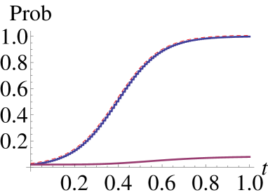
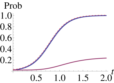
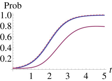
Figure 1: Quantum Jarzynski annealing for the database search problem from $N=50$ items ($N$ denotes the size of the Hilbert space). The probabilities to find the desired state are plotted for $\tau=1,2$, and $5$ from top to bottom. The dashed curves denote the instantaneous Gibbs-Boltzmann factor for reference. The upper solid curves (blue curves) representing the results by QJA are fixed to these reference curves, while the lower ones (red ones) express the time-dpendent results by the ordinary QA.

The plots by QJA (upper curves) are indistinguishable from the reference curve representing the instantaneous Gibbs-Boltzmann factor for the minimum state $i=0$. In contrast, one finds that QA (lower curves) needs sufficiently slow control of the quantum fluctuations to efficiently find the minimum.

The second example is to search the minimum from a one-dimensional random potential. We consider to find the minimum of the Hamiltonian $H_{0}=-\sum_{i=1}^{N}V_{i}|i\rangle\langle i|$, where $V_{i}$ denotes the potential energy at site $i$. We choose $\{V_{i}\}$ randomly. We again compare the case for $N=50$ sites by QJA and QA. By a linear schedule for increasing the parameter $\beta(t)$ from $0$ to $100$, we carry out QA without the exponentiated work operations and QJA. Figure 2 shows the comparison between the probability for finding the ground state by QA and QJA for different schedules $\tau=1,10$, and $100$.

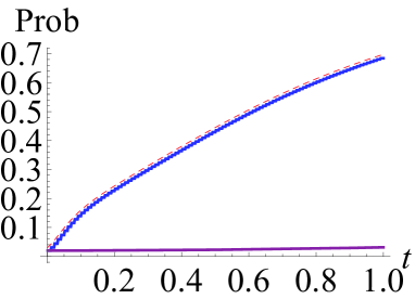
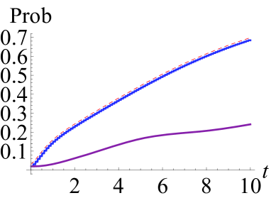
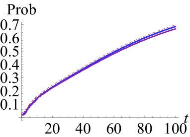
Figure 2: Quantum Jarzynski annealing for the random-potential problem for $N=50$ sites ($N$ denotes the size of the Hilbert space). The probabilities to find the minimum-potential site are plotted for $\tau=1,10$, and $100$ from top to bottom. The same symbols as in Fig. 1 are used.

On finds that the plots by QJA (upper curves) are again indistinguishable from the reference curve. QA (lower curves) needs sufficiently slow decrease of quantum fluctuations to efficiently find the site with the minimum potential.

QJA does not suffer from the energy-gap closure by increasing the system size and gives the probability to obtain the ground state independently of a predetermined schedule. Both of the above cases indeed show that the results of QJA does not depend on the computational time $\tau$.

To realize QJA in an actual quantum computation, we need to implement the exponentiated work operation $W(\sigma_{k};t_{k})$, since it looks like a non-unitary operator. We can construct this operation as a unitary operation by using an extra quantum system WQ ; Ohzeki . Instead of cut “time”, we need another resource like a “memory” in quantum computation. Fortunately, the amount of needed memory does not diverge exponentially by an increase of the system size $N$. Thus the results by QJA shown here imply that we may overcome the difficulties in hard optimization problems and solve them in a reasonable time. However, the above instances do not represent hard optimization problems as in the preceding section with an exponentially vanishing energy gap. In that sense, our results are preliminary and future work should clarify the efficiency of QJA for such hard problems.

V Summary

In this paper we first reviewed QA, which is a generic algorithm to approximately find the solution to optimization problems. The method is based on the adiabatic evolution of quantum systems. A sufficient condition to efficiently find the ground state by QA is given by the inverse square of the energy gap. The same analysis in conjunction with the classical-quantum mapping enables us to reproduce the convergence condition of SA, which is another approximate solver exploiting thermal fluctuations. Recent investigations disclosed the bottleneck of QA, the exponential closure of the energy gap. According to the prediction by the adiabatic theorem, QA does not work efficiently on problems with such a bottleneck. We thus have to invent an alternative way to efficiently find the optimal solution with the energy gap vanishing exponentially with the system size.

We next showed an application of JE to QA as one of the possible improvements of QA, using the fact that we can map a quantum system close to the instantaneous ground state to a thermal classical system in quasi-equilibrium by the classical-quantum mapping. This protocol keeps the quantum system to be the ground state expressing the instantaneous equilibrium state. The cost for the realization of QJA in quantum computation does not diverge exponentially as the system size increases, which is the essentially different point from ordinary QA. This idea has been shown to work in a few examples with a small Hilbert space. It is a future problem to test this method for problems of much larger scales and hard ones with the exponential closure of the energy gap.

- (1) T. Kadowaki, and H. Nishimori, Phys. Rev. E 58, 5355 (1998).
- (2) T. Kadowaki, Study of optimization problems by quantum annealing, PhD thesis, Tokyo Institute of Technology, (1999); e-print arXiv:0205020 [quant-ph].
- (3) A. B. Finnila, M. A. Gomez, C. Sebenik, S. Stenson, and J. D. Doll, Chem. Phys. Lett. 219, 343 (1994)
- (4) A. Das, and B. K. Charkrabarti, Quantum Annealing and Related Optimization Methods, Lecture Notes in Physics Vol.679 Springer, Berlin, (2005).
- (5) G. E. Santoro, and E. Tosatti, J. Phys. A 39, R393 (2006)
- (6) A. Das, and B. K. Chakrabarti, Rev. Mod. Phys. 80, 1061 (2008)
- (7) S. Morita, and H. Nishimori, J. Math. Phys. 49, 125210 (2008)
- (8) A. K. Hartmann, and M. Weigt, Phase Transitions in Combinatorial Optimization Problems: Basics, Algorithms and Statistical Mechanics Wiley-VCH, Weinheim, (2005).
- (9) E. Farhi, J. Goldstone, S. Gutomann, and M. Sipser, e-print arXiv:0001106 [quant-ph].
- (10) M. R. Garey, and D. S. Johnson, Computers and Intractability: A Guide to the Theory of NP-Completeness, Freeman, San Francisco, (1979).
- (11) S. Kirkpatrick, S. D. Gelett, and M. P. Vecchi, Science, 220, 671 (1983)
- (12) E. Aarts, and J. Korst, Simulated Annealing and Boltzmann Machines: A Stochastic Approach to Combinatorial Optimization and Neural Computing (Wiley, New York, 1984).
- (13) C. Jarzynski, Phys. Rev. Lett. 78, 2690 (1997)
- (14) C. Jarzynski, Phys. Rev. E 56, 5018 (1997)
- (15) R. M. Neal, Statistics and Computing, 11, 125 (2001)
- (16) Y. Iba, Trans. Jpn. Soc. Artif. Intel.16, 279 (2001)
- (17) K. Hukushima, and Y. Iba, AIP. Conf. Proc. 690, 200 (2003)
- (18) M. Ohzeki, and H. Nishimori, e-print arXiv:1003.5453 [cond-mat.dis-nn].
- (19) M. Ohzeki, and H. Nishimori, work in progress.
- (20) J. Roland, and N. J. Cerf, Phys. Rev. A 65, 042308 (2002)
- (21) S. Suzuki, and M. Okada, J. Phys. Soc. Jpn. 74,1649 (2005)
- (22) L. K. Grover, Phys. Rev. Lett. 79, 325 (1997)
- (23) S. Morita, and H. Nishimori, J. Phys. A: Math. and Gen. 39, 13903 (2006)
- (24) S. Geman and D. Geman, IEEE Trans. Pattern Anal. Mach. Intell. PAMI-6, 721 (1984)
- (25) S. Morita, and H. Nishimori, J. Phys. Soc. Jpn. 76 064002 (2007)
- (26) T. W. B. Kibble, Phys. Rep. 67, 183 (1980)
- (27) W. H. Zurek, Nature 317, 505 (1985)
- (28) W. H. Zurek, U. Dorner, and P. Zoller, Phys. Rev. Lett. 95, 105701 (2005)
- (29) J. Dziarmaga, Phys. Rev. Lett. 95, 245701 (2005)
- (30) J. Dziarmaga, Phys. Rev. B 74, 064416 (2006)
- (31) S. Suzuki, J. Stat. Mech. P03032 (2009)
- (32) G. Biroli, L. F. Cugliandolo, A. Sicilia, e-print arXiv:1001.0693v1 [cond-mat.stat-mech].
- (33) B. Derrida, Phys. Rev. Lett. 45, 79 (1980)
- (34) T. Jörg, F. Krzakala, J. Kurchan, and A. C. Maggs, Phys. Rev. Lett. 101, 147204 (2008)
- (35) A. P. Young, S. Knysh, and V. N. Smelyanskiy, Phys. Rev. Lett. 101, 170503 (2008)
- (36) A. P. Young, S. Knysh, and V. N. Smelyanskiy, Phys. Rev. Lett. 104, 020502 (2010)
- (37) T. Jörg, F. Krzakala, J. Kurchan, A. C. Maggs, and J. Pujos, Euro. Phys. Lett. 89, 40004 (2010)
- (38) R. D. Somma, C. D. Batista, and G. Ortiz, Phys. Rev. Lett. 99, 030603 (2007)
- (39) H. Orland, J. Phys. Soc. Jpn. 78, 103002 (2009)
- (40) R. C. Lua, and A. Y. Grosberg, J. Phys. Chem. B 109, 6805 (2005)
- (41) C. Jarzynski, Phys. Rev. E 73, 046105 (2006)
- (42) C. Chatelain, and D. Karevski, J. Stat. Mech. (2006) P06005.
- (43) P. Wocjan, C. Chiang, D. Nagaj, and A. Abeyesinghe, Phys. Rev. A 80, 022340 (2009)
- (44) M. Ohzeki, work in progress.