The MUSIC Algorithm for Sparse Objects: A Compressed Sensing Analysis

Abstract.

The MUSIC algorithm, and its extension for imaging sparse extended objects, with noisy data is analyzed by compressed sensing (CS) techniques. A thresholding rule is developed to augment the standard MUSIC algorithm. The notion of restricted isometry property (RIP) and an upper bound on the restricted isometry constant (RIC) are employed to establish sufficient conditions for the exact localization by MUSIC with or without noise.

In the noiseless case, the sufficient condition gives an upper bound on the numbers of random sampling and incident directions necessary for exact localization. In the noisy case, the sufficient condition assumes additionally an upper bound for the noise-to-object ratio in terms of the RIC and the dynamic range of objects. This bound points to the superresolution capability of the MUSIC algorithm. Rigorous comparison of performance between MUSIC and the CS minimization principle, Basis Pursuit Denoising (BPDN), is given.

In general, the MUSIC algorithm guarantees to recover, with high probability, $s$ scatterers with $n=\mathcal{O}(s^{2})$ random sampling and incident directions and sufficiently high frequency.

For the favorable imaging geometry where the scatterers are distributed on a transverse plane MUSIC guarantees to recover, with high probability, $s$ scatterers with a median frequency and $n=\mathcal{O}(s)$ random sampling/incident directions.

Moreover, for the problems of spectral estimation and source localizations both BPDN and MUSIC guarantee, with high probability, to identify exactly the frequencies of random signals with the number $n=\mathcal{O}(s)$ of sampling times. However, in the absence of abundant realizations of signals, BPDN is the preferred method for spectral estimation. Indeed, BPDN can identify the frequencies approximately with just one realization of signals with the recovery error at worst linearly proportional to the noise level.

Numerical results confirm that BPDN outperforms MUSIC in the well-resolved case while the opposite is true for the under-resolved case, giving abundant evidences for the superresolution capability of the MUSIC algorithm.

Another advantage of MUSIC over BPDN is the former’s flexibility with grid spacing and guarantee of approximate localization of sufficiently separated objects in an arbitrarily refined grid. The localization error is bounded from above by $\mathcal{O}(\lambda s)$ for general configurations and by $\mathcal{O}(\lambda)$ for objects distributed in a transverse plane.

1. Introduction

The MUSIC (standing for MUltiple-Signal-Classification) algorithm is a well-known method in signal processing for estimating the individual frequencies of multiple time-harmonic signals [5, 21]. Mathematically, MUSIC is essentially a method of characterizing the range of the covariance matrix of the signals (see Section 6 for details).

MUSIC was originally developed to estimate the direction of arrival for source localization [19]. Later, the MUSIC algorithm is extended to imaging of point scatterers [6]. A proof of a sufficient condition for the exact recovery of the object support in the noiseless case is given in [16] (see also [15]) which is reproduced in Proposition 1 below. The performance guarantee is general but qualitative in nature. Neither does it take into account the effect of noise which is important for assessing the superresolution effect.

The main purpose of this paper is to give a quantitative performance evaluation for the MUSIC algorithm in terms of how many data are needed and how they may be collected in order to exactly recover the locations of given (large) number of objects, be they sources, scatterers or frequencies as well as how much noise the MUSIC algorithm can tolerate. Our approach is based on recent advances in compressed sensing theory ([1, 2, 18] and references therein) and applications to imaging ([9, 10, 11] and references therein).

A main result for localizing scatterers obtained in the present paper has the following flavor (more details later): Let $\xi_{\rm max}$ and $\xi_{\rm min}$ be, respectively, the strengths of the strongest and weakest (nonzero) scatterers, $\delta^{\pm}_{s}$ the (generalized) restricted isometry constants (RIC) of order $s$ and $\varepsilon$ the level of noise in the data. If the noise-to-scatterer ratio (NSR) obeys the upper bound

(1) $${\varepsilon\over\xi_{\rm min}}<\sqrt{{(1+\delta^{+}_{s})^{2}}{\xi^{2}_{\rm max}\over\xi^{2}_{\rm min}}+(1-\delta^{-}_{s})^{2}\Delta}-{(1+\delta^{+}_{s})}{\xi_{\rm max}\over\xi_{\rm min}}$$

where

$$\Delta = {1\over 2}-{1\over 2}{1\over\sqrt{\sqrt{2}\Gamma_{\mathcal{S}}+1}}$$

and $\Gamma_{\mathcal{S}}$ (defined in (19)) is a measure of the independence of the column vectors outside the object support from the range of the data matrix then the MUSIC imaging function $J^{\varepsilon}$ with the thresholding rule

(2) $$\left\{\mathbf{r}\in{\mathcal{K}}:J^{\varepsilon}(\mathbf{r})\geq 2\left(1-{\delta^{-}_{s+1}(1+\delta^{+}_{s})\over 2+\delta_{s}^{+}-\delta^{-}_{s+1}}\right)^{-2}\right\}$$

recovers exactly the locations of the $s$ scatterers (cf. Theorem 2, Section 3). Compressed sensing theory comes into play in addressing the dependence of RIC on the frequency, the number and distribution of random sampling directions (or sensors), the number of scatterers and the inter-scatterer distances.

In the super-resolution regime, the $\delta_{s}^{-}$ tends to $1$ and $\Gamma_{\mathcal{S}}$ tends to zero, rendering the right hand side of (1) approximately

(3) $${(1-\delta_{s}^{-})^{2}\Delta\over 2(1+\delta_{s}^{+})\xi_{\rm max}/\xi_{\rm min}}$$

where $\xi_{\rm max}/\xi_{\rm min}$ is the dynamic range of the scatterers. For a NSR smaller than (3) the $s$ scatterers can still be perfectly localized by the MUSIC algorithm with the thresholding rule (2) where the threshold is approximately

$${2\over(1-\delta_{s+1}^{-})^{2}}\left({1+\delta_{s}^{+}\over 2+\delta_{s}^{+}}\right)^{2}\gg 1.$$

Previous observation [17] and our numerical results (Section 8) lend support to this superresolution effect of the MUSIC algorithm.

First let us review the inverse scattering problem and the MUSIC imaging method.

1.1. Inverse scattering

Consider the scattering of the incident plane wave

(4) $$u^{\rm i}(\mathbf{r})=e^{i\omega\mathbf{r}\cdot\hat{\mathbf{d}}}$$

by the variable refractive index $n^{2}(\mathbf{r})=1+\xi(\mathbf{r})$ where $\hat{\mathbf{d}}$ is the incident direction. The scattered field satisfies the Lippmann-Schwinger equation

(5) $$u^{\rm s}(\mathbf{r}) = \omega^{2}\int_{\mathbb{R}^{d}}\xi(\mathbf{r}^{\prime})\left(u^{\rm i}(\mathbf{r}^{\prime})+u^{\rm s}(\mathbf{r}^{\prime})\right)G(\mathbf{r},\mathbf{r}^{\prime})d\mathbf{r}^{\prime},\quad d=2,3$$

where $G(\mathbf{r},\mathbf{r}^{\prime})$ is the Green function of the operator $-(\Delta+\omega^{2})$ [16]. We assume that the wave speed is unity and hence the frequency equals the wavenumber $\omega$.

The scattered field has the far-field asymptotic

(6) $$u^{\rm s}(\mathbf{r})={e^{i\omega|\mathbf{r}|}\over|\mathbf{r}|^{(d-1)/2}}\left(A(\hat{\mathbf{r}},\hat{\mathbf{d}})+\mathcal{O}(|\mathbf{r}|^{-1})\right),\quad\hat{\mathbf{r}}=\mathbf{r}/|\mathbf{r}|,$$

where the scattering amplitude $A$ is determined by the formula

(7) $$A(\hat{\mathbf{r}},\hat{\mathbf{d}}) = {\omega^{2}\over 4\pi}\int_{\mathbb{R}^{d}}d\mathbf{r}^{\prime}\xi(\mathbf{r}^{\prime})u(\mathbf{r}^{\prime})e^{-i\omega\mathbf{r}^{\prime}\cdot\hat{\mathbf{r}}}.$$

In the Born regime, the total field $u$ on the right hand side of (7) can be replaced by the incident field $u^{\rm i}$.

The main objective of inverse scattering then is to reconstruct the medium inhomogeneities $\xi$ from the knowledge about the scattering amplitude $A(\hat{\mathbf{r}},\hat{\mathbf{d}})$.

Figure 1. Far-field imaging geometry

Next we recall the MUSIC algorithm as applied to localization of point scatterers.

1.2. MUSIC for point scatterers

Let ${\mathcal{S}}=\left\{\mathbf{r}_{j}:j=1,...,s\right\}$ be the locations of the scatterers. Let $\xi_{j}\neq 0,j=1,...,s$ be the strength of the scatterers. We will make the Born approximation first and discuss how to lift this restriction at the end of the section (Remark 2). For the discrete medium the scattering amplitude becomes the finite sum

(8) $$A(\hat{\mathbf{r}},\hat{\mathbf{d}}) = {\omega^{2}\over 4\pi}\sum_{j=1}^{s}\xi_{j}u^{\rm i}(\mathbf{r}_{j})e^{-i\omega\mathbf{r}_{j}\cdot\hat{\mathbf{r}}_{j}}$$

under the Born approximation.

Let $\hat{\mathbf{d}}_{l},l=1,...,m$ and $\hat{\mathbf{s}}_{k},k=1,...,n$ be, respectively, the incident and sampling directions. For each incident field $\hat{\mathbf{d}}_{l},l=1,...,m,$ the scattering amplitude is measured in all $n$ directions $\hat{\mathbf{s}}_{k},k=1,...,n$. The whole measurement data consist of the scattering amplitudes for all pairs of $(\hat{\mathbf{d}}_{l},\hat{\mathbf{s}}_{k})$.

Define the data matrix $\mathbf{Y}=(Y_{k,l})\in\mathbb{C}^{n\times m}$ as

(9) $$Y_{k,l}\sim A(\hat{\mathbf{s}}_{k},\hat{\mathbf{d}}_{l}),\quad k=1,...,n,\quad l=1,...,m$$

where we keep open the option of normalizing $\mathbf{Y}$ in order to simplify the set-up. The data matrix is related to the object matrix

$$\mathbf{X}=\hbox{\rm diag}(\xi_{j})\in\mathbb{C}^{s\times s},\quad j=1,...s$$

by the measurement matrices $\mathbf{\Phi}$ and ${\mathbf{\Psi}}$ as

(10) $$\mathbf{Y}=\mathbf{\Phi}\mathbf{X}{\mathbf{\Psi}}^{*}$$

where $\mathbf{\Phi}$ and ${\mathbf{\Psi}}$ are, respectively,

(11) $$\Phi_{k,j} = {1\over\sqrt{n}}e^{-i\omega\hat{\mathbf{s}}_{k}\cdot\mathbf{r}_{j}}\in\mathbb{C}^{n\times s}$$

(12) $$\Psi_{l,j} = {1\over\sqrt{n}}e^{-i\omega\hat{\mathbf{d}}_{l}\cdot\mathbf{r}_{j}}\in\mathbb{C}^{m\times s}$$

after proper normalization. Both (11) and (12) are normalized to have columns of unit 2-norm. We extend the formulation (10)-(12) to the case of sparse extended objects in Appendix A.

Note that both $\mathbf{\Phi}$ and ${\mathbf{\Psi}}$ are unknown and (10) can be inverted only after the locations of scatterers are determined. This is what the MUSIC algorithm is designed to accomplish.

The standard version of MUSIC algorithm deals with the case of $n=m$ and $\hat{\mathbf{s}}_{k}=\hat{\mathbf{d}}_{k},k=1,...,n$ as stated in the following result.

Proposition 1.

[15, 16] Let $\{\hat{\mathbf{s}}_{k}=\hat{\mathbf{d}}_{k},k\in\mathbb{N}\}$ be a countable set of directions such that any analytic function on the unit sphere that vanishes in $\hat{\mathbf{s}}_{k},\forall k\in\mathbb{N}$ vanishes identically. Let ${\mathcal{K}}\subset\mathbb{R}^{3}$ be a compact subset containing ${\mathcal{S}}$. Then there exists $n_{0}$ such that for any $n\geq n_{0}$ the following characterization holds for every $\mathbf{r}\in{\mathcal{K}}$:

(13) $$\mathbf{r}\in{\mathcal{S}}\,\,\hbox{ if and only if }\,\,\phi_{\mathbf{r}}\equiv{1\over\sqrt{n}}(e^{-i\omega\hat{\mathbf{s}}_{1}\cdot\mathbf{r}},e^{-i\omega\hat{\mathbf{s}}_{2}\cdot\mathbf{r}},\cdots,e^{-i\omega\hat{\mathbf{s}}_{n}\cdot\mathbf{r}})^{T}\in\hbox{\rm Ran}(\mathbf{\Phi}).$$

Moreover, the ranges of $\mathbf{\Phi}$ and $\mathbf{Y}$ coincide.

Remark 1.

As a consequence, $\mathbf{r}\in{\mathcal{S}}$ if and only if ${\mathcal{P}}\phi_{\mathbf{r}}=0$ where ${\mathcal{P}}$ is the orthogonal projection onto the null space of $\mathbf{Y}^{*}$ (Fredholm alternative). And the locations of the scatterers can be identified by the singularities of the imaging function

(14) $$J(\mathbf{r})={1\over|{\mathcal{P}}\phi_{\mathbf{r}}|^{2}}$$

[5].

Moreover, once the locations are exactly recovered, then both $\mathbf{\Phi}$ and ${\mathbf{\Psi}}$ are known explicitly and the strength $\xi_{j},j=1,...,s$ of scatterers can be determined by inverting the linear equation (10) which is an over-determined system.

Remark 2.

The assumptions of Proposition 1 can be relaxed: instead of $\hat{\mathbf{s}}_{k}=\hat{\mathbf{d}}_{k},\forall k$, it suffices to have ${\mathbf{\Psi}}\in\mathbb{C}^{m\times s}$ which has rank $s$.

In light of this observation, it is also straightforward to extend the performance guarantee for the Born scattering case to the multiple-scattering case. In the latter case, ${\mathbf{\Psi}}$ consists of entries which are the total field evaluated at $\mathbf{r}_{j}$ for the incident direction $\hat{\mathbf{d}}_{l}$, i.e.

(15) $$\Psi_{l,j}=u^{*}(\mathbf{r}_{j};\hat{\mathbf{d}}_{l}).$$

What is really needed is that ${\mathbf{\Psi}}\in\mathbb{C}^{m\times s}$ has rank $s$ since then $\mathbf{Z}=\mathbf{X}{\mathbf{\Psi}}^{*}$ and $\mathbf{X}$ share the same support (see more on this in Section 2). Generically this is true for sufficiently large $m$ as we will show below.

Define the incident and full field vectors at the locations of the scatterers:

$$U^{\rm i}(\hat{\mathbf{d}}_{l}) = (u^{\rm i}(\mathbf{r}_{1};\hat{\mathbf{d}}_{l}),...,u^{\rm i}(\mathbf{r}_{s};\hat{\mathbf{d}}_{l}))^{T}\in\mathbb{C}^{s}$$

$$U(\hat{\mathbf{d}}_{l}) = (u(\mathbf{r}_{1};\hat{\mathbf{d}}_{l}),...,u(\mathbf{r}_{s}:\hat{\mathbf{d}}_{l}))^{T}\in\mathbb{C}^{s}.$$

Denote

(16) $${\mathbf{G}}=[(1-\delta_{ij})G(\mathbf{r}_{j},\mathbf{r}_{i})]\in\mathbb{C}^{s\times s}.$$

The discrete version of the Lippmann-Schwinger equation (i.e. the Foldy-Lax equation) can be written as

(17) $$U(\hat{\mathbf{d}}_{l})=U^{\rm i}(\hat{\mathbf{d}}_{l})+\omega^{2}{\mathbf{G}}\mathbf{X}U(\hat{\mathbf{d}}_{l}),\quad l=1,...,m.$$

The $\delta_{ij}$ terms in (16) represent the singular self-energy terms of point scatterers and should be removed for self consistency.

Denote ${\mathbf{U}}^{\rm i}=[U^{\rm i}(\hat{\mathbf{d}}_{1}),...,U^{\rm i}(\hat{\mathbf{d}}_{m})]\in\mathbb{C}^{s\times m}$ and ${\mathbf{U}}=[U(\hat{\mathbf{d}}_{1}),...,U(\hat{\mathbf{d}}_{m})]\in\mathbb{C}^{s\times m}$. Suppose that $\omega^{-2}$ is not an eigenvalue of ${\mathbf{G}}\mathbf{X}$. Then we can invert eq. (17) to obtain

$${\mathbf{U}}=(\mathbf{I}-\omega^{2}{\mathbf{G}}\mathbf{X})^{-1}{\mathbf{U}}^{\rm i}.$$

Hence ${\mathbf{U}}$ has rank $s$ if ${\mathbf{U}}^{\rm i}$ does. Indeed, for sufficiently high frequency $\omega$ and $m$ randomly selected incident directions with sufficiently large ratio $\sqrt{m}/s$, ${\mathbf{U}}^{\rm i}$ has rank $s$ with high probability (Propositions 3 and 4 below).

For some special imaging geometry it is possible to reduce the number of incident and sampling directions to $\mathcal{O}(s)$ (Section 4).

1.3. Outline

Proposition 1 says that if the number of sampling directions is sufficiently large then the locations of the $s$ scatterers can be identified by the $s$ singularities of $J$. However, the condition is only qualitative in the sense that an estimate for the threshold $n_{0}$ is not given. It would be of obvious interest to know, e.g. how $n_{0}$ scales with $s$ when $s$ is large and when the conventional wisdom ($n_{0}=s+1$) derived from counting dimensions is true. Also, how much noise can the MUSIC algorithm tolerate?

However, unless additional constraints are imposed on the measurement scheme (the frequency, the incident and sampling directions etc), it is unlikely to make progress toward obtaining an useful estimate which is the objective of the present study. In [6] a geometric constraint on the configuration of sensors and objects has been pointed out for exact recovery in the absence of noise. Moreover, it seems possible that a non-vanishing portion of $s$ randomly distributed scatterers may not be exactly recovered in the presence of machine error no matter how large $n$ is (Figure 5, middle panel, and Figure 7, right panel).

Let us briefly sketch our approach and results:We shall discretize the problem by using a finite grid for the computation domain ${\mathcal{K}}$ and put the problem in a probabilistic setting by using random sampling directions. Moreover, we consider noisy data and aim for a result for stable recovery by MUSIC. For the case of well-resolved grids, we show by using the compressed sensing techniques that for the NSR obeying (1) and with high probability, $n_{0}=\mathcal{O}(s^{2})$ for general configuration of $s$ objects and $n_{0}=\mathcal{O}(s)$ for objects distributed on a transverse plane. For the case of under-resolved grids, we seek sufficient conditions for approximate, instead of exact, localization of objects and we show that for sufficiently small NSR and with high probability, the localization error is $\mathcal{O}(\lambda s)$ with $n=\mathcal{O}(s^{2})$ for a general object configuration and the localization error is $\mathcal{O}(\lambda)$ with $n=\mathcal{O}(s)$ for objects distributed in a transverse plane.

Our plan for the rest of the paper is to first give a sensitivity analysis for MUSIC and derive the condition for exact recovery with noisy data under which the MUSIC algorithm based on the perturbed data matrix can still recover exactly the object support (Section 2). Next, we review the basic notion of compressed sensing (CS) theory and show how it naturally lends itself to a proof of exact localization by MUSIC (Section 3). We show that with generic, random sampling and sufficiently high frequency the MUSIC algorithm can, with high probability, recover $s$ scatterers with $n=\mathcal{O}(s^{2})$ sampling and incident directions (Corollary 2). Then we consider a favorable imaging geometry where the scatterers are distributed on a transverse plane (Section 4). We show that with median frequency the MUSIC algorithm can recover, with high probability, $s$ scatterers with $n=\mathcal{O}(s)$ sampling and incident directions (Corollary 3). Next we analyze the performance guarantee of the compressed sensing principle, Basis Pursuit Denoising (BPDN) (Section 5) and show that in the generic situation BPDN with sufficiently high frequency can recover $s$ scatterers with $n=\mathcal{O}(s^{2})$ sampling directions and just one incident wave (Remark 10) while for the favorable geometry of planar objects BPDN can recover $s$ scatterers with $n=\mathcal{O}(s)$ sampling directions and one incident wave (Remark 9). In Section 6 we return to the original applications of MUSIC and perform the compressed sensing analysis of the performance of MUSIC as applied to spectral estimation and source localization. We show that the MUSIC algorithm can, with high probability, identify exactly the frequencies of random signals with the number $n=\mathcal{O}(s)$ of sampling times (Corollary 6 and Remark 11). We discuss MUSIC in the setting with an arbitrarily fine grid and give error bounds in Section 7. Numerical tests are given in Section 8 where the superresolution capability of MUSIC and the noise sensitivity are studied. We conclude in Section 9. We give an extension of the MUSIC algorithm to the case of extended objects in Appendix A and a proof of performance guarantee for BPDN in Appendix B.

2. Sensitivity analysis

For quantitative performance analysis of the MUSIC algorithm, we will work with the discrete setting and assume that ${\mathcal{K}}$ is a discrete set of $N$, typically large, number of points, i.e. the computation grid. The discrete setting appears naturally in applying MUSIC to imaging of extended scatterers (see Appendix A). Moreover, we consider the extension $\tilde{\mathbf{\Phi}}$ of $\mathbf{\Phi}$ which includes not only the columns $\phi_{\mathbf{r}_{j}},j=1,...,s$ representing the locations of the objects but also the columns representing all the points in ${\mathcal{K}}$. Hence $\tilde{\mathbf{\Phi}}\in\mathbb{C}^{n\times N}$ and as usual $\tilde{\mathbf{\Phi}}$ is normalized so that the columns have unit 2-norm. The ordering of the columns of $\tilde{\mathbf{\Phi}}$ is not important for our purpose as long as they correspond to the points in ${\mathcal{K}}$ in a well-defined manner. $\tilde{\mathbf{\Psi}}\in\mathbb{C}^{n\times N}$ is similarly defined. Also the extension $\tilde{\mathbf{X}}\in\mathbb{C}^{N\times N}$ of $X$ is defined by filling in zeros in all the entries outside the object support.

In terms of these notations, we can write

(18) $$\mathbf{Y}=\tilde{\mathbf{\Phi}}\tilde{\mathbf{X}}\tilde{\mathbf{\Psi}}^{*}=\sum_{j=1}^{N}\tilde{\Phi}_{j}\otimes\tilde{\Psi}_{j}^{*}\xi_{j}.$$

By a slight abuse of notation, we shall use ${\mathcal{S}}$ to denote the locations of objects in the physical domain as well as the corresponding index set. Likewise ${\mathcal{S}}^{c}$ denotes the complement set of ${\mathcal{S}}$ in the computation grid ${\mathcal{K}}$ as well as the total index set $\{1,...,N\}$. In the same vein, $\tilde{\mathbf{\Phi}}_{\mathcal{S}}$ denotes the column submatrix of $\mathbf{\Phi}$ restricted to the index set ${\mathcal{S}}$. Hence $\tilde{\mathbf{\Phi}}_{\mathcal{S}}=\mathbf{\Phi}$ and $\tilde{\mathbf{\Psi}}_{\mathcal{S}}={\mathbf{\Psi}}$.

First, let us reformulate the condition (13) for exact recovery as follows.

Note that

$$\mathbf{\Phi}\mathbf{\Phi}^{\dagger}\phi_{\mathbf{r}}$$

is the orthogonal projection of $\phi_{\mathbf{r}}$ onto the range of $\mathbf{\Phi}$ where $\mathbf{\Phi}^{\dagger}$ is the pseudo-inverse of $\mathbf{\Phi}$. Hence

$${\mathcal{P}}\phi_{\mathbf{r}}=(\mathbf{I}-\mathbf{\Phi}\mathbf{\Phi}^{\dagger})\phi_{\mathbf{r}}.$$

If $\phi_{\mathbf{r}}$ for $\mathbf{r}\in{\mathcal{S}}^{c}$ is independent of the columns of $\mathbf{\Phi}$, then

$$\phi_{\mathbf{r}}^{*}\mathbf{\Phi}\mathbf{\Phi}^{\dagger}\phi_{\mathbf{r}}<\|\phi_{\mathbf{r}}\|^{2}$$

and vice versa. Therefore (13) is equivalent to

(19) $$\Gamma_{\mathcal{S}}\equiv\min_{\mathbf{r}\in{\mathcal{S}}^{c}}\|\phi_{\mathbf{r}}\|_{2}^{-1}\|{\mathcal{P}}\phi_{\mathbf{r}}\|_{2}=\sqrt{1-\max_{\mathbf{r}\in{\mathcal{S}}^{c}}\|\phi_{\mathbf{r}}\|^{-2}\phi_{\mathbf{r}}^{*}\mathbf{\Phi}\mathbf{\Phi}^{\dagger}\phi_{\mathbf{r}}}>0.$$

The number $\Gamma_{\mathcal{S}}$ gives a measure of how “independent” $\phi_{z}$ is from the range of $\mathbf{\Phi}$ uniformly in $\mathbf{r}\in{\mathcal{S}}^{c}$.

Now we give a sensitivity analysis for MUSIC with respect to perturbation in the data matrix $\mathbf{Y}$ in terms of $\Gamma_{\mathcal{S}}$ and other parameters. We want to show what else is needed, in addition to (13), to guarantee exact recovery of the support of scatterers when the data matrix is perturbed.

The general data matrix considered in this paper has the form $\mathbf{Y}^{\varepsilon}=\mathbf{Y}+\mathbf{E}$ where $\mathbf{Y}=\mathbf{\Phi}\mathbf{X}{\mathbf{\Psi}}^{*}\in\mathbb{C}^{n\times m},m\geq s$, the number of objects. Set $\mathbf{Z}=\mathbf{X}{\mathbf{\Psi}}^{*}\in\mathbb{C}^{s\times m}$ such that $\mathbf{Y}=\mathbf{\Phi}\mathbf{Z}$ where $\mathbf{Z}$ is assumed to have rank $s$.

We shall treat $\mathbf{Z}$ as the new object matrix and consider perturbed data matrices of the form

(20) $$\mathbf{Y}^{\varepsilon}=\mathbf{\Phi}\mathbf{Z}+\mathbf{E}.$$

Note that the locations of objects represented by $\mathbf{Z}$ are identical to those represented by $\mathbf{X}=\hbox{\rm diag}(\xi_{j})$.

Set

$${\mathcal{Y}}^{\varepsilon}=\mathbf{Y}^{\varepsilon}\mathbf{Y}^{\varepsilon*}={\mathcal{Y}}+{\mathcal{E}}$$

where

(21) $${\mathcal{Y}} = \mathbf{\Phi}\mathbf{Z}\mathbf{Z}^{*}\mathbf{\Phi}^{*}\in\mathbb{C}^{n\times n}$$

(22) $${\mathcal{E}} = \mathbf{E}\mathbf{Z}^{*}\mathbf{\Phi}^{*}+\mathbf{\Phi}\mathbf{Z}\mathbf{E}^{*}+\mathbf{E}\mathbf{E}^{*}\in\mathbb{C}^{n\times n}$$

are both self-adjoint. Note that the range of ${\mathcal{Y}}$ is the same as the range of $\mathbf{\Phi}$ and under the assumption of (13) equals to the span of $\{\phi_{\mathbf{r}}:\mathbf{r}\in{\mathcal{S}}\}$.

Let $\{\mathbf{v}_{j}:j=1,...,s\}$ and $\{\mathbf{v}_{j}:j=s+1,...,n\}$, respectively, be the set of orthonormal bases for the range and null space of ${\mathcal{Y}}$. Let $\mathbf{Q}_{1}\in\mathbb{C}^{n\times s}$ and $\mathbf{Q}_{2}\in\mathbb{C}^{n\times(n-s)}$, respectively, be the matrices whose columns are exactly $\{\mathbf{v}_{j}:j=1,...,s\}$ and $\{\mathbf{v}_{j}:j=s+1,...,n\}$. Let $\mathbf{Q}=[\mathbf{Q}_{1},\mathbf{Q}_{2}]\in\mathbb{C}^{n\times n}$.

Let $\sigma_{1}\geq\sigma_{2}\geq\cdots\geq\sigma_{n}$ be the singular values of ${\mathcal{Y}}$. Denote the smallest nonzero singular value of ${\mathcal{Y}}$ by $\sigma_{\rm min}$ and set $\sigma_{\rm max}=\sigma_{1}$. If $\mathbf{Y}$ has rank $s$, then $\sigma_{\rm min}=\sigma_{s}$. We partition $\mathbf{Q}^{*}{\mathcal{E}}\mathbf{Q}$ as follows:

(23) $$\mathbf{Q}^{*}{\mathcal{E}}\mathbf{Q}=\left[\begin{matrix}{\mathcal{E}}_{11}&{\mathcal{E}}_{12}\\ {\mathcal{E}}_{21}&{\mathcal{E}}_{22}\end{matrix}\right]$$

where ${\mathcal{E}}_{11}\in\mathbb{C}^{s\times s},{\mathcal{E}}_{12}\in\mathbb{C}^{s\times(n-s)},{\mathcal{E}}_{21}\in\mathbb{C}^{(n-s)\times s},{\mathcal{E}}_{22}\in\mathbb{C}^{(n-s)\times(n-s)}$.

The following is a slight recasting of a general result of matrix perturbation theory [20].

Proposition 2.

(Theorem 2.7, Chap. V, [20]) If

(24) $${\sqrt{\|{\mathcal{E}}_{12}\|_{2}\|{\mathcal{E}}_{21}\|_{2}}\over\sigma_{\rm min}-\|{\mathcal{E}}_{11}\|_{2}-\|{\mathcal{E}}_{22}\|_{2}}<{1\over 2}$$

then there exist ${\mathbf{F}}\in\mathbb{C}^{(n-s)\times s}$ with

(25) $$\|{\mathbf{F}}\|_{2} \leq {2\|{\mathcal{E}}_{21}\|_{2}\over\sigma_{\rm min}-\|{\mathcal{E}}_{11}\|_{2}-\|{\mathcal{E}}_{22}\|_{2}}$$

such that the columns of

(26) $$\mathbf{Q}^{\varepsilon}_{1} = (\mathbf{Q}_{1}+\mathbf{Q}_{2}{\mathbf{F}})(\mathbf{I}+{\mathbf{F}}^{*}{\mathbf{F}})^{-1/2}$$

(27) $$\mathbf{Q}^{\varepsilon}_{2} = (\mathbf{Q}_{2}-\mathbf{Q}_{1}{\mathbf{F}}^{*})(\mathbf{I}+{\mathbf{F}}{\mathbf{F}}^{*})^{-1/2}$$

are, respectively, orthornormal bases for invariant subspaces of ${\mathcal{Y}}^{\varepsilon}$.

The representation of ${\mathcal{Y}}^{\varepsilon}$ with respect to $\mathbf{Q}^{\varepsilon}_{1},\mathbf{Q}^{\varepsilon}_{2}$ is, respectively,

(28) $$\Sigma^{\varepsilon}_{1} = (\mathbf{I}+{\mathbf{F}}^{*}{\mathbf{F}})^{1/2}\left[\Sigma_{1}+{\mathcal{E}}_{11}+{\mathcal{E}}_{12}{\mathbf{F}}\right](\mathbf{I}+{\mathbf{F}}^{*}{\mathbf{F}})^{-1/2}$$

(29) $$\Sigma_{2}^{\varepsilon} = (\mathbf{I}+{\mathbf{F}}{\mathbf{F}}^{*})^{-1/2}\left[{\mathcal{E}}_{22}-{\mathbf{F}}{\mathcal{E}}_{12}\right](\mathbf{I}+{\mathbf{F}}{\mathbf{F}}^{*})^{1/2}$$

where $\Sigma_{1}=\hbox{diag}(\sigma_{1},\sigma_{2},...,\sigma_{\rm min})$.

Corollary 1.

Let $\rho_{*}\in(1/5,1/4)$ be the only real root of the cubic polynomial $p(\rho)=1-8\rho+20\rho^{2}-20\rho^{3}$ and suppose

(30) $${\|{\mathcal{E}}\|_{2}\over\sigma_{\rm min}}<\rho_{*}.$$

Then $\hbox{\rm Ran}(\mathbf{Q}^{\varepsilon}_{1})$ is the singular subspace associated with the $s$ largest singular values of $\mathbf{Y}^{\varepsilon}$ and $\hbox{\rm Ran}(\mathbf{Q}^{\varepsilon}_{2})$ the singular subspace associated with the rest of the singular values.

Proof.

It suffices to show that under (30) the smallest singular value of $\Sigma_{1}$ is larger than the largest singular value of $\Sigma_{2}$.

Since $\rho_{*}<1/4$, condition (30) implies that

$${\|{\mathcal{E}}\|_{2}\over\sigma_{\rm min}-2\|{\mathcal{E}}\|_{2}}<{1\over 2}$$

which in turn implies (24). Note that under this condition $\|{\mathbf{F}}\|_{2}\leq 1$. By Proposition 2 we have

$$\|\Sigma^{\varepsilon}_{2}\|_{2} \leq \|\mathbf{I}+{\mathbf{F}}{\mathbf{F}}^{*}\|^{1/2}_{2}\|{\mathcal{E}}_{22}-{\mathbf{F}}{\mathcal{E}}_{12}\|_{2}$$

$$\leq \left(1+{4\|{\mathcal{E}}\|_{2}^{2}\over(\sigma_{\rm min}-2\|{\mathcal{E}}\|_{2})^{2}}\right)^{1/2}\left(\|{\mathcal{E}}\|_{2}+{2\|{\mathcal{E}}\|_{2}^{2}\over\sigma_{\rm min}-2\|{\mathcal{E}}\|_{2}}\right)$$

On the other hand,

$$\min_{\|{\mathbf{e}}\|_{2}=1}\|\Sigma^{\varepsilon}_{1}{\mathbf{e}}\|_{2} = \min_{\|{\mathbf{e}}\|_{2}=1}\|(\Sigma_{1}+{\mathcal{E}}_{11}+{\mathcal{E}}_{12}{\mathbf{F}}){\mathbf{e}}\|\|\mathbf{I}+{\mathbf{F}}^{*}{\mathbf{F}}\|^{-1/2}_{2}$$

$$\geq \left(\sigma_{\rm min}-\|{\mathcal{E}}\|_{2}-{2\|{\mathcal{E}}\|^{2}_{2}\over\sigma_{\rm min}-2\|{\mathcal{E}}\|_{2}}\right)\left(1+{4\|{\mathcal{E}}\|_{2}^{2}\over(\sigma_{\rm min}-2\|{\mathcal{E}}\|_{2})^{2}}\right)^{-1/2}.$$

Let

$$\rho={\|{\mathcal{E}}\|_{2}\over\sigma_{\rm min}}.$$

Imposing that the right hand side of (2) is greater than that of (2) leads to the inequality

$$p(\rho) = (1-2\rho)^{3}-2\rho(1-2\rho)^{2}-4\rho^{3}$$

$$= 1-8\rho+20\rho^{2}-20\rho^{3}>0$$

which holds for $\rho<\rho_{*}$, the only real root of $p(x)$. It is readily verified that $\rho_{*}\in(1/5,1/4).$

∎

In view of Corollary 1, it is natural to call $\hbox{\rm Ran}(\mathbf{Q}^{\varepsilon}_{2})$ the noise subspace and $\hbox{\rm Ran}(\mathbf{Q}_{1}^{\varepsilon})$ the signal (or object) subspace.

Let ${\mathcal{P}}^{\varepsilon}$ be the orthogonal projection onto the noise subspace and define the MUSIC imaging function for the noisy data

$$J^{\varepsilon}(\mathbf{r})={1\over|{\mathcal{P}}^{\varepsilon}\phi_{\mathbf{r}}|^{2}}.$$

We are ready to state the first main result of the paper.

Theorem 1.

Let ${\mathcal{Y}}^{\varepsilon}={\mathcal{Y}}+{\mathcal{E}}$ where ${\mathcal{Y}}$ and ${\mathcal{E}}$ are given by (21)-(22).

Suppose $\phi_{\mathbf{r}}\in{\rm Ran}(\mathbf{\Phi})$ if and only if $\mathbf{r}\in{\mathcal{S}}$. Then the condition

(33) $${\|{\mathcal{E}}\|_{2}\over\sigma_{\rm min}} < \Delta={1\over 2}-{1\over 2}{1\over\sqrt{\sqrt{2}\Gamma_{\mathcal{S}}+1}}$$

implies that the $s$ highest peaks of $J^{\varepsilon}(\mathbf{r})$ coincide with the true locations of objects. Indeed, the object locations can be identified by the thresholding rule:

(34) $$\left\{\mathbf{r}\in{\mathcal{K}}:J^{\varepsilon}(\mathbf{r})\geq 2\Gamma_{\mathcal{S}}^{-2}\right\}.$$

Proof.

Let $\{\mathbf{v}_{j}+\delta\mathbf{v}_{j}:j=s+1,...,n\}$ be the columns of $\mathbf{Q}^{\varepsilon}_{2}$. Clearly, $\delta\mathbf{v}_{j}$ is the $(j-s)$-th column of $\mathbf{Q}^{\varepsilon}_{2}-\mathbf{Q}_{2}$. Now we have

$$\|\mathbf{Q}^{\varepsilon}_{2}-\mathbf{Q}_{2}\|_{2} \leq \|\mathbf{Q}_{1}{\mathbf{F}}^{*}(\mathbf{I}+{\mathbf{F}}{\mathbf{F}}^{*})^{-1/2}\|_{2}+\|\mathbf{Q}_{2}(\mathbf{I}+{\mathbf{F}}{\mathbf{F}}^{*})^{-1/2}-\mathbf{Q}_{2}\|_{2}$$

$$\leq \|\mathbf{Q}_{1}{\mathbf{F}}^{*}\|_{2}+\|(\mathbf{I}+{\mathbf{F}}{\mathbf{F}}^{*})^{-1/2}-\mathbf{I}\|_{2}$$

whose first term is bounded by $\|{\mathbf{F}}\|_{2}$ and whose second term is bounded by

$$\|(\mathbf{I}+{\mathbf{F}}{\mathbf{F}}^{*})^{-1/2}-\mathbf{I}\|_{2} = \|(\mathbf{I}+{\mathbf{F}}{\mathbf{F}}^{*})^{-1/2}(\mathbf{I}+(\mathbf{I}+{\mathbf{F}}{\mathbf{F}}^{*})^{1/2})^{-1}{\mathbf{F}}{\mathbf{F}}^{*}\|_{2}$$

$$\leq {1\over 2}\|{\mathbf{F}}\|_{2}^{2}.$$

Hence

(35) $$\|\delta\mathbf{v}_{j}\|_{2} \leq \|\mathbf{Q}^{\varepsilon}_{2}-\mathbf{Q}_{2}\|_{2}\leq\|{\mathbf{F}}\|_{2}+{1\over 2}\|{\mathbf{F}}\|_{2}^{2}\leq{2\rho(1-\rho)\over(1-2\rho)^{2}},\quad j=s+1,...,n,$$

where $\rho=\|{\mathcal{E}}\|_{2}/\sigma_{\rm min}$.

By Corollary 1 $\{\mathbf{v}_{j}+\delta\mathbf{v}_{j}:j=s+1,...,n\}$ is the set of singular vectors associated with the $n-s$ smallest singular values of $\mathbf{Y}$. By definition,

(36) $$\|{\mathcal{P}}^{\varepsilon}\phi_{\mathbf{r}}\|_{2}^{2} = \sum_{k=s+1}^{n}\left|(\mathbf{v}^{*}_{k}+\delta\mathbf{v}^{*}_{k})\phi_{\mathbf{r}}\right|^{2}$$

$$= \sum_{k=s+1}^{n}\left|\mathbf{v}^{*}_{k}\phi_{\mathbf{r}}\right|^{2}+2\sum_{k=s+1}^{n}\Re[\mathbf{v}^{*}_{k}\phi_{\mathbf{r}}\phi^{*}_{\mathbf{r}}\delta\mathbf{v}_{k}]+\|(\mathbf{Q}_{2}^{\varepsilon}-\mathbf{Q}_{2})^{*}\phi_{\mathbf{r}}\|_{2}^{2}.$$

By assumption the first two terms on the right hand side of (36) vanish if and only if $\mathbf{r}\in{\mathcal{S}}$. By (35) the third term is bounded by

$$\|(\mathbf{Q}_{2}^{\varepsilon}-\mathbf{Q}_{2})^{*}\phi_{\mathbf{r}}\|_{2}^{2} \leq {4\rho^{2}(1-\rho)^{2}\over(1-2\rho)^{4}}.$$

For $\mathbf{r}\not\in{\mathcal{S}}$,

$$\sum_{k=s+1}^{n}\left|(\mathbf{v}^{*}_{k}+\delta\mathbf{v}^{*}_{k})\phi_{\mathbf{r}}\right|^{2} = \sum_{k=s+1}^{n}\left|\mathbf{v}^{*}_{k}\phi_{\mathbf{r}}\right|^{2}-\|(\mathbf{Q}_{2}^{\varepsilon}-\mathbf{Q}_{2})^{*}\phi_{\mathbf{r}}\|_{2}^{2}$$

$$\geq \Gamma^{2}_{\mathcal{S}}-{4\rho^{2}(1-\rho)^{2}\over(1-2\rho)^{4}}$$

by (35). Hence $J^{\varepsilon}(\mathbf{r})$ has the following behavior

(37) $$J^{\varepsilon}(\mathbf{r}) \geq {(1-2\rho)^{4}\over 4\rho^{2}(1-\rho)^{2}},\quad\mathbf{r}\in{\mathcal{S}}$$

(38) $$J^{\varepsilon}(\mathbf{r}) \leq \left(\Gamma^{2}_{\mathcal{S}}-{4\rho^{2}(1-\rho)^{2}\over(1-2\rho)^{4}}\right)^{-1},\quad\mathbf{r}\in{\mathcal{S}}^{c}.$$

Setting

$${(1-2\rho)^{4}\over 4\rho^{2}(1-\rho)^{2}}>\left(\Gamma^{2}_{\mathcal{S}}-{4\rho^{2}(1-\rho)^{2}\over(1-2\rho)^{4}}\right)^{-1}$$

we obtain the inequality

(39) $$\rho^{2}-\rho+{\Gamma_{\mathcal{S}}\over 4\Gamma_{\mathcal{S}}+2\sqrt{2}}>0$$

whose solution is (33). Note that $\Delta<1/5<\rho_{*},\forall\Gamma_{\mathcal{S}}\in[0,1]$.

∎

Condition (33) would not be very useful unless $\|{\mathcal{E}}\|_{2}$ can be bounded from above and $\sigma_{\rm min}$, $\Gamma_{\mathcal{S}}$ can be bounded from below by other known or accessible quantities. This is what the compressed sensing techniques enable us to do.

3. Compressed sensing analysis

We now give a quantitative evaluation of MUSIC based on compressed sensing theory.

A fundamental notion in compressed sensing is the restrictive isometry property (RIP) due to Candès and Tao [3]. Precisely, let the sparsity $s$ of a vector $Z\in\mathbb{C}^{N}$ be the number of nonzero components of $Z$ and define the restricted isometry constants $\delta^{-}_{s}\in[0,1],\delta^{+}_{s}\in[0,\infty)$ to be the smallest nonnegative numbers such that the inequality

(40) $$(1-\delta^{-}_{s})\|Z\|_{2}^{2}\leq\|\tilde{\mathbf{\Phi}}Z\|_{2}^{2}\leq(1+\delta^{+}_{s})\|Z\|_{2}^{2}$$

holds for all $Z\in\mathbb{C}^{N}$ of sparsity at most $s$.

Roughly speaking this means that $\tilde{\mathbf{\Phi}}$ acts like a near isometry, up to a scaling, when restricted to $s$-sparse vectors. In particular, if $\delta^{-}_{s+1}<1$ then any $s+1$ columns of $\tilde{\mathbf{\Phi}}$ are linearly independent which implies the characterization (13).

More generally, let us extend the notion of the restricted isometry constants to ones $\delta^{\pm}_{\mathcal{S}}$ associated with a particular set ${\mathcal{S}}$, namely the smallest nonnegative numbers satisfying

(41) $$(1-\delta^{-}_{\mathcal{S}})\|Z\|_{2}^{2}\leq\|\tilde{\mathbf{\Phi}}Z\|_{2}^{2}\leq(1+\delta^{+}_{\mathcal{S}})\|Z\|_{2}^{2}$$

for all $Z\in\mathbb{C}^{N}$ supported on the set ${\mathcal{S}}$. This will become important later when we analyze the case of an arbitrarily refined grid (Section 7). Clearly,

(42) $$\delta^{\pm}_{s}=\max_{|{\mathcal{S}}|=s}\delta^{\pm}_{\mathcal{S}}.$$

Then (13) is equivalent to $\delta^{-}_{{\mathcal{S}}^{\prime}}<1$ for all ${\mathcal{S}}^{\prime}$ which is the union of ${\mathcal{S}}$ and another point $\mathbf{r}\in{\mathcal{S}}^{c}$.

First, let us estimate the magnitude of the error term ${\mathcal{E}}$ in terms of $\mathbf{E}$ as follows.

Lemma 1.

Suppose (41) holds for $\mathbf{\Phi}$. Then

(43) $$\|{\mathcal{E}}\|_{2}\leq\|\mathbf{E}\|_{2}^{2}+2\zeta_{\rm max}\sqrt{1+\delta^{+}_{{\mathcal{S}}}}\|\mathbf{E}\|_{2}\leq\|\mathbf{E}\|_{2}^{2}+2\zeta_{\rm max}\sqrt{1+\delta^{+}_{s}}\|\mathbf{E}\|_{2}$$

where $\zeta_{\rm max}=\|\mathbf{Z}\|_{2}$ is the largest singular value of $\mathbf{Z}$.

For the case of $\mathbf{Z}=\mathbf{X}{\mathbf{\Psi}}^{*}$ with ${\mathbf{\Psi}}$ satisfying (41), we have

(44) $$\|{\mathcal{E}}\|_{2}\leq\|\mathbf{E}\|_{2}^{2}+2\xi_{\rm max}({1+\delta^{+}_{{\mathcal{S}}}})\|\mathbf{E}\|_{2}\leq\|\mathbf{E}\|_{2}^{2}+2\xi_{\rm max}({1+\delta^{+}_{s}})\|\mathbf{E}\|_{2}$$

where $\xi_{\rm max}=\max_{i}|\xi_{i}|$.

Proof.

First we have

$$\|{\mathcal{E}}\|_{2}\leq\|\mathbf{E}\|_{2}^{2}+2\|\mathbf{\Phi}\mathbf{Z}\mathbf{E}^{*}\|_{2}.$$

The RIP (41) then implies that

$$\|\mathbf{\Phi}\mathbf{Z}\mathbf{E}^{*}\|_{2}^{2}\leq(1+\delta^{+}_{{\mathcal{S}}})\|\mathbf{Z}\mathbf{E}^{*}\|_{2}^{2}$$

and thus

$$\|{\mathcal{E}}\|_{2} \leq \|\mathbf{E}\|_{2}^{2}+2\sqrt{1+\delta^{+}_{{\mathcal{S}}}}\|\mathbf{Z}\mathbf{E}^{*}\|_{2}$$

$$\leq \|\mathbf{E}\|_{2}^{2}+2\sqrt{1+\delta^{+}_{{\mathcal{S}}}}\|\mathbf{Z}\|_{2}\|\mathbf{E}^{*}\|_{2}.$$

In the case of scattering objects $\mathbf{Z}=\mathbf{X}{\mathbf{\Psi}}^{*}$

$$\|\mathbf{Z}\mathbf{E}^{*}\|_{2}=\|\mathbf{E}{\mathbf{\Psi}}\mathbf{X}^{*}\|_{2}\leq\|\mathbf{E}\|_{2}\|{\mathbf{\Psi}}\mathbf{X}^{*}\|_{2}\leq\|\mathbf{E}\|_{2}\xi_{\rm max}\sqrt{1+\delta^{+}_{\mathbf{S}}}$$

provided that ${\mathbf{\Psi}}$ also satisfies the RIP (41). In this case,

(45) $$\|{\mathcal{E}}\|_{2}\leq\|\mathbf{E}\|_{2}^{2}+2\xi_{\rm max}(1+\delta^{+}_{{\mathcal{S}}})\|\mathbf{E}\|_{2}$$

and hence (44).

∎

Lemma 2.

The minimum nonzero singular value $\sigma_{\rm min}$ of ${\mathcal{Y}}$ obeys the lower bound

(46) $$\sigma_{\rm min}\geq(1-\delta^{-}_{\mathcal{S}})\zeta^{2}_{\rm min}\geq(1-\delta^{-}_{s})\zeta^{2}_{\rm min}$$

where

(47) $$\zeta_{\rm min}=\min_{{\mathbf{e}}\in\mathbb{C}^{s}}{\|\mathbf{Z}^{*}{\mathbf{e}}\|_{2}\over\|{\mathbf{e}}\|_{2}}.$$

For the case of scattering objects $\mathbf{Z}=\mathbf{X}{\mathbf{\Psi}}^{*}$ with ${\mathbf{\Psi}}$ satisfying (41), we have

(48) $$\sigma_{\rm min} \geq (1-\delta^{-}_{\mathcal{S}})^{2}\xi^{2}_{\rm min}\geq(1-\delta^{-}_{s})^{2}\xi^{2}_{\rm min}$$

Proof.

Using the max-min theorem [13]

(49) $$\sigma_{s}({\mathcal{Y}})=\max_{{\rm\tiny dim}{\mathcal{H}}=s}\min_{{\mathbf{e}}\in{\mathcal{H}}}{\|{\mathcal{Y}}{\mathbf{e}}\|_{2}\over\|{\mathbf{e}}\|_{2}}$$

with ${\mathcal{H}}=\hbox{\rm Ran}(\mathbf{\Phi})$ we obtain

(50) $$\sigma_{\rm min}({\mathcal{Y}})\geq\min_{{\mathbf{e}}\in\hbox{\rm Ran}(\mathbf{\Phi})\atop\|{\mathbf{e}}\|_{2}=1}\|\mathbf{\Phi}\mathbf{Z}\mathbf{Z}^{*}{\mathbf{\Phi}}^{*}{\mathbf{e}}\|_{2}.$$

Let $\{\mathbf{u}_{j}:j=1,...,s\}$ be the eigen-vectors of $\mathbf{\Phi}\mathbf{\Phi}^{*}$ associated with the nonzero eigenvalues $\{\lambda^{2}_{1}\geq\lambda_{2}^{2}\geq...\geq\lambda_{s}^{2}\}$ and form the orthonormal basis of ${\mathcal{H}}$. Write ${\mathbf{e}}=\sum_{j=1}^{s}e_{j}\mathbf{u}_{j}$ where $\sum_{j}^{s}|e_{j}|^{2}=1$. We have

$$\mathbf{\Phi}\mathbf{\Phi}^{*}{\mathbf{e}}=\sum_{j=1}^{s}\lambda_{j}^{2}e_{j}\mathbf{u}_{j}$$

and thus

(51) $$\|\mathbf{\Phi}^{*}{\mathbf{e}}\|_{2}^{2}=\sum_{j=1}^{s}\lambda_{j}^{2}|e_{j}|^{2}\geq\lambda_{s}^{2}.$$

It follows from (50), (41) and (51) that

(52) $$\sigma_{\rm min} \geq\sqrt{1-\delta^{-}_{\mathcal{S}}}\|\mathbf{Z}\mathbf{Z}^{*}\mathbf{\Phi}^{*}{\mathbf{e}}\|_{2} \geq\sqrt{1-\delta^{-}_{\mathcal{S}}}\zeta^{2}_{\rm min}\lambda_{s}$$

by (47). On the other hand, $\lambda_{s}^{2}$ is exactly the smallest eigenvalue of $\mathbf{\Phi}^{*}\mathbf{\Phi}\in\mathbb{C}^{s\times s}$ and hence by (41) is bounded from below by $1-\delta^{-}_{\mathcal{S}}$. Using this observation in (52) we obtain (46).

In the case of scattering objects we can bound $\zeta^{2}_{\rm min}$ as

$$\zeta^{2}_{\rm min} \geq (1-\delta^{-}_{\mathcal{S}})\xi^{2}_{\rm min}$$

$$\zeta^{2}_{\rm max} \leq (1+\delta^{+}_{\mathcal{S}})\xi^{2}_{\rm max}$$

by using (41) with ${\mathbf{\Psi}}$ and hence the result (48).

∎

Next we derive a lower bound for $\Gamma_{\mathcal{S}}$ in terms of RIC.

Lemma 3.

Fix $S,|S|=s$. Then the lower bound is valid

(53) $$\Gamma_{\mathcal{S}}\geq 1-\max_{\mathbf{r}\in{\mathcal{S}}^{c}\atop{\mathcal{S}}^{\prime}={\mathcal{S}}\cup\{\mathbf{r}\}}{\delta^{-}_{{\mathcal{S}}^{\prime}}(1+\delta^{+}_{\mathcal{S}})\over 2+\delta_{\mathcal{S}}^{+}-\delta^{-}_{{\mathcal{S}}^{\prime}}}\geq 1-{\delta^{-}_{s+1}(1+\delta^{+}_{s})\over 2+\delta^{+}_{s}-\delta^{-}_{s+1}}.$$

Proof.

Without loss of generality, suppose ${\mathcal{S}}=\{1,2,...,s\}$ and consider $\phi_{\mathbf{r}}=\tilde{\Phi}_{s+1}$. Let ${\mathcal{S}}^{\prime}={\mathcal{S}}\cup\{s+1\}$. Our subsequent analysis is independent of these choices modulo inconsequential notational change.

Denote ${\mathcal{P}}\phi_{\mathbf{r}}=\phi^{\prime}$ and write the orthogonal decomposition

(54) $$\phi_{\mathbf{r}}=\phi^{\prime}+\sum_{j=1}^{s}c_{j}\tilde{\Phi}_{j}.$$

Hence we can express $\phi^{\prime}$ as

$$\phi^{\prime}=\tilde{\Phi}_{s+1}-\sum_{j=1}^{s}c_{j}\tilde{\Phi}_{j}=\tilde{\mathbf{\Phi}}Z,\quad Z=(-c_{1},-c_{2},...,-c_{s},1,0,...,0)^{T}\in\mathbb{C}^{N}.$$

Using (41) for sparsity ${\mathcal{S}}^{\prime}$ we obtain a lower bound for $\|\phi^{\prime}\|_{2}$:

(55) $$(1-\delta^{-}_{{\mathcal{S}}^{\prime}})(1+\sum_{j=1}^{s}|c_{j}|^{2})\leq\|\phi^{\prime}\|_{2}^{2}.$$

On the other hand, we have by the Pythagorean theorem that

(56) $$\|\phi_{\mathbf{r}}\|_{2}^{2}=\|\phi^{\prime}\|_{2}^{2}+\|\sum_{j=1}^{s}c_{j}\tilde{\Phi}_{j}\|_{2}^{2}.$$

Applying (41) for sparsity ${\mathcal{S}}$ to the second term on the right hand side of (56) we obtain

$$\|\phi_{\mathbf{r}}\|^{2}_{2}-\|\phi^{\prime}\|_{2}^{2}=\|\sum_{j=1}^{s}c_{j}\tilde{\Phi}_{j}\|_{2}^{2}\leq(1+\delta^{+}_{\mathcal{S}})\sum_{j=1}^{s}|c_{j}|^{2}$$

and hence

(57) $$\sum_{j=1}^{s}|c_{j}|^{2}\geq(1+\delta^{+}_{\mathcal{S}})^{-1}\left(\|\phi_{\mathbf{r}}\|^{2}_{2}-\|\phi^{\prime}\|_{2}^{2}\right).$$

Combining (57) and (55) we obtain

$$\|\phi^{\prime}\|_{2}^{2}\geq(1-\delta^{-}_{{\mathcal{S}}^{\prime}})\left(1+{1-\|\phi^{\prime}\|_{2}^{2}\over 1+\delta^{+}_{\mathcal{S}}}\right)$$

which can be solved to yield

(58) $$\|\phi^{\prime}\|_{2}^{2}\geq 1-{\delta^{-}_{{\mathcal{S}}^{\prime}}(1+\delta^{+}_{\mathcal{S}})\over 2+\delta^{+}_{\mathcal{S}}-\delta^{-}_{{\mathcal{S}}^{\prime}}}.$$

Minimizing (58) over $\mathbf{r}\in{\mathcal{S}}^{c}$ we obtain the first inequality in (53).

The second inequality (53) follows from (42) and the observation (by differentiation) that the quantity

$${\delta^{-}_{{\mathcal{S}}^{\prime}}(1+\delta^{+}_{\mathcal{S}})\over 2+\delta^{+}_{\mathcal{S}}-\delta^{-}_{{\mathcal{S}}^{\prime}}}$$

is an increasing function of $\delta^{-}_{{\mathcal{S}}^{\prime}}\in[0,1]$ and $\delta^{+}_{\mathcal{S}}\in[0,\infty)$ separately.

∎

Combining the preceding results we have the following stability criterion for exact recovery by MUSIC.

Theorem 2.

Suppose $\delta^{-}_{s+1}<1$ (implying (13)) and $\|\mathbf{E}\|_{2}=\varepsilon$.

If the noise-to-object ratio (NOR) satisfies

(59) $${\varepsilon\over\zeta_{\rm min}}<\sqrt{{(1+\delta^{+}_{s})}{\zeta_{\rm max}^{2}\over\zeta_{\rm min}^{2}}+{(1-\delta^{-}_{s})\Delta}}-{\zeta_{\rm max}\over\zeta_{\rm min}}\sqrt{1+\delta^{+}_{s}}$$

where $\Delta$ is given by (33) then the object support ${\mathcal{S}}$ can be identified by the thresholding rule

(60) $$\left\{\mathbf{r}\in{\mathcal{K}}:J^{\varepsilon}(\mathbf{r})\geq 2\left(1-{\delta^{-}_{s+1}(1+\delta^{+}_{s})\over 2+\delta^{+}_{s}-\delta^{-}_{s+1}}\right)^{-2}\right\}.$$

In the case of scattering objects $\mathbf{Z}=\mathbf{X}{\mathbf{\Psi}}^{*}$ with ${\mathbf{\Psi}}^{*}$ satisfying the RIP (40) the thresholding rule (60) holds under the following bound on the noise-to-scatterer ratio (NSR)

(61) $${\varepsilon\over\xi_{\rm min}}<\sqrt{{(1+\delta^{+}_{s})^{2}}{\xi^{2}_{\rm max}\over\xi^{2}_{\rm min}}+(1-\delta^{-}_{s})^{2}\Delta}-{(1+\delta^{+}_{s})}{\xi_{\rm max}\over\xi_{\rm min}}$$

where $\xi_{\rm max}/\xi_{\rm min}$ is the dynamic range of scatterers.

Proof.

By (43) and (46)

(62) $$\rho^{2}+2\rho{\zeta_{\rm max}\over\zeta_{\rm min}}\sqrt{1+\delta^{+}_{s}}<\Delta,\quad\rho={\varepsilon\over\zeta_{\rm min}}$$

implies (33) in Theorem 1. The sufficiency of (59) now follows from solving the quadratic inequality (62) for $\rho$.

The derivation of the thresholding rule (60) under the stronger condition (59) is exactly the same as that of (34). Alternatively, we can use (37) and (38) to verify validity of the thresholding rule (60) as follows. Let

$$L=1-{\delta^{-}_{s+1}(1+\delta^{+}_{s})\over 2+\delta^{+}_{s}-\delta^{-}_{s+1}}.$$

By using (38) and (39) it is straightforward to check that $2L^{-2}$ is greater than the right hand side of (38). On the other hand, (33) and Lemma 3 imply that $2L^{-2}$ is smaller than the right hand side of (37).

The proof for the case of scattering objects is exactly the same as above. ∎

Remark 3.

The right hand side of (61) decreases as the ratio

(63) $${(1-\delta_{s}^{-})^{2}\Delta\over 2(1+\delta_{s}^{+})\xi_{\rm max}/\xi_{\rm min}}$$

decreases. In the underresolved case (Section 8), $\delta_{s}^{-}$ is close to $1$, making the ratio (63) a small number. For a noise-to-scatterer ratio smaller than (63) the $s$ scatterers can be perfectly localized by the MUSIC algorithm with thresholding. This is the superresolution effect.

A simple upper bound for the RIC can be given in terms of the notion of coherence parameter $\mu(\tilde{\mathbf{\Phi}})$ defined as

$$\mu(\tilde{\mathbf{\Phi}})=\max_{i\neq j}{\left|\sum_{l}\tilde{\Phi}_{li}\tilde{\Phi}^{*}_{lj}\right|\over\sqrt{\sum_{l}|\tilde{\Phi}_{li}|^{2}\sum_{l}|\tilde{\Phi}_{lj}|^{2}}}.$$

Namely, $\mu(\tilde{\mathbf{\Phi}})$ is the maximum of cosines of angles between any two columns.

The proof of the following well known result is elementary and instructive.

Proposition 3.

For any $r\in\mathbb{N}$, we have

$$\delta^{\pm}_{r}\leq\mu(\tilde{\mathbf{\Phi}})(r-1).$$

Proof.

Calculating the quantity $\|\tilde{\mathbf{\Phi}}Z\|_{2}^{2}-\|Z\|_{2}^{2}$, we have

$$\left|\|\tilde{\mathbf{\Phi}}Z\|_{2}^{2}-\|Z\|_{2}^{2}\right| =\left|\sum_{i\neq j}\tilde{\Phi}_{i}^{*}\tilde{\Phi}_{j}Z^{*}_{i}Z_{j}\right| \leq\mu(\tilde{\mathbf{\Phi}})\sum_{i\neq j}\left|Z^{*}_{i}Z_{j}\right|.$$

Using the quadratic inequality $2ab\leq a^{2}+b^{2}$ we obtain

$$\sum_{i\neq j}\left|Z^{*}_{i}Z_{j}\right| \leq{1\over 2}\sum_{i\neq j}\left(|Z_{i}|^{2}+|Z_{j}|^{2}\right) \leq\sum_{i\neq j\atop Z_{j}\neq 0}|Z_{i}|^{2}\leq(r-1)\|Z\|_{2}^{2}.$$

Therefore (40) is satisfied with $\delta^{\pm}_{r}\leq\mu(\tilde{\mathbf{\Phi}})(r-1).$

∎

Remark 4.

For $s=2$ it follows from Proposition 3 that

$$\delta^{\pm}_{2}\leq\mu(\tilde{\mathbf{\Phi}}).$$

Since $\mu$ is almost surely less than unity for randomly selected sampling directions, the MUSIC algorithm will find the true location of object in the absence of noise, if there is only one object.

The coherence bound for the most general setting of random sampling directions is this.

Proposition 4.

[9] Suppose any two points in ${\mathcal{K}}$ are separated by at least $\ell>0$. Let $\hat{\mathbf{s}}_{k},k=1,...,n$ be independently drawn from the distribution $f^{\rm s}$ on the $(d-1)$-dimensional sphere independently and identically. Suppose

(64) $$N\leq{\alpha\over 8}e^{K^{2}/2}$$

for any positive constants $\alpha,K$. Then $\tilde{\mathbf{\Phi}}$ satisfies the coherence bound

$$\mu(\tilde{\mathbf{\Phi}})<\chi^{\rm s}+{\sqrt{2}K\over\sqrt{n}}$$

with probability greater than $(1-\alpha)^{2}$ where ${\chi^{\rm s}}$ satisfies the bound

(65) $$\chi^{\rm s}\leq{c_{t}}{(1+\omega\ell)^{-1/2}}\|{f^{\rm s}}\|_{t,\infty}, d=2$$

(66) $$\chi^{\rm s}\leq{c_{1}}{(1+\omega\ell)^{-1}}\|{f^{\rm s}}\|_{1,\infty}, d=3$$

where $\|\cdot\|_{t,\infty}$ is the Hölder norm of order $t>1/2$ and the constant $c_{t}$ depends only on $t$.

Remark 5.

Replacing $\tilde{\mathbf{\Phi}}$, $\hat{\mathbf{s}}_{k}$ and $f^{\rm s}$ in Proposition 4 by $\tilde{\mathbf{\Psi}},\hat{\mathbf{d}}_{k}$ and $f^{\rm i}$, respectively, we have the same conclusion about $\tilde{\mathbf{\Psi}}$.

The constraint (64) on the number of search points in the computation grid ${\mathcal{K}}$ is relatively weak and allows an extremely refined grid. However, to have a small $\chi^{\rm s}$ $\ell$ can not be small compared to the wavelength.

Suppose $\omega\ell\geq C^{2}n$ for $d=2$ or $\omega\ell\geq C\sqrt{n}$ for $d=3$ where

(67) $$C\geq{c_{1}\over\sqrt{2}K}\max\left\{\|f^{\rm s}\|_{1,\infty},\|f^{\rm i}\|_{1,\infty}\right\}.$$

Then, according to Propositions 4, 3 and Remark 5, with high probability, for continuously differentiable distributions $f^{\rm s},f^{\rm i}$ we have

(68) $$\delta^{\pm}_{s}\leq\delta^{\pm}_{s+1}\leq 2\sqrt{2}Ks/\sqrt{n}.$$

Theorem 2 then implies the following.

Corollary 2.

Suppose $\omega\ell\geq C^{2}n$ for $d=2$ or $\omega\ell\geq C\sqrt{n}$ for $d=3$ with $C$ given by (67).

Suppose that $\sqrt{n}/{s}\geq 4\sqrt{2}K$ (hence $\delta^{\pm}_{s},\delta^{\pm}_{s+1}\leq 1/2$ by (68)) and that the NSR obeys

(69) $${\varepsilon\over\xi_{\rm min}}<\left(\sqrt{{9\over 4}{\xi^{2}_{\rm max}\over\xi^{2}_{\rm min}}+{\Delta\over 4}}-{3\over 2}{\xi_{\rm max}\over\xi_{\rm min}}\right)$$

where $\Delta$ is given in (33). Then under the assumptions of Proposition 4 the MUSIC algorithm with the thresholding rule

(70) $$\left\{\mathbf{r}\in{\mathcal{K}}:J^{\varepsilon}(\mathbf{r})\geq{128\over 25}\right\}$$

recovers exactly the locations of $s$ scatterers with probability at least $(1-\alpha)^{2}$.

The value $128/25$ is arrived from the fact that

$$\max_{\delta^{+}_{s},\delta^{-}_{s+1}<1/2}{\delta^{-}_{s+1}(1+\delta^{+}_{s})\over 2+\delta^{+}_{s}-\delta^{-}_{s+1}}\leq 3/8.$$

4. Planar objects: optimal recovery

Let us consider the favorable imaging geometry where all the scatterers lie on the transverse plane $z=0$. Furthermore, we consider the idealized situation where the locations of the scatterers are a subset ${\mathcal{S}}$ of a finite square lattice ${\mathcal{K}}$ of spacing $\ell$

(71) $${\mathcal{K}}=\left\{\mathbf{r}_{j}:j=1,...,N\right\}=\left\{(p_{1}\ell,p_{2}\ell,0):p_{1},p_{2}=1,...,\sqrt{N}\right\},\quad j=(p_{1}-1)\sqrt{N}+p_{2}.$$

Hence the total number of grid points $N$ is a perfect square.

Suppose we choose the frequency such that

(72) $$\omega\ell=\sqrt{2}\pi.$$

Let ${\mathbf{a}}_{k}=(\xi_{k},\eta_{k}),k=1,...,n$ be independently and uniformly distributed random variables in $[-1,1]^{2}$ and set

(73) $$\hat{\mathbf{s}}_{k}={1\over\sqrt{2}}({\mathbf{a}}_{k},\sqrt{2-|{\mathbf{a}}_{k}|^{2}}).$$

Let the incident directions $\hat{\mathbf{d}}_{l},l=1,...,m$ be selected the same way but independently from $\hat{\mathbf{s}}_{k},k=1,...,n$. It can be proved that with $m\geq s$ the corresponding sensing matrix ${\mathbf{\Psi}}$ has rank $s$ with probability one.

With (72)-(73) and $j=(p_{1}-1)\sqrt{N}+p_{2}$ the scattering amplitude (9) for linear extended objects yields the following extended sensing matrix

(74) $$\tilde{\Phi}_{k,j}=e^{-\pi i{\mathbf{a}}_{k}\cdot\mathbf{p}}\in\mathbb{C}^{n\times N}$$

The matrix (74) is often referred to as the random partial Fourier matrix in compressed sensing theory.

The following is a standard result about random partial Fourier matrix [18].

Proposition 5.

[18] Suppose ${\mathbf{a}}_{j},j=1,...,n$ are independently and uniformly distributed in $[-1,1]^{d},d\geq 1$. If

(75) $${n\over\ln{n}}\geq C\delta_{*}^{-2}s\ln^{2}{s}\ln{N}\ln{1\over\gamma}$$

for $\gamma\in(0,1)$ and some absolute constant $C$, then with probability at least $1-\gamma$ the random partial Fourier matrix defined by (74) satisfies the RIC bound

(76) $$\delta^{\pm}_{s}<\delta_{*}.$$

Remark 6.

The result holds true for sampling points ${\mathbf{a}}_{j}$ which are i.i.d. uniform r.v.s in the discrete set

(77) $$\left\{\left({k_{1}\over N^{1/d}},{k_{2}\over N^{1/d}},\cdots,{k_{d}\over N^{1/d}}\right):k_{1},k_{2}=-N^{1/d},...,N^{1/d}-1\right\}$$

instead of $[-1,1]^{d}$ where $N^{1/d}$ is assumed to be an integer.

Assume for simplicity the plane wave incidence as before. Choosing $\delta_{*}=1/2$ for sparsity $s+1$ in Proposition 5 and using Theorem 2 we obtain the following result.

Corollary 3.

Suppose that (72) is true and that $\hat{\mathbf{s}}_{k}=\hat{\mathbf{d}}_{k},k=1,...,n$ with

(78) $${n\over\ln{n}}\geq 4C(s+1)\ln^{2}{(s+1)}\ln{N}\ln{1\over\gamma}.$$

If the NSR obeys (69) the MUSIC algorithm with the thresholding rule (70) recovers exactly the locations of $s$ scatterers with probability at least $1-\gamma$.

4.1. Paraxial regime

Here we would like to extend the scattering problem to the paraxial regime for the preceding set-up where, instead of $n$ sampling directions, $n$ point sensors located on the transverse plane $z=z_{0}$ measure the scattered field.

We shall make the paraxial approximation for the Green function between the object plane $z=0$ and the sensor plane $z=z_{0}$:

(79) $$G(\mathbf{s},\mathbf{r})={e^{i\omega z_{0}}\over 4\pi z_{0}}e^{i\omega(x^{2}+y^{2})/(2z_{0})}e^{-i\omega x\xi/z_{0}}e^{-i\omega y\eta/z_{0}}e^{i\omega(\xi^{2}+\eta^{2})/(2z_{0})}$$

with $\mathbf{s}=(\xi,\eta,z_{0}),\mathbf{r}=(x,y,0)$. Denote

$$G_{p}(\mathbf{s},\mathbf{r})=e^{i\omega|x-\xi|^{2}/(2z_{0})}e^{i\omega|y-\eta|^{2}/(2z_{0})}.$$

Let $\mathbf{s}_{k}=(\xi_{k},\eta_{k},z_{0}),k=1,...,n$ be the locations of the transceivers. We have $\tilde{\mathbf{\Phi}}=\tilde{\mathbf{\Psi}}$ where the extended matrix $\tilde{\mathbf{\Phi}}$ is given by

(80) $$\tilde{\Phi}_{k,l}=\left(G(\mathbf{s}_{1},\mathbf{r}_{j}),\cdots,G(\mathbf{s}_{n},\mathbf{r}_{j})\right)^{T},\quad j=1,...,N$$

where $\mathbf{r}_{j}\in{\mathcal{K}}$ defined in (71). After proper normalization the extended sensing matrix $\tilde{\mathbf{\Phi}}$ can be written as the product of three matrices

(81) $$\tilde{\mathbf{\Phi}}=\mathbf{D}_{1}{\mathbf{A}}\mathbf{D}_{2}$$

where

$$\mathbf{D}_{1}=\hbox{diag}(e^{i\omega(\xi_{j}^{2}+\eta_{j}^{2})/(2z_{0})})\in\mathbb{C}^{n\times n},\quad\mathbf{D}_{2}=\hbox{diag}(e^{i\omega(x_{l}^{2}+y^{2}_{l})/(2z_{0})})\in\mathbb{C}^{N\times N}$$

are unitary and

$${\mathbf{A}}={1\over\sqrt{n}}\left[e^{-i\omega\xi_{j}x_{l}/z_{0}}e^{-i\omega\eta_{j}y_{l}/z_{0}}\right]\in\mathbb{C}^{n\times N}.$$

Now suppose that $(\xi_{j},\eta_{j}),j=1,...,n$ are independently and uniformly distributed in $[-{A\over 2},{A\over 2}]^{2}$ and write $(\xi_{j},\eta_{j})={\mathbf{a}}_{j}\cdot A/2$ with ${\mathbf{a}}_{j}\in[-1,1]^{2},j=1,...,n$. Write also $\mathbf{r}_{l}=(x_{l},y_{l},0)=(\mathbf{p}\ell,0)$ where $\mathbf{p}\in\mathbb{Z}^{2}$. Then with

(82) $${A\ell\over\lambda z_{0}}=1$$

${\mathbf{A}}$ takes the form

(83) $${\mathbf{A}}={1\over\sqrt{n}}\left[e^{-\pi i{\mathbf{a}}\cdot\mathbf{p}}\right]\in\mathbb{C}^{n\times N}$$

which is exactly the random partial Fourier matrix given in (74). Here and below $\lambda$ denotes the wavelength.

Since both $\mathbf{D}_{1}$ and $\mathbf{D}_{2}$ are unitary and diagonal, they leave both the $\ell^{2}$-norm and the sparsity of a vector unchanged. Therefore Proposition 5 and Remark 6 are applicable to $\tilde{\mathbf{\Phi}}$ given in (81).

Analogous to Corollary 3 we have

Corollary 4.

Suppose that (82) is true and that there are $n$ transceivers satisfying (78). If the NSR obeys (69), then the MUSIC algorithm with the thresholding rule (70) recovers exactly the locations of $s$ scatterers with probability at least $1-\gamma$.

In the paraxial setting (82) in Corollary 4 replaces the condition (72) in Corollary 3. Condition (82) is exactly the classical Rayleigh criterion for resolution which is, in this case, the grid spacing $\ell$.

5. Comparison with basis pursuit

In the standard compressed sensing theory, one usually considers the following data model

(84) $$Y^{\varepsilon}=\tilde{\mathbf{\Phi}}Z+E\in\mathbb{C}^{n},\quad Z\in\mathbb{C}^{N},\quad\|E\|_{2}\leq\varepsilon$$

where the data and the object are vectors and employs the relaxed minimization principle called the Basis Pursuit Denoising (BPDN) [1, 4]

(85) $$\min_{Z^{\prime}\in\mathbb{C}^{N}}\|Z^{\prime}\|_{1},\quad\hbox{s.t.}\,\,\|Y^{\varepsilon}-\tilde{\mathbf{\Phi}}Z^{\prime}\|_{2}\leq\epsilon$$

for reconstruction. The noiseless version $\varepsilon=0$ of (85) is called the Basis Pursuit (BP). Note that BPDN uses only one column of the MUSIC model (20).

When $Z$ is not $s$-sparse, consider the best $s$-sparse approximation $Z^{(s)}$ of $Z$. Clearly, $Z^{(s)}=Z$ if $Z$ is $s$-sparse.

Denote the BPDN minimizer by $\hat{Z}$. When does $\hat{Z}$ give a good approximation to the true $Z$? Again, the RIP (40) gives a useful characterization [2].

Theorem 3.

Suppose the RIC of $\tilde{\mathbf{\Phi}}\in\mathbb{C}^{n\times N}$ satisfies the inequality

(86) $${\sqrt{2}\over 2}\delta_{2s}^{+}+\left({\sqrt{2}\over 2}+1\right)\delta_{2s}^{-}<1$$

Then the BPDN minimizer $\hat{Z}$ is unique and satisfies the error bound

(87) $$\|\hat{Z}-Z\|_{2} \leq C_{1}s^{-1/2}\|Z-Z^{(s)}\|_{1}+C_{2}{\varepsilon}$$

where

$$C_{1} = {2+(\sqrt{2}-2)\delta_{2s}^{-}+\sqrt{2}\delta_{2s}^{+}\over 1-{\sqrt{2}\over 2}\delta_{2s}^{+}-\left({\sqrt{2}\over 2}+1\right)\delta_{2s}^{-}}$$

$$C_{2} = {4\sqrt{1+\delta^{+}_{2s}}\over 1-{\sqrt{2}\over 2}\delta_{2s}^{+}-\left({\sqrt{2}\over 2}+1\right)\delta_{2s}^{-}}.$$

Remark 7.

The real-valued version with $\delta_{s}=\delta^{\pm}_{s}$ of Theorem 3 is proved in [2]. The proof for the complex-valued setting follows the same line of reasoning with minor modifications. For reader’s convenience and for the purpose of showing where adjustments are needed, the full proof for the complex-valued setting is given in the Appendix B.

Remark 8.

Theorem 3 does not guarantee exact recovery of support when $E\neq 0$.

An alternative approach to BPDN is greedy algorithms such as the orthogonal matching pursuit (OMP). The exact recovery of support by OMP is established for any $s$-sparse object vector $Z$ such that the noise-to-object ratio satisfies

(88) $${\varepsilon\over Z_{\min}}\leq{1\over 2}+\mu(\tilde{\mathbf{\Phi}})({1\over 2}-s)$$

where $Z_{\rm min}$ is the smallest absolute nonzero component of $Z$ [8]. In order for the right hand side of (88) to be positive, it is necessary that

(89) $$s<{1\over 2}+{1\over 2\mu(\tilde{\mathbf{\Phi}})}.$$

Remark 9.

In the case of planar objects, under the assumptions of Proposition 5 (with $\delta_{*}=\sqrt{2}-1$), BP yields the exact solution $\hat{Z}=Z$ for $n=\mathcal{O}(s)$ sampling directions (or sensors) and just one incident wave, modulo logarithmic factors. In comparison, the performance guarantee for MUSIC in Corollary 3 assumes $n=\mathcal{O}(s)$ sampling and incident directions.

Using Proposition 3 and Theorem 3, we obtain

Corollary 5.

If

$$s<{1\over 2}+{\sqrt{2}-1\over 2\mu(\tilde{\mathbf{\Phi}})},$$

cf. (89), then (87) holds true.

Remark 10.

Under the assumptions of Proposition 4 with continuously differentiable $f^{\rm s}$ and $f^{\rm i}$ BP recovers the $s-$sparse object exactly $\hat{Z}=Z$ in the noiseless case $\varepsilon=0$ for $n=\mathcal{O}(s^{2})$ and sufficiently high frequency.

This is similar to the performance guarantee for MUSIC in Corollary 2. However, the performance guarantee for MUSIC assumes $\mathcal{O}(s^{2})$ incident waves while the performance guarantee for BP assumes only one incident wave.

6. Spectral estimation and source localization

Let us turn to the original application where the MUSIC algorithm arises, namely the source localization and the frequency estimation for multiple random signals. The two applications share almost exactly the same mathematical formulation.

Suppose the random signal $x(t)$ consists of random linear combinations of $s$ time-harmonic components from the set

$$\{e^{-i2\pi\omega_{j}t}:\omega_{j}={j\over N},j=1,...,N\}.$$

Let us write

(90) $$x(t)=\sum_{j=1}^{N}a_{j}e^{-i2\pi\omega_{j}t}$$

and assume that there is a fixed set ${\mathcal{S}}$ (i.e. deterministic support) of $s$ nonzero amplitudes and the elements in the complementary set ${\mathcal{S}}^{c}$ are zero almost surely.

Consider the noisy signal model

(91) $$y(t)=x(t)+e(t)$$

where $e(t)$ is the Gaussian white-noise. The question is to find out which $s$ components are non-zero by sampling $y(t)$.

Consider random sampling times $t_{k},k=1,...,n$ which are i.i.d. uniform r.v.s in the set $\{1,...,N\}$. Write $Y=(y(t_{k}))\in\mathbb{C}^{n},E=(e(t_{k}))\in\mathbb{C}^{n}$ and $Z=(a_{j})\in\mathbb{C}^{N}$. Then by (91) we have

(92) $$Y^{\varepsilon} = \tilde{\mathbf{\Phi}}Z+E$$

$$\Phi_{k,j} = {1\over\sqrt{n}}e^{-i2\pi t_{k}j/N}\in\mathbb{C}^{n\times N}$$

cf. (84). From the one-dimensional setting of Proposition 5 and Remark (6) we know that if (75) is satisfied with $\delta_{*}=\sqrt{2}-1$ then the RIC of $\tilde{\mathbf{\Phi}}$ obeys the bound (76) with probability at least $1-\gamma$. Applying BPDN to (92) we obtain the error bound (87) with $\mathcal{O}(s)$ data, modulo logarithmic factors.

How does MUSIC perform in this case? The standard MUSIC proceeds as follows. Let ${\mathbf{R}}_{Y}=\mathbb{E}[YY^{*}]\in\mathbb{C}^{n\times n}$, ${\mathbf{R}}_{Z}=\mathbb{E}[ZZ^{*}]\in\mathbb{C}^{N\times N}$ and ${\mathbf{R}}_{E}=\mathbb{E}[EE^{*}]$ be the covariance matrices of $Y$, $Z$ and $E$, respectively. Note that ${\mathbf{R}}_{Z}$ is sparse and has at most rank $s$.

Suppose the noise and the signal are independent of each other. Then we have

(93) $${\mathbf{R}}_{Y}-{\mathbf{R}}_{E}=\tilde{\mathbf{\Phi}}{\mathbf{R}}_{Z}\tilde{\mathbf{\Phi}}^{*}$$

which is of the form (18).

Assume that ${\mathbf{R}}_{Z}$ has rank $s$. This is true, for example when $a_{i}$ are zero-mean, independent random variables. In this case, ${\mathbf{R}}_{Z}=\hbox{diag}(\mathbb{E}|a_{i}|^{2})$ has exactly $s$ nonvanishing diagonal elements.

Let $\mathbf{X}\in\mathbb{C}^{s\times s}$ be the ${\mathcal{S}}\times{\mathcal{S}}$ submatrix of ${\mathbf{R}}_{Z}$. By assumption, $\mathbf{X}$ has rank $s$. Let $\mathbf{\Phi}={\mathbf{\Psi}}=\tilde{\mathbf{\Phi}}_{{\mathcal{S}}}\in\mathbb{C}^{n\times s}$ be the column submatrix restricted to the index ${\mathcal{S}}$, the (deterministic) support of $Z$. Let $\mathbf{Y}={\mathbf{R}}_{Y}-{\mathbf{R}}_{E}\in\mathbb{C}^{n\times n}.$ We then can rewrite (93) in the form (10) suitable for MUSIC.

Since $\mathbf{X}$ has full rank, the the ranges of $\mathbf{\Phi}$ and $\mathbf{Y}$ coincide. To guarantee the exact recovery by MUSIC, it suffices to show that the RIC of $\tilde{\mathbf{\Phi}}$ satisfies the bound $\delta^{-}_{s+1}<1$ which follows from Proposition (5) under the condition $n=\mathcal{O}(s)$, modulo logarithmic factors, cf. (78).

Let us formally state the performance guarantee for MUSIC as applied to the problem of spectral estimation.

Corollary 6.

Suppose ${\mathbf{R}}_{Z}$ has rank $s$ and suppose that the noise is independent from the signal. Assume that the number $n$ of time samples satisfies

(94) $${n\over\ln n}\geq C(s+1)\ln^{2}{(s+1)}\ln N\ln\gamma^{-1},$$

cf. (78). Then for any noise level the singularities of the MUSIC imaging function (14) coincide with the frequencies in the random signals (90) with probability $1-\gamma$.

Remark 11.

The number of time samples assumed here is similar for both MUSIC and BPDN. However, many realizations of $Y$ and $Z$ are needed to calculate the covariance matrices accurately and form the equation (93) before the MUSIC reconstruction. Once (93) holds with sufficient accuracy, then the noise structure does not affect reconstruction as long as the noise is independent of the signal.

In the absence of abundant realizations of signals, though, BPDN is the preferred method for spectral estimation. Indeed, BPDN can identify the frequencies approximately with just one realization of signals. The recovery error is at worst linearly proportional to the noise level as in (87).

The source localization problem can be treated in the same vein as follows.

Let us assume that $s$ source points are distributed in the grid ${\mathcal{K}}$ defined in (71) and each source point emits a signal described by the paraxial Green function (79) times the source amplitude which is recorded by the $n$ sensors located at ${\mathbf{a}}_{i},i=1,...,n$ in the plane $z=z_{0}$.

Let $Z=(\xi(\mathbf{r}_{j}))\in\mathbb{C}^{N}$. After proper normalization, the data vector $Y$ can be written as (92) with the sensing matrix $\tilde{\mathbf{\Phi}}$ of the form (81).

By the same analysis as before we arrive at the conclusion

Corollary 7.

Suppose ${\mathbf{R}}_{Z}$ has rank $s$ and suppose that the noise is independent of the signals. Let the number $n$ of time samples satisfy (94). For any noise level the singularities of the MUSIC imaging function (14) coincide with the source locations with probability $1-\gamma$.

7. Resolution and grid spacing

Being essentially a gridless method, MUSIC’s flexibility with grid spacing is an advantage that the current BPDN-based imaging methods do not yet possess.

Let $\ell$ a length scale to be determined below and let ${\mathcal{S}}_{\ell}=\{\mathbf{r}\in{\mathcal{K}}:\hbox{\rm dist}(\mathbf{r},{\mathcal{S}})\leq\ell\}$ be the $\ell$-neighborhood of the objects. For the problem of inverse scattering, $\hbox{\rm dist}(\mathbf{r},{\mathcal{S}})$ typically refers to the physical or Euclidean distance in the spatial domain. We would like to derive a thresholding rule which can eliminate all false alarms (i.e. artifacts) occurring outside ${\mathcal{S}}_{\ell}$, no matter how refined the grid spacing is relative to the frequency.

Let $\tilde{\mathbf{\Phi}}$ be the extension of $\mathbf{\Phi}$ over a fine grid of spacing $\tilde{\ell}$ which may be much smaller than $\omega^{-1}$. When $\tilde{\ell}=0$, the computation domain ${\mathcal{K}}$ is a continuum.

Generalizing the definition (19), we define

(95) $$\Gamma_{\mathcal{S}}(\ell)\equiv\min_{\mathbf{r}\in{\mathcal{S}}_{\ell}^{c}}\|\phi_{\mathbf{r}}\|_{2}^{-1}\|{\mathcal{P}}\phi_{\mathbf{r}}\|_{2}=\sqrt{1-\max_{\mathbf{r}\in{\mathcal{S}}_{\ell}^{c}}\|\phi_{\mathbf{r}}\|^{-2}\phi_{\mathbf{r}}^{*}\mathbf{\Phi}\mathbf{\Phi}^{\dagger}\phi_{\mathbf{r}}}.$$

Clearly, $\Gamma_{\mathcal{S}}=\Gamma_{\mathcal{S}}(0^{+})$. In the noiseless case, the exact recovery of ${\mathcal{S}}$ by MUSIC is equivalent to $\Gamma_{\mathcal{S}}(0^{+})<1$.

Extending the proof of Lemma 3 to $\Gamma_{\mathcal{S}}(\ell)$ we have

Lemma 4.

(96) $$\Gamma_{\mathcal{S}}(\ell)\geq 1-\max_{{\mathcal{S}}^{\prime}={\mathcal{S}}_{\ell}\cup\{\mathbf{r}\}\atop\mathbf{r}\in{\mathcal{S}}_{\ell}^{c}}{\delta^{-}_{{\mathcal{S}}^{\prime}}(1+\delta^{+}_{{\mathcal{S}}})\over 2+\delta^{-}_{{\mathcal{S}}}-\delta^{+}_{{\mathcal{S}}^{\prime}}}.$$

Extending the analysis leading to (37)-(38) we have

(97) $$J^{\varepsilon}(\mathbf{r}) \geq {(1-2\rho)^{4}\over 4\rho^{2}(1-\rho)^{2}},\quad\mathbf{r}\in{\mathcal{S}}$$

(98) $$J^{\varepsilon}(\mathbf{r}) \leq \left(\Gamma^{2}_{\mathcal{S}}(\ell)-{4\rho^{2}(1-\rho)^{2}\over(1-2\rho)^{4}}\right)^{-1},\quad\mathbf{r}\in{\mathcal{S}}_{\ell}^{c}.$$

The following result is analogous to Theorem 1.

Theorem 4.

Suppose $\delta^{-}_{{\mathcal{S}}^{\prime}}<1,{\mathcal{S}}^{\prime}={\mathcal{S}}\cup\{\mathbf{r}\},\forall\mathbf{r}\in{\mathcal{S}}^{c}_{\ell}$.

If

(99) $${\|{\mathcal{E}}\|_{2}\over\sigma_{\rm min}}<\Delta_{\ell}={1\over 2}-{1\over 2}{1\over\sqrt{\sqrt{2}\Gamma_{\mathcal{S}}(\ell)+1}}$$

then

(100) $${\mathcal{S}}\subset\Theta=\left\{\mathbf{r}:J^{\varepsilon}(\mathbf{r})\geq 2\Gamma^{-2}_{\mathcal{S}}(\ell)\right\}$$

where $\Theta\cap{\mathcal{S}}^{c}_{\ell}=\emptyset$.

Lemmas 4, 2 and Theorem 4 then implies the following result analogous to Theorem 2.

Theorem 5.

Suppose $\delta^{-}_{{\mathcal{S}}^{\prime}}<1,{\mathcal{S}}^{\prime}={\mathcal{S}}\cup\{\mathbf{r}\},\forall\mathbf{r}\in{\mathcal{S}}^{c}_{\ell}$. If the NSR obeying the upper bound

(101) $${\varepsilon\over\xi_{\rm min}}<\sqrt{{(1+\delta^{+}_{\mathcal{S}})^{2}}{\xi^{2}_{\rm max}\over\xi^{2}_{\rm min}}+(1-\delta^{-}_{\mathcal{S}})^{2}\Delta_{\ell}}-{(1+\delta^{+}_{\mathcal{S}})}{\xi_{\rm max}\over\xi_{\rm min}}$$

with $\Delta_{\ell}$ as in Theorem 4 then

(102) $${\mathcal{S}}\subset\Theta=\left\{\mathbf{r}:J^{\varepsilon}(\mathbf{r})\geq 2\left(1-\max_{{\mathcal{S}}^{\prime}={\mathcal{S}}\cup\{\mathbf{r}\}\atop\mathbf{r}\in{\mathcal{S}}_{\ell}^{c}}{\delta^{-}_{{\mathcal{S}}^{\prime}}(1+\delta^{+}_{\mathcal{S}})\over 2+\delta^{+}_{\mathcal{S}}-\delta^{-}_{{\mathcal{S}}^{\prime}}}\right)^{-2}\right\}$$

where $\Theta\cap{\mathcal{S}}^{c}_{\ell}=\emptyset$.

Let us now give an estimate of the length scale $\ell$ for (101) to be a useful upper bound for NSR. Let us focus on the general setting of Proposition 4, namely arbitrarily located scatterers and random sampling directions.

We resort to the following result analogous to Proposition 3. The proof is exactly the same as before and is omitted here.

Proposition 6.

For any set ${\mathcal{B}}\subset{\mathcal{K}},|{\mathcal{B}}|\leq r$, we have

$$\delta^{\pm}_{\mathcal{B}}\leq\mu(\tilde{\mathbf{\Phi}}_{\mathcal{B}})(r-1).$$

To proceed, let us tailor the estimate in Proposition 4 to the current setting as follows.

Proposition 7.

[9] Suppose the physical distances between two points corresponding to any two members of ${\mathcal{B}}\subset{\mathcal{K}}$ are at least $\ell$. Let $\hat{\mathbf{s}}_{k},k=1,...,n$ be independently drawn from the distribution $f^{\rm s}$ on the $(d-1)$-dimensional sphere independently and identically. Suppose

$$|{\mathcal{K}}|\leq{\alpha\over 8}e^{K^{2}/2}$$

for any positive constants $\alpha,K$. Then $\tilde{\mathbf{\Phi}}_{\mathcal{B}}$ satisfies the coherence bound

$$\mu(\tilde{\mathbf{\Phi}}_{\mathcal{B}})<\chi^{\rm s}+{\sqrt{2}K\over\sqrt{n}}$$

with probability greater than $(1-\alpha)^{2}$ where ${\chi^{\rm s}}$ satisfies the bound (65)-(66).

Suppose $\omega\ell\geq C^{2}n$ for $d=2$ or $\omega\ell\geq C\sqrt{n}$ for $d=3$ where $C$ is given by (67) and assume that the $s$ scatterers are separated by at least $\ell$ from one another. Then, according to Proposition 7 and Proposition 6, with high probability, for any continuously differentiable sampling distribution $f^{\rm s}$

$$\delta^{\pm}_{{\mathcal{S}}}\leq\delta^{\pm}_{{\mathcal{S}}^{\prime}}\leq 2\sqrt{2}Ks/\sqrt{n}$$

for all ${\mathcal{S}}^{\prime}={\mathcal{S}}\cup\{\mathbf{r}\},\mathbf{r}\in{\mathcal{S}}_{\ell}^{c}$. Hence we have the following analogous result to Corollary 2.

Corollary 8.

Suppose $\omega\ell\geq C^{2}n$ for $d=2$ or $\omega\ell\geq C\sqrt{n}$ for $d=3$ with $C$ given by (67).

Under the assumptions of Proposition 7 (for ${\mathcal{B}}={\mathcal{S}},{\mathcal{S}}^{\prime}$), $\sqrt{n}/{s}\geq 4\sqrt{2}K$ and the NSR bound (69),

$${\mathcal{S}}\subset\Theta=\left\{\mathbf{r}\in{\mathcal{K}}:J^{\varepsilon}(\mathbf{r})\geq{128\over 25}\right\}$$

with probability at least $(1-\alpha)^{2}$ where $\Theta\cap{\mathcal{S}}^{c}_{\ell}=\emptyset$.

8. Numerical tests

In the simulations, $z_{0}=10000$, $\lambda=0.1$ and the search domain is $[-250,250]^{2}$ with grid spacing $\ell=10$ on the transverse plane $z=0$. The scatterers are independently and uniformly distributed on the grid with amplitudes independently and uniformly distributed in the range $[1,2]$. The sensors are independently and uniformly distributed in the domain $[-A/2,A/2]^{2}$ with various $A$. The source locations are identical to the sensor locations. In the set-up, condition (82) is satisfied with $A=100$. With these parameters, the paraxial regime is about to set in (cf. [11]). Note, however, that all the simulations are performed with the exact Green function.

In our simulations we have used the Matlab codes YALL1 (acronym for Your ALgorithms for L1, available at http://www.caam.rice.edu/ optimization/L1/YALL1/). YALL1 is a L1-minimization solver based on the Alternating Direction Method [22].

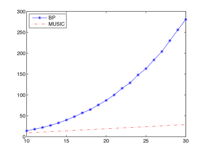
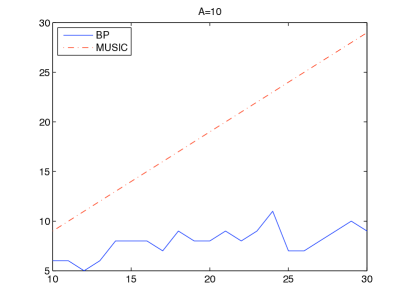
Figure 2. Comparison of MUSIC and BP performances, with both using the whole data matrix: the number $s$ of recoverable scatterers versus the number of sensors $n$ with $A=100$ (left), the well-resolved case, and $A=10$ (right), the under-resolved case. In the well-resolved case, BP delivers a much better (quadratic-in-$n$) performance than MUSIC; in the under-resolved case, MUSIC outperforms BP whose performance tends to be unstable in this regime. The numbers of recoverable scatterers by BP are calculated based on successful recovery of at least 90 out of 100 independent realizations of transceivers and scatterers while the success rate of MUSIC is 100%.

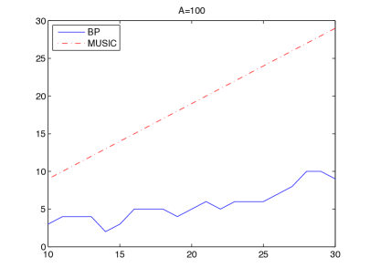
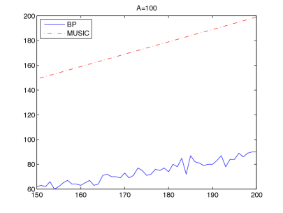
Figure 3. Comparison of MUSIC and BP performances with BP employing only single column of the data matrix: the number $s$ of recoverable scatterers versus the number of sensors $n$ with $A=100$ for $n\in[10,30]$ (left) and $n\in[150,200]$ (right). Both BP curves show a roughly linear behavior with slope less than that of the MUSIC curves.

Figure 2 compares the performances of MUSIC and BP in the well-resolved case $A=100$ and the under-resolved case $A=10$ where the aperture is only one tenth of that satisfying (82). For Figure 2 BP is carried out on the data matrix $\mathbf{Y}$ with the sensors coincident with the sources, i.e. $\mathbf{\Phi}={\mathbf{\Psi}}$. To put the problem in the proper set-up for BP, we vectorize $\mathbf{Y}$ by staking its $n$ columns and denote the resulting $\mathbb{C}^{n^{2}}$ vector by $Y$. We vectorize the diagonal matrix $\tilde{\mathbf{X}}$ by listing its $N$ diagonals as a $\mathbb{C}^{N}$ vector $\tilde{X}$. The BP performance of this set-up has been analyzed in [11]. The numbers of recoverable scatterers shown in Figure 2 are computed for at least $90\%$ recovery rate based on $100$ independent realizations of transceivers and scatterers. In both cases, MUSIC recovers $s=n-1$ scatterers with certainty. Clearly, for the well-resolved case, BP has a far superior performance to MUSIC. Indeed, it can be shown that BP can recover $s=\mathcal{O}(n^{2})$ scatterers with high probability in the well-resolved case [11]. The quadratic behavior is illustrated by the near-parabolic curve in Figure 8(left). For the under-resolved case, however, MUSIC outperforms BP by a significant margin, Figure 8(right). As pointed out in Remark 3, the MUSIC algorithm has the superresolution capability for a sufficiently small noise-to-scatterer ratio.

If only one column of $\mathbf{Y}$ is used in BP as discussed in Section 5, then MUSIC outperforms BP by a wide margin even in the well-resolved case, Figure 3.

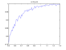
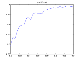
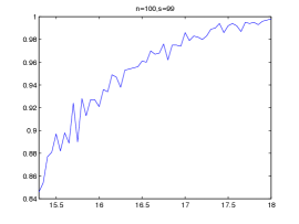
Figure 4. Success probability of the MUSIC reconstruction versus aperture for $n=10,s=9$ (left), $n=100,s=9$ (middle) and $n=100,s=99$ (right). Note the different aperture ranges for the three plots. The success rate is calculated from 1000 trials. Increasing the number of transceivers for the same number of scatterers reduces the aperture required for the same success rate. The reduction of aperture is about three folds (left to middle). On the other hand, higher number of scatterers with the same number of transceivers also demands larger aperture for the same success rate. The increase in aperture is about 7 times (middle to right).

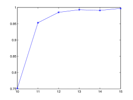
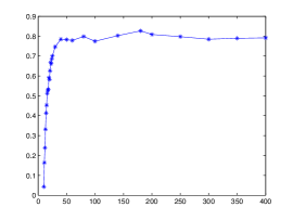
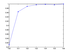
Figure 5. Success probability of MUSIC versus the number of transceivers with $A=0.5,s=9$ (left), $A=0.2,s=9$ (middle) and $A=15,s=99$ (right). The probabilities are calculated from 1000 independent trials.

We further investigate the performance of the MUSIC algorithm for the extremely under-resolved case when BP essentially has extremely low probabilities of exact recovery (even for $s=1$). Figure 4 shows the success probabilities of MUSIC as a function of aperture for various $n$ and $s$ while Figure 5 shows the success probabilities of MUSIC as a function of $n$ for various $A$ and $s$. The success rates are calculated from 1000 independent realizations of transceivers and scatterers.

Three observations about Figure 4 are in order: (i) The optimal performance of $s=n-1$ does not hold with certainty for $s$ relatively large with respect to aperture (cf. left and right panels); (ii) Increasing the number of randomly selected transceivers reduces the aperture required for the same probability of recovering the same number of scatterers (left to middle panels); (iii) Increasing the number of randomly selected scatterers increases the aperture required for the same probability of recovery with the same number of transceivers (middle to right panels).

Likewise, the success rates increase with the number of transceivers for any aperture and sparsity (Figure 5). The most interesting plot in Figure 5 is the middle panel which shows for $A=0.2,s=9$ the success rate curve becomes a plateau after reaching $80\%$. This is not inconsistent with the prediction of Proposition 1 since Proposition 1 assumes a fixed configuration of scatterers while Figure 5 is for random, independent realizations of scatterers. In other words the threshold $n_{0}$ in Proposition 1 may not be uniformly valid for all configurations of $s$ scatterers in the under-resolved case. On the other hand, when the aperture increases by two and half times to $A=0.5$ and the number of transceivers increases to 15, the performance becomes uniform with respect to the scatterer configuration (left panel).

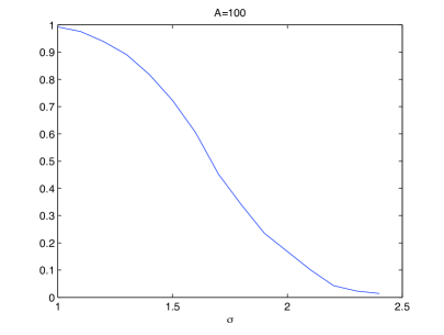
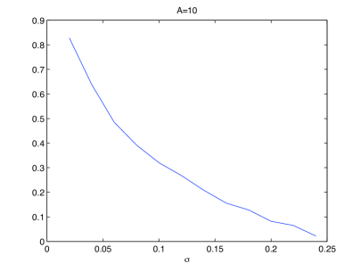
Figure 6. Success probability of MUSIC reconstruction of $s=10$ scatterers with $n=100$ transceivers versus the noise level $\sigma$ in the well-resolved case $A=100$ (left) and the under-resolved case $A=10$ (right). The success rate is calculated from 1000 trials. Note the different scales of $\sigma$ in the two plots. Noise sensitivity increases dramatically in the under-resolved case.

Figure 6 shows the noise sensitivity of MUSIC reconstruction of 10 scatterers with 100 transceivers. Here $n$ and $s$ are chosen so that (75) is roughly satisfied. We add the i.i.d. noises

(103) $$\sigma(e_{1}+ie_{2})Y_{\rm max}$$

to the entries of the unperturbed data matrix where $e_{1}$ and $e_{2}$ are independent, uniform r.v.s in $[-1,1]$ and $Y_{\rm max}$ is the maximum absolute value of the data entries. Hence the signal-to-noise ratio (SNR) is about $2^{-1}\sigma^{-2}$. In the well-resolved case ($A=100$) the MUSIC reconstruction can withstand a significant amount of noise in the data matrix. Indeed, at SNR $0.5$ the success rate is almost $100\%$, consistent with the prediction of Theorem 2, and even at SNR $0.22$ ($\sigma=1.5$) the success rate can be indefinitely improved by increasing the number of transceivers (Figure 7, left panel).

In the under-resolved case, however, the noise sensitivity increases significantly. Figure 6 (right panel) reminds us how fragile the superior performance of MUSIC in the under-resolved case is, cf. Figure 8 (right panel). Figure 7 (right panel) further indicates that in the under-resolved case the success rate may not be indefinitely improved by increasing the number of transceivers in the presence of noise.

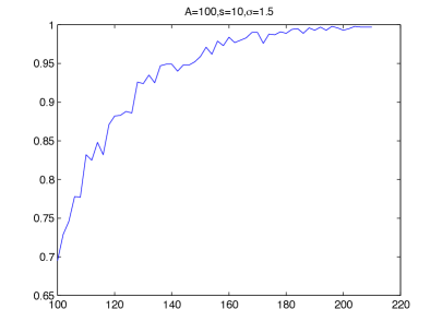
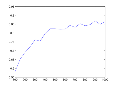
Figure 7. Success probability of MUSIC reconstruction of $s=10$ scatterers as a function of $n$ with $\sigma=150\%$ in the well-resolved case $A=100$ (left) and $\sigma=5\%$ in the under-resolved case $A=10$ (right). The success rate reaches the plateau of $85\%$ near $n=1000$ in the under-resolved case. The success rate is calculated from 1000 trials.

9. Conclusion

We have developed a framework for discrete, quantitative analysis of the MUSIC algorithm in the well-resolved case. Our approach is based on the RIP (40) and its variant (41) which takes into account of the object configuration as well as sparsity.

Our first main result is a support recovery condition (Theorem 2) that for the NOR obeying (59) MUSIC can exactly localize the objects with noisy data. Our result indicates the superresolution capability of the MUSIC algorithm when the noise level is sufficiently low (Remark 3).

We have provided a coherence approach to estimating RIC (Propositions 4 and 3) for general object configuration in three dimensions with the grid spacing $\ell\sim\lambda s$ and the sensor number $n\sim{s^{2}}$. When the scatterers are distributed in a transverse plane, then $\ell\sim\lambda,n\sim s$ (modulo logarithmic factors), suffices. We have extended these results to the gridless setting for which $\ell$ is interpreted as the minimum distance between objects and only approximate localization up to the error $\ell$ is sought (Theorem 5 and Corollary 8).

Our comparative analysis shows that when the whole data matrix is employed in both BP and MUSIC, BP outperforms MUSIC in the well-resolved case in the sense that the number of objects recoverable by BP grows quadratically with the number of transceivers while that by MUSIC grows linearly. The MUSIC reconstruction can tolerate a significant amount of noise in the data matrix (Figures 6, 7, left panels). On the other hand, our numerical results show that in the under-resolved case MUSIC outperforms BP by a wide margin (Figure 2, right panel, Figures 4 and 5). However, MUSIC’s superresolution effect is still unstable with respect to noise in the data matrix (Figures 6, 7, right panels).

Finally, even in the well-resolved case where the employment of just one column of the data matrix by BP guarantees a probabilistic recovery of objects numbered in linear proportion to the number of sensors, analogous to the performance guarantee of MUSIC, the latter outperforms the former in numerical simulations by a wide margin (Figure 3).

Acknowledgement. I am grateful to Mike Yan for preparing the figures and the National Science Foundation for supporting the research through grant DMS 0908535. I thank Wenjing, Liao for pointing out the result, Proposition 2, which helps improve the results of the previous version of the manuscript.

Appendix A Sparse extended objects

Figure 8. Scattering by extended objects

In this appendix we extend the MUSIC algorithm to image sparse extended scatterers by interpolating from grid points.

Suppose that the object function $\xi(\mathbf{r})$ has a compact support. Consider the discrete approximation by interpolating from the grid points

$$\xi_{\ell}(\mathbf{r})=\ell^{2}\sum_{\mathbf{q}\in{\mathcal{I}}}g(\mathbf{r}/\ell-\mathbf{q})\xi(\ell\mathbf{q}),\quad{\mathcal{I}}\subset\mathbb{Z}^{d}$$

where $g$ is some spline function and $\ell$ is the grid spacing. Since $\xi$ has a compact support, ${\mathcal{I}}$ is a finite set. For simplicity assume $d=2$ and let ${\mathcal{I}}$ be the finite lattice

$${\mathcal{I}}=\{\mathbf{q}=(q_{1},q_{2}):q_{1},q_{2}=1,...,\sqrt{N}\}$$

of total cardinality $N$ and ${\mathcal{K}}=\ell{\mathcal{I}}$. In the case of a characteristic function $g$, $\xi_{l}$ is a piece-wise constant object function. We will neglect the discretization error and assume $\xi_{\ell}(\mathbf{r})=\xi(\mathbf{r})$ in the subsequent analysis.

The data matrix $\mathbf{Y}\in\mathbb{C}^{n\times m}$ is given by

$$Y_{k,l} \sim {\ell^{d}}\sum_{\mathbf{q}\in I}\xi(\ell\mathbf{q})\int_{\mathbb{R}^{d}}g(\mathbf{r}^{\prime}/\ell-\mathbf{q})e^{i\omega(\hat{\mathbf{d}}_{l}-\hat{\mathbf{s}}_{k})\cdot\mathbf{r}^{\prime}}d\mathbf{r}^{\prime},$$

$$= {\ell^{d}(2\pi)^{d/2}}\hat{g}(\ell\omega(\hat{\mathbf{d}}_{l}-\hat{\mathbf{s}}_{k}))\sum_{\mathbf{q}\in I}\xi(\ell\mathbf{q})e^{i\omega\ell(\hat{\mathbf{d}}_{l}-\hat{\mathbf{s}}_{k})\cdot\mathbf{q}}.$$

As before we maintain the option of normalizing $\mathbf{Y}$. Suppose $\{\xi_{j}=\xi(\ell\mathbf{q}_{j}):j=1,...,s\}$ is the set of nonvanishing $\xi(\ell\mathbf{q})$ and let $\mathbf{X}=\hbox{\rm diag}(\xi_{j})\in\mathbb{C}^{s\times s}$. Dividing (A) by ${\ell^{d}(2\pi)^{d/2}}\hat{g}(\ell\omega(\hat{\mathbf{d}}_{l}-\hat{\mathbf{s}}_{k}))/2$ we can write the data matrix in the form (10) with the sensing matrices

$$\Phi_{kj} = {1\over\sqrt{n}}e^{-i\omega\ell\hat{\mathbf{s}}_{k}\cdot\mathbf{q}}\in\mathbb{C}^{n\times s}$$

$$\Psi_{lj} = {1\over\sqrt{n}}e^{-i\omega\ell\hat{\mathbf{d}}_{l}\cdot\mathbf{q}}\in\mathbb{C}^{n\times s}$$

where $j=(q_{1}-1)\sqrt{N}+q_{2}$.

In other words, the scattering analysis for both point and extended scatterers leads to the same type of Fourier-like matrices.

Appendix B Proof of Theorem 3

The following lemma differs from the original version in [2].

Lemma 5.

We have

$$\left|\Re\left\langle\tilde{\mathbf{\Phi}}Z,\tilde{\mathbf{\Phi}}Z^{\prime}\right\rangle\right|\leq{1\over 2}\left(\delta^{+}_{s+s^{\prime}}+\delta_{s+s^{\prime}}^{-}\right)\|Z\|_{2}\|Z^{\prime}\|_{2}$$

for all $Z,Z^{\prime}$ supported on disjoint subsets $T,T^{\prime}\subset\{1,...,m\}$ with $|S|\leq s,|S^{\prime}|\leq s^{\prime}.$

Proof.

Without loss of generality, suppose $Z,Z^{\prime}$ are unit vectors. Since $Z\perp Z^{\prime}$, $\|Z\pm Z^{\prime}\|^{2}_{2}=2.$ Hence we have from the RIP (40)

(105) $$2(1-\delta^{-}_{s+s^{\prime}})\leq\|\tilde{\mathbf{\Phi}}(Z\pm Z^{\prime})\|_{2}^{2}\leq 2(1+\delta^{+}_{s+s^{\prime}})$$

By the parallelogram identity and (105)

$$\left|\Re\left\langle\tilde{\mathbf{\Phi}}Z,\tilde{\mathbf{\Phi}}Z^{\prime}\right\rangle\right|={1\over 4}\left|\|\tilde{\mathbf{\Phi}}Z+\tilde{\mathbf{\Phi}}Z^{\prime}\|_{2}^{2}-\|\tilde{\mathbf{\Phi}}Z-\tilde{\mathbf{\Phi}}Z^{\prime}\|_{2}^{2}\right|\leq{1\over 2}\left(\delta^{+}_{s+s^{\prime}}+\delta_{s+s^{\prime}}^{-}\right)$$

which proves the lemma. ∎

By the triangle inequality and the fact that $Z$ is in the feasible set we have

(106) $$\|\tilde{\mathbf{\Phi}}(\hat{Z}-Z)\|_{2}\leq\|\tilde{\mathbf{\Phi}}\hat{Z}-Y\|_{2}+\|Y-\tilde{\mathbf{\Phi}}Z\|_{2}\leq 2\varepsilon.$$

Set $\hat{Z}=Z+\Delta$ and decompose $\Delta$ into a sum of vectors $\Delta_{S_{0}},\Delta_{S_{1}},\Delta_{S_{2}},...,$ each of sparsity at most $s$. Here $S_{0}$ corresponds to the locations of the $s$ largest coefficients of $Z$; $S_{1}$ to the locations of the $s$ largest coefficients of $\Delta_{S_{0}^{c}}$; $S_{2}$ to the locations of the next $s$ largest coefficients of $\Delta_{S_{0}^{c}}$, and so on.

Step (i). For $j\geq 2$,

$$\|\Delta_{S_{j}}\|_{2}\leq s^{1/2}\|\Delta_{S_{j}}\|_{\infty}\leq s^{-1/2}\|\Delta_{S_{j-1}}\|_{2}$$

and hence

(107) $$\sum_{j\geq 2}\|\Delta_{S_{j}}\|_{2}\leq s^{-1/2}\sum_{j\geq 1}\|\Delta_{S_{j}}\|_{1}\leq s^{-1/2}\|\Delta_{S_{0}^{c}}\|_{1}.$$

This yields

(108) $$\|\Delta_{(S_{0}\cup S_{1})^{c}}\|_{2}=\|\sum_{j\geq 2}\Delta_{S_{j}}\|_{2}\leq\sum_{j\geq 2}\|\Delta_{S_{j}}\|_{2}\leq s^{-1/2}\|\Delta_{S_{0}^{c}}\|_{1}.$$

Also we have

$$\|Z\|_{1}\geq\|\hat{Z}\|_{1}=\|Z_{S_{0}}+\Delta_{S_{0}}\|_{1}+\|Z_{S_{0}^{c}}+\Delta_{S_{0}^{c}}\|_{1}\geq\|Z_{S_{0}}\|_{1}-\|\Delta_{S_{0}}\|_{1}-\|Z_{S_{0}^{c}}\|_{1}+\|\Delta_{S_{0}^{c}}\|_{1}$$

which implies

(109) $$\|\Delta_{S_{0}^{c}}\|_{1}\leq 2\|Z_{S_{0}^{c}}\|_{1}+\|\Delta_{S_{0}}\|_{1}.$$

Note that $\|Z_{S_{0}^{c}}\|_{1}=\|Z-Z^{(s)}\|_{1}$ by definition. Applying (108), (109) and the Cauchy-Schwarz inequality gives

(110) $$\|\Delta_{(S_{0}\cup S_{1})^{c}}\|_{2}\leq\|\Delta_{S_{0}}\|_{2}+2e_{0}$$

where $e_{0}\equiv s^{-1/2}\|Z-Z^{(s)}\|_{1}$.

Step (ii). Observe

$$\|\tilde{\mathbf{\Phi}}\Delta_{S_{0}\cup S_{1}}\|_{2}^{2} = \left\langle\tilde{\mathbf{\Phi}}\Delta_{S_{0}\cup S_{1}},\tilde{\mathbf{\Phi}}\Delta\right\rangle-\left\langle\tilde{\mathbf{\Phi}}\Delta_{S_{0}\cup S_{1}},\sum_{j\geq 2}\tilde{\mathbf{\Phi}}\Delta_{S_{j}}\right\rangle$$

$$= \Re\left\langle\tilde{\mathbf{\Phi}}\Delta_{S_{0}\cup S_{1}},\tilde{\mathbf{\Phi}}\Delta\right\rangle-\sum_{j\geq 2}\Re\left\langle\tilde{\mathbf{\Phi}}\Delta_{S_{0}\cup S_{1}},\tilde{\mathbf{\Phi}}\Delta_{S_{j}}\right\rangle$$

$$= \Re\left\langle\tilde{\mathbf{\Phi}}\Delta_{S_{0}\cup S_{1}},\tilde{\mathbf{\Phi}}\Delta\right\rangle-\sum_{j\geq 2}\left[\Re\left\langle\tilde{\mathbf{\Phi}}\Delta_{S_{0}},\tilde{\mathbf{\Phi}}\Delta_{S_{j}}\right\rangle+\Re\left\langle\tilde{\mathbf{\Phi}}\Delta_{S_{1}},\tilde{\mathbf{\Phi}}\Delta_{S_{j}}\right\rangle\right].$$

This calculation differ slightly from the corresponding calculation in [2].

From (106) and the RIP (40) it follows that

$$\|\left\langle\tilde{\mathbf{\Phi}}\Delta_{S_{0}\cup S_{1}}\right\rangle\|\leq\|\tilde{\mathbf{\Phi}}\Delta_{S_{0}\cup S_{1}}\|_{2}\|\tilde{\mathbf{\Phi}}\Delta\|_{2}\leq 2\varepsilon\sqrt{1+\delta^{+}_{2s}}\|\Delta_{S_{0}\cup S_{1}}\|_{2}.$$

Moreover, it follows from Lemma B that

$$\left|\Re\left\langle\tilde{\mathbf{\Phi}}\Delta_{S_{0}},\tilde{\mathbf{\Phi}}\Delta_{S_{j}}\right\rangle\right| \leq {1\over 2}\left(\delta^{+}_{2s}+\delta^{-}_{2s}\right)\|\Delta_{S_{0}}\|_{2}\|\Delta_{S_{j}}\|_{2}$$

$$\left|\Re\left\langle\tilde{\mathbf{\Phi}}\Delta_{S_{1}},\tilde{\mathbf{\Phi}}\Delta_{S_{j}}\right\rangle\right| \leq {1\over 2}\left(\delta^{+}_{2s}+\delta^{-}_{2s}\right)\|\Delta_{S_{0}}\|_{2}\|\Delta_{S_{j}}\|_{2}$$

for $j\geq 2$. Since $S_{0}$ and $S_{1}$ are disjoint

$$\|\Delta_{S_{0}}\|_{2}+\|\Delta_{S_{1}}\|_{2}\leq\sqrt{2}\sqrt{\|\Delta_{S_{0}}\|^{2}_{2}+\|\Delta_{S_{1}}\|^{2}_{2}}=\sqrt{2}\|\Delta_{S_{0}\cup S_{1}}\|_{2}.$$

Also

$$(1-\delta^{-}_{2s})\|\Delta_{S_{0}\cup S_{1}}\|_{2}^{2}\leq\|\tilde{\mathbf{\Phi}}\Delta_{S_{0}\cup S_{1}}\|_{2}^{2}\leq\|\Delta_{S_{0}\cup S_{1}}\|_{2}\left(2\varepsilon\sqrt{1+\delta^{+}_{2s}}+{1\over\sqrt{2}}\left(\delta^{+}_{2s}+\delta^{-}_{2s}\right)\sum_{j\geq 2}\|\Delta_{S_{j}}\|_{2}\right).$$

Therefore from (107) we obtain

$$\|\Delta_{S_{0}\cup S_{1}}\|_{2}\leq\alpha\varepsilon+\rho s^{-1/2}\|\Delta_{S_{0}^{c}}\|_{1},\quad\alpha={2\sqrt{1+\delta^{+}_{2s}}\over 1-\delta^{-}_{2s}},\quad\rho={{1\over\sqrt{2}}\left(\delta^{+}_{2s}+\delta^{-}_{2s}\right)\over 1-\delta^{-}_{2s}}$$

and moreover by (109)

$$\|\Delta_{S_{0}\cup S_{1}}\|_{2}\leq\alpha\varepsilon+\rho\|\Delta_{S_{0}^{c}}\|_{2}+2\rho e_{0}.$$

Namely,

$$\|\Delta_{S_{0}\cup S_{1}}\|_{2}\leq(1-\rho)^{-1}(\alpha\varepsilon+2\rho e_{0})$$

if (86) holds.

Finally,

$$\|\Delta\|_{2}\leq\|\Delta_{S_{0}\cup S_{1}}\|_{2}+\|\Delta_{(S_{0}\cup S_{1})^{c}}\|_{2}\leq 2\|\Delta_{S_{0}\cup S_{1}}\|_{2}+2e_{0}\leq 2(1-\rho)^{-1}(\alpha\varepsilon+(1+\rho)e_{0})$$

which is what we set out to show.

References

[1]
A.M. Bruckstein, D.L. Donoho and M. Elad,
“From sparse solutions of systems of equations to
sparse modeling of signals,” SIAM Rev.51 (2009), 34-81.
[2]
E. J. Candès, “The restricted isometry property and its implications for compressed sensing,” Compte Rendus de l’Academie des Sciences, Paris, Serie I.346 (2008) 589-592.
[3]
E. J. Candès and T. Tao, “ Decoding by linear programming,” IEEE Trans. Inform. Theory51 (2005), 4203 4215.
[4]
S. S. Chen, D. L. Donoho, and M. A. Saunders, Atomic decomposition by basis pursuit, SIAM J. Scientific Comput.
20 (1998), pp. 33 61.
[5]
M. Cheney, “The linear sampling method and
MUSIC algorithm,” Inverse Problems17 (2001), 591-596.
[6]
A. J. Devaney, Super-resolution processing of multi-static data using
time reversal and MUSIC, unpublished manuscript, 2000.
[7]
A. J. Devaney, E. A. Marengo, and F. K. Gruber,
“
Time-reversal-based imaging and inverse scattering of multiply
scattering point objects”,
J. Acoust. Soc. Am. 118 (2005) 3129-3138.
[8]
D.L. Donoho, M. Elad and V.N. Temlyakov,
“Stable recovery of sparse overcomplete
representations in the presence of noise,”
IEEE Trans. Inform. Theory52 (2006) 6-18.
[9]
A. Fannjiang, “Compressive inverse scattering I. High frequency SIMO/MISO and MIMO measurements, ” Inverse Probl.26 (2010), 035008.
[10]
A. Fannjiang, ”Compressive inverse scattering II. Multi-shot SISO measurements with Born scatterers”,
Inverse Probl.26 (2010), 035009.
[11]
A. Fannjiang, P. Yan and Thomas Strohmer,
“Compressed remote sensing of sparse objects,”
arXiv:0904.3994.
[12] F.K. Gruber, E.A. Marengo and A.J. Devaney,
“Time-reversal imaging with multiple signal classification
considering multiple scattering between the objects”,
J. Acoust. Soc. Am.115 (6) (2004), 3042-3047.
[13]
R.A. Horn and C.R. Johnson, Matrix Analysis.
Cambridge University Press, Cambridge, 1985.
[14]
S. Jaffard, Y. Meyer and R.D. Ryan, Wavelets – Tools for Science & Technology. SIAM, Philadelphia, 2001.
[15]
A. Kirsch, “The MUSIC-algorithm and the factorization method
in inverse scattering theory for inhomogeneous media,” Inverse Probl.18 (2002), 1025-1040
[16]
A. Kirsch and N. Grinsberg, The Factorization Method
for Inverse Problems, Oxford University Press, Oxford, 2008.
[17]
C. Prada, and J.-L. Thomas,
“Experimental subwavelength localization of scatterers
by decomposition of the time reversal operator interpreted
as a covariance matrix,” J. Acoust. Soc. Am. 114 (2003), 235-243.
[18]
H. Rauhut, “Stability results for random sampling of sparse trigonometric polynomials,” IEEE Trans. Inform. Th.54 (2008), 5661-5670.
[19]
R. Schmidt, “ Multiple emitter location and signal parameter estimation,” IEEE Trans. Antennas
Propag.34(3) (1986), 276 280.
[20]
G. W. Stewart, J.-G. Sun, Matrix Perturbation Theory, Academic Press, 1990.
[21]
C.W. Therrien, Discrete Random Signals and Statistical Signal Processing (Englewood Cliffs, NJ: Prentice-
Hall), 1992.
[22]
J. Yang and Y. Zhang, “Alternating direction algorithms for
-problems in compressive sensing”, preprint, 2009.