Knot polynomial invariants in classical Abelian Chern-Simons field theory

Abstract

Kauffman knot polynomial invariants are discovered in classical abelian Chern-Simons field theory. A topological invariant $t^{I\left(\mathcal{L}\right)}$ is constructed for a link $\mathcal{L}$, where $I$ is the abelian Chern-Simons action and $t$ a formal constant. For oriented knotted vortex lines, $t^{I}$ satisfies the skein relations of the Kauffman R-polynomial; for un-oriented knotted lines, $t^{I}$ satisfies the skein relations of the Kauffman bracket polynomial. As an example the bracket polynomials of trefoil knots are computed, and the Jones polynomial is constructed from the bracket polynomial.

Keywords: Kauffman polynomials; classical Chern-Simons field theory; knotted vortex lines.

PACS numbers: 11.15.Kc, 02.10.Kn, 02.40.Hw

1 Introduction

Quantum Chern-Simons (CS) theories are one of the most important three-dimensional topological quantum field theories. Witten discovered that [1] quantum CS theories provide a natural field theoretical origin for link invariants, beyond their algebraic origin from quantum groups [2]. Link invariants are the central concept of knot theory used to classify knot equivalence classes; since three-manifolds are related to knots via Dehn surgery, link invariants also yield three-manifold topological invariants. Building on Witten’s breakthrough, considerable knot and three-manifold invariants have been constructed [3, 4]. They can be organised using the Kontsevich integral, and will lead to perturbative CS theories with every term containing a finite type LMO invariants [5]. Recent developments include the Rozansky-Witten model [6, 7] and the Gaiotto-Witten-Kapustin-Saulina model [8], which are constructed to act as the Grassmann-odd versions of the CS actions respectively with normal and super Lie gauge groups. In comparison with CS theories, in these models a large number of terms are dropped from the CS perturbative expansions and hence computation is simplified and elementary information is extracted.

However, for classical CS theories, there are no such direct relationships between link invariants and CS theories. Classical CS theories are based on the CS action, which bears different meaning in various physical problems — a most important example is the helicity in fluid mechanics. Moffatt introduced the concept of helicity and revealed its conservation during evolution of fluid flow [9]. Arnol’d showed that helicity is invariant under volume-preserving diffeomorphisms [10]. Moffatt and Ricca discovered that for a magnetic fluid containing knotted magnetic lines of force its helicity can be given by self-linking and linking numbers of knots [9, 11]. This provides an algebraic method to count magnetic fluid helicity, much simpler than computation of CS $3$-form integrals. Today helicity is important in research of knotted vortex lines in optical beams, Bose-Einstein condensates, magnetohydrodynamics of solar plasma and so on. However, as mentioned, in the study of classical CS theories we still need to find direct relationships between the CS theories and link polynomial invariants, the powerful tool of knot theory for classification of knot equivalence classes, as happened in the case of quantum CS theories. In this regard in this paper we attempt to find polynomial invariants associated to knotted vortex lines in the framework of classical CS theories.

The abelian Chern-Simons action is given by

$$I=\frac{1}{4\pi}\int_{M}A\wedge F=\frac{1}{8\pi}\int_{M}\epsilon^{ijk}A_{i}F_{jk}d^{3}x.$$ (1)

Here $A_{i}$ is a $U\left(1\right)$ gauge potential and $F_{ij}=\partial_{i}A_{j}-\partial_{j}A_{i}$ the field tensor. In the hydrodynamical formulism of quantum mechanics, $A_{i}$ is the velocity field distributed within a quantum fluid, $F_{ij}$ is the vorticity, and $I$ the fluid helicity up to dimensional constants. $A_{i}$ is defined as $A_{i}=\frac{1}{2i\psi^{\ast}\psi}\left(\psi^{\ast}\partial_{i}\psi-\partial_{i}\psi^{\ast}\psi\right)$ in terms of the complex scalar wave function $\psi\left(\vec{x}\right)$ describing the physical system, $\psi=\phi^{1}+i\phi^{2}$, with $\phi^{a}\in\mathbb{R}$, $a=1,2$. Defining a two-dimensional unit vector $n^{a}$ from $\phi^{a}$, $n^{a}=\frac{\phi^{a}}{\left\|\phi\right\|}$, the potential $A_{i}$ can be expressed as

$$A_{i}=\epsilon^{ab}n^{a}\partial_{i}n^{b}.$$ (2)

The field tensor $F_{ij}$ has a quantum mechanical expression in terms of $n^{a}:F_{ij}=2\epsilon^{ab}\partial_{i}n^{a}\partial_{j}n^{b}$. It can be proved that [12] there is a $\delta$-function residing in $F_{ij}:$ $\frac{1}{8\pi}\epsilon^{ijk}F_{jk}=\delta^{2}\left(\phi\right)D^{i}\left(\frac{\phi}{x}\right)$, where $D^{i}\left(\frac{\phi}{x}\right)=\frac{1}{2}\epsilon^{ijk}\epsilon^{ab}\partial_{j}\phi^{a}\partial_{k}\phi^{b}$ is a Jacobian determinant, and $\delta^{2}\left(\phi\right)$ is the $\delta$-function which does not vanish only at zero-points of $\phi^{a}$ (i.e., at singular points of $n^{a}$). The field tensor $F_{ij}$ is non-trivial only at where the zero-point equations, $\phi^{1,2}\left(\vec{x}\right)=0,$ are satisfied. In the three-dimensional real space the solutions to the two zero-point equations are a family of, say, $N$ isolated singular line structures. These lines are just the vortex lines arising from singularity of the field tensor $F_{ij}$. Let $\xi_{k}$ denote the $k$-th line with a parametric equation $x^{i}=z_{k}^{i}\left(s\right),\$where $s$ is the line parameter. Locally, the unit vector $n^{a}$ lies in the two-dimensional plane normal to $\xi_{k}$, with the intersection point between $\xi_{k}$ and the plane being the singular point of the $n^{a}$ field. Then $\delta^{2}\left(\phi\right)$ can be expanded onto these $N$ lines as $\delta^{2}\left(\phi\right)D^{i}\left(\frac{\phi}{x}\right)=\sum_{k=1}^{N}W_{k}\int_{\xi_{k}}\frac{dx^{i}}{ds}\delta^{3}\left(\vec{x}-\vec{z}_{k}\left(s\right)\right)ds,$ where $W_{k}$ is the topological charge of $\xi_{k}$. In hydrodynamics $W_{k}$ may carry the meaning of fluid flux. Thus the CS action becomes $I=\frac{1}{2\pi}\sum_{k=1}^{N}W_{k}\int_{\xi_{k}}A_{i}dx^{i}.$ Especially, when the vortex lines are $N$ closed knots forming a link $\mathcal{L}$, the CS action $I$ becomes a sum of integrals over $\mathcal{L}$:

$$I\left(\mathcal{L}\right)=\frac{1}{2\pi}\sum_{k=1}^{N}W_{k}\oint_{\xi_{k}}A_{i}dx^{i}.$$ (3)

In [12] we analysed the CS action by means of gauge potential decomposition and showed that $I$ is closely related to (self-)linkage of the knots of $\mathcal{L}$:

$$I\left(\mathcal{L}\right)=\sum_{k=1}^{N}W_{k}^{2}Sl\left(\xi_{k}\right)+\sum_{k,l=1;k\neq l}^{N}W_{k}W_{l}Lk\left(\xi_{k},\xi_{l}\right),$$ (4)

where $Sl\left(\xi_{k}\right)$ is the self-linking number of one knot $\xi_{k}$, and $Lk\left(\xi_{k},\xi_{l}\right)$ the linking number between two knots $\xi_{k}$ and $\xi_{l}$. Eq.(4) is consistent with the conclusion of Moffatt et al. [11].

For the discussions in the following sections it is worth here having a quick revisit to our analysis of [12] for (3) and (4), as follows. Introduce a $3$-dimensional unit vector $\vec{m}=\frac{\vec{\kappa}-\vec{\zeta}}{\left\|\vec{\kappa}-\vec{\zeta}\right\|},$ where $\vec{\kappa}$ and $\vec{\zeta}$ are two points respectively picked up from two knots $\xi_{k}$ and $\xi_{l}$ of the link $\mathcal{L}$. When $\vec{\kappa}$ and $\vec{\zeta}$ run along knots of $\mathcal{L}$, the $\vec{m}$ runs over the $2$-dimensional sphere $S^{2}$ in the $3$-dimensional space. On this $S^{2}$ we introduce a unit vector $e^{A}$, with $A=1,2$ denoting the local coordinates on $S^{2}$. Apparently $\vec{e}$ is always perpendicular to $\vec{m}$. In [12] the $\vec{e}$ is used to re-express the gauge potential $A_{i}$ as $A_{i}=\epsilon^{AB}e^{A}\partial_{i}e^{B}$, hence (3) becomes $I\left(\mathcal{L}\right)=\frac{1}{2\pi}\sum_{k=1}^{N}W_{k}\oint_{\xi_{k}}\epsilon^{AB}e^{A}\partial_{i}e^{B}d\kappa^{i}$. With the consideration that $m^{i}$ is defined from both $\xi_{k}$ and $\xi_{l}$, we write $I\left(\mathcal{L}\right)$ more symmetrically as

$$I\left(\mathcal{L}\right)=\frac{1}{4\pi}\sum_{k,l=1}^{N}W_{k}W_{l}\oint_{\xi_{k}}d\kappa^{i}\oint_{\xi_{l}}d\zeta^{j}\epsilon^{AB}\partial_{i}e^{A}\partial_{j}e^{B}.$$ (5)

Now let us investigate (5) by examining the two points $\vec{\kappa}$ and $\vec{\zeta}$. Eq.(5) contains three cases in regard to different relative positions of $\vec{\kappa}$ and $\vec{\zeta}$: (i) $\xi_{k}$ and $\xi_{l}$ are different knots and $\vec{\kappa}$ and $\vec{\zeta}$ are different points; (ii) $\xi_{k}$ and $\xi_{l}$ are a same knot but $\vec{\kappa}$ and $\vec{\zeta}$ are different points; (iii) $\vec{\kappa}$ and $\vec{\zeta}$ are a same point.

• Case (i): In regard to the definitions of $\vec{m}$ and $\vec{e}$, we see that $\epsilon^{AB}e^{A}\partial_{i}e^{B}$ indeed gives a Wu-Yang potential [13]. Hence (5) leads to $I\left(\mathcal{L}\right)_{\mathrm{(i)}}=\sum_{k,l=1;k\neq l}^{N}\frac{W_{k}W_{l}}{4\pi}\oint_{\xi_{k}}d\kappa^{i}\oint_{\xi_{l}}d\zeta^{j}\left(\vec{m}\cdot\partial_{i}\vec{m}\times\partial_{j}\vec{m}\right)$, where $\vec{m}\cdot\partial_{i}\vec{m}\times\partial_{j}\vec{m}$ is recognized to be a surface element of the $S^{2}$. According to [14], $I\left(\mathcal{L}\right)_{\mathrm{(i)}}$ presents the linking number between $\xi_{k}$ and $\xi_{l}:I\left(\mathcal{L}\right)_{\mathrm{(i)}}=\sum_{k,l=1;k\neq l}^{N}W_{k}W_{l}Lk\left(\xi_{k},\xi_{l}\right)$.

• Case (ii): Similarly, the integral of (5) leads to the writhing number $Wr\left(\xi_{k}\right)$ of the knot $\xi_{k}$: $I\left(\mathcal{L}\right)_{\mathrm{(ii)}}=\sum_{k=1}^{N}W_{k}^{2}Wr\left(\xi_{k}\right)$.

• Case (iii): In this case $\vec{m}$ becomes the tangent vector $\vec{T}$ of the vortex line $\xi_{k}$. And $\vec{e}$ becomes the vector normal to $\vec{T}$, having arbitrariness of rotating about $\vec{T}$. On the one hand, according to differential geometry of curves, $\xi_{k}$ possesses a Frenet frame formed by three orthonormal vectors: $\vec{T}$, $\vec{N}$ and $\vec{B}$, where $\vec{N}$ and $\vec{B}$ are the so-called normal and bi-normal unit vectors. On the other hand, for the decomposition (2) of the $U\left(1\right)$ potential $A_{i}$, on a plane normally intersecting $\xi_{k}$ the intersection point is a singular ill-defined point of the $\vec{n}$ field. Then, noticing $\vec{n}$ is in the same plane containing $\vec{e}$, the singularity of the $\vec{n}$ field can be removed by redefining on $\xi_{k}$

  $$\vec{n}\equiv\vec{e}\equiv\vec{N}.$$ (6)

  Then the double integral (5) reduces to a single integral $I\left(\mathcal{L}\right)_{\mathrm{(iii)}}$ $=\frac{1}{2\pi}\sum_{k=1}^{N}W_{k}^{2}\oint_{\xi_{k}}\epsilon^{ab}n^{a}\partial_{i}n^{b}d\kappa^{i}$ $=\frac{1}{2\pi}\sum_{k=1}^{N}W_{k}^{2}Tw\left(\xi_{k}\right)$, yielding the twisting number of $\xi_{k}$, $Tw\left(\xi_{k}\right)=\oint_{\xi_{k}}\vec{N}\cdot d\vec{B}$.

Thus, in the light of the Calugareanu-White formula $Sl\left(\xi_{k}\right)=Wr\left(\xi_{k}\right)+Tw\left(\xi_{k}\right)$, one can summarize Cases (i)–(iii) to obtain the above result (4):

$$I\left(\mathcal{L}\right)=I\left(\mathcal{L}\right)_{\mathrm{(i)}}+I\left(\mathcal{L}\right)_{\mathrm{(ii)}}+I\left(\mathcal{L}\right)_{\mathrm{(iii)}}=\sum_{k=1}^{N}W_{k}^{2}Sl\left(\xi_{k}\right)+\sum_{k,l=1;k\neq l}^{N}W_{k}W_{l}Lk\left(\xi_{k},\xi_{l}\right).$$ (7)

Here a point should be emphasized. It is seen that in Cases (i) and (ii) the points $\vec{\kappa}$ and $\vec{\zeta}$ are different, no matter the knots $\xi_{k}$ and $\xi_{l}$ are different or not. Therefore, Case (i) plus (ii) indeed wrap up all the contributions of “different-point-defined $\vec{m}$” to $I\left(\mathcal{L}\right)$. This fact will play an important role in the next section.

In this paper we will further study deeper algebraic essence of $I\left(\mathcal{L}\right)$ and reveal its relationship to the polynomial invariants of knot theory. Significance of this study dwells in that it establishes a bridge between the CS action and algebraic polynomial invariants of knot theory. The paper is arranged as follows. In Section 2 the skein relations of the Kauffman R-polynomial for oriented knotted vortex lines will be obtained. In Section 3 the skein relations of the Kauffman bracket polynomial for un-oriented knotted lines will be obtained. As an example the bracket polynomials of trefoil knots will be computed, and the well-known Jones polynomial will be constructed from the bracket polynomial. Our emphasis is to be placed on Section 3. In Section 4 the paper will be summarized and discussions be presented.

Before proceeding, a preparation should be addressed. Since crossing and writhing of vortex lines are to be discussed below, vortex lines should have same topological charges, otherwise the discussion cannot be conducted. Hence in this paper all topological charges of vortex lines take a same value: $W_{1}=\cdots=W_{N}=W$. For convenience, one evaluates $W=1$.

2 Kauffman R-polynomial invariant for oriented knots

We argue that the exponential

$$t^{H\left(\mathcal{L}\right)}=t^{\frac{1}{2\pi}\sum_{k}\oint_{\xi_{k}}A_{i}dx^{i}}$$ (8)

is capable to present the Kauffman R-polynomial for oriented knotted vortex lines and present the Kauffman bracket polynomial for un-oriented knotted vortex lines. Here $t$ is a constant, which will appear formally in the following deduction and may be determined when compared to, say, a concrete fluid mechanical model. If the theory of this paper could be applied in another physical problem, which possesses the Chern-Simons-type action (1), then $t$ would bear a different physical meaning in that circumstance.

In this section the R-polynomial for oriented knots will be studied. Oriented knots are useful in solving some physical problems. For instance, the tangled open vortex lines in Figure 1 can be conveniently studied if they are regarded as oriented knots:

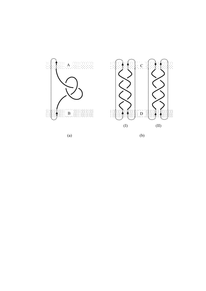
Figure 1: Tangled open vortex lines can be studied as oriented knots.

• In Figure 1(a), to study the tangled line: firstly, one can extend the open ends at the different boundaries $A$ and $B$ to infinity, and trivially connect them with the dashed curve to form a closed loop; secondly, to distinguish $A$ and $B$ a convenient way is to endow the line with an orientation. Thus the open vortex line can be studied as an oriented knot;

• In Figure 1(b), consider two braids of open vortex lines which are in different intertwining configurations, respectively marked as (I) and (II). To distinguish them a reasonable way is: firstly, in each braid, to connect the open ends at the different boundaries $C$ and $D$ with the dashed curves shown; secondly, to endow each line with an orientation to distinguish $C$ and $D$. Thus, the different tangles (I) and (II) can be studied as two oriented knots.

For the purpose of obtaining the R-polynomial from $t^{I\left(\mathcal{L}\right)}$, crossing and writhing configurations of links should be studied: for crossing, consider three links which are almost the same except at one particular point where different crossing situations occur, as shown in Figure 2(a) to 2(c). The very point $X$ is called a double point, and the over-crossing, under-crossing and non-crossing links are respectively denoted by $l_{+},\ l_{-}$ and $l_{0}$; for writhing, one uses $\hat{l}_{+},\ \hat{l}_{-}$ and $\hat{l}_{0}$ to denote three links which are almost the same except for different writhing situations at the point $X$, as shown in Figure 2(d) to 2(f).

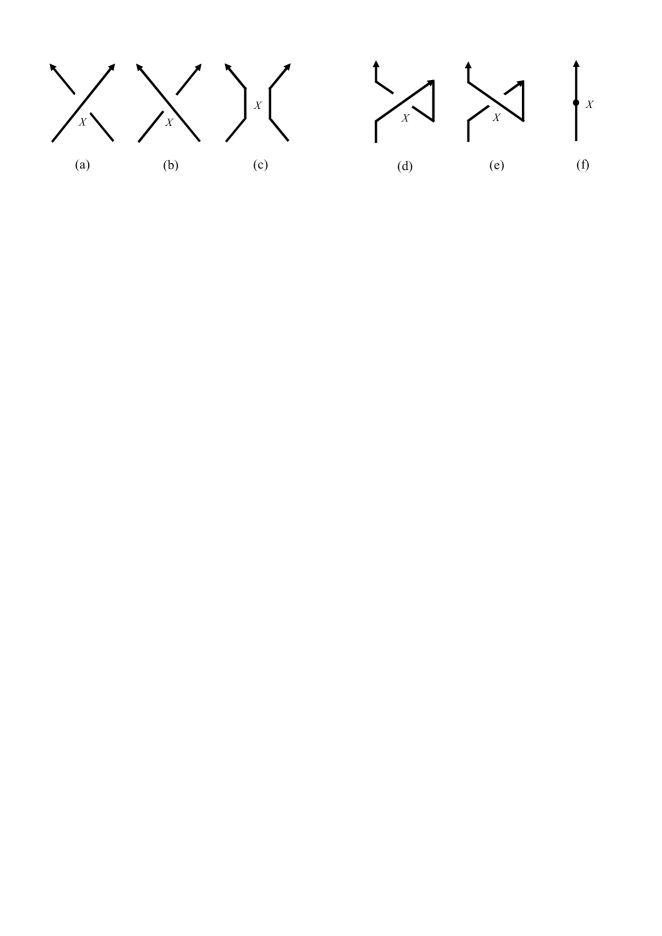
Figure 2: Crossing configurations of oriented knots: (a) $l_{+}$; (b) $l_{-}$; (c) $l_{0}$. Writhing configurations of oriented knots: (d) $\hat{l}_{+}$; (e) $\hat{l}_{-}$; (f) $\hat{l}_{0}$.

Now let us examine $t^{I\left(\hat{l}_{+}\right)}$, $t^{I\left(\hat{l}_{-}\right)}$ and $t^{I\left(\hat{l}_{0}\right)}$. Since the vortex lines are oriented, the integration paths can be re-expressed as:

$$\hat{l}_{+}=\hat{l}_{0}\oplus\gamma_{+}^{\phantom{.}\prime}=\hat{l}_{0}\oplus\gamma_{+},\ \ \ \ \ \ \ \ \ \hat{l}_{-}=\hat{l}_{0}\oplus\gamma_{-}^{\phantom{.}\prime}=\hat{l}_{0}\oplus\gamma_{-},$$ (9)

where the symbol “$\oplus$” means “union after imaginarily adding and subtracting paths”, and $\gamma_{+},\ \gamma_{+}^{\phantom{.}\prime},\ \gamma_{-}$ and $\gamma_{-}^{\phantom{.}\prime}$ are shown in Figure 3(a), 3(b), 3(d) and 3(e) respectively. For these imaginary paths we require that

$$t^{I\left(\hat{l}_{\pm}\right)}=t^{I\left(\hat{l}_{0}\oplus\gamma_{\pm}\right)}=t^{I\left(\gamma_{\pm}\right)}t^{I\left(\hat{l}_{0}\right)},$$ (10)

which demonstrates the difference between the writhing $\hat{l}_{\pm}$ and the non-writhing $\hat{l}_{0}$.

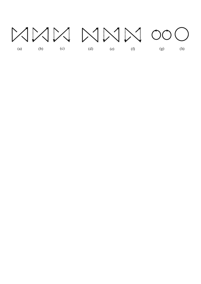
Figure 3: Configurations used in the study of oriented knots: (a) $\gamma_{+}$; (b) $\gamma_{+}^{\prime}$, containing one imaginarily added segment; (c) $\gamma_{+}^{\prime\prime}$, containing two imaginarily added segments; (d) $\gamma_{-}$; (e) $\gamma_{-}^{\prime}$, containing one imaginarily added segment; (f) $\gamma_{-}^{\prime\prime}$, containing two imaginarily added segments; (g) $l_{cc}$; (h) $L_{c}$.

Reasonability of Eq.(10) is as follows:

• For (9) let us examine $I\left(\hat{l}_{+}\right)_{\mathrm{(i)}}$ and $I\left(\hat{l}_{+}\right)_{\mathrm{(ii)}}$ with respect to (7). Noticing that in (7) the $I\left(\mathcal{L}\right)_{\mathrm{(i)}}$ and $I\left(\mathcal{L}\right)_{\mathrm{(ii)}}$ are the contributions of “different-point-defined $\vec{m}$” to $I\left(\mathcal{L}\right)$, we pick up two arbitrary points $\vec{\kappa}$ and $\vec{\zeta}$ from the knots of $\hat{l}_{+}$. When doing so, we have three choices:
  (1) $\vec{\kappa}$ and $\vec{\zeta}$ both from $\hat{l}_{0}$,
  (2) (with loss of generality) $\vec{\kappa}$ from $\hat{l}_{0}$ but $\vec{\zeta}$ from $\gamma_{+}$, and
  (3) $\vec{\kappa}$ and $\vec{\zeta}$ both from $\gamma_{+}$.
  Choice (1) gives $I\left(\hat{l}_{0}\right)_{\mathrm{(i)}}$ and $I\left(\hat{l}_{0}\right)_{\mathrm{(ii)}}$, which are completely independent of $\gamma_{+}$. Choice (2) contributes zero, because $\gamma_{+}$ is isolated from $\hat{l}_{0}$ without linkage. For Choice (3), only $I\left(\gamma_{+}\right)_{\mathrm{(ii)}}$ exists because $\gamma_{+}$ is a single knot, and so Choice (3) yields $Wr\left(\gamma_{+}\right)$. Therefore, Choices (1)–(3) show complete separation: $I\left(\hat{l}_{+}\right)_{\mathrm{(i)}}+I\left(\hat{l}_{+}\right)_{\mathrm{(ii)}}=\left[I\left(\hat{l}_{0}\right)_{\mathrm{(i)}}+I\left(\hat{l}_{0}\right)_{\mathrm{(ii)}}\right]+Wr\left(\gamma_{+}\right)$.

• The $I\left(\mathcal{L}\right)_{\mathrm{(iii)}}$ in (7) is “locally” defined, because the vectors $\vec{T},\ \vec{N}$ and $\vec{B}$ are locally defined, not coming from “different-point-defined $\vec{m}$”. Hence when the path $\hat{l}_{+}$ turns into $\hat{l}_{0}\oplus\gamma_{+}$ in (9), $I\left(\hat{l}_{+}\right)_{\mathrm{(iii)}}$ is naturally separated as $I\left(\hat{l}_{+}\right)_{\mathrm{(iii)}}=I\left(\hat{l}_{0}\right)_{\mathrm{(iii)}}+Tw\left(\gamma_{+}\right)$.

• Therefore, $I\left(\hat{l}_{+}\right)=I\left(\hat{l}_{+}\right)_{\mathrm{(i)}}+I\left(\hat{l}_{+}\right)_{\mathrm{(ii)}}+I\left(\hat{l}_{+}\right)_{\mathrm{(iii)}}=I\left(\hat{l}_{0}\right)+Sl\left(\gamma_{+}\right)$, with $Sl\left(\gamma_{+}\right)=I\left(\gamma_{+}\right)$. Similarly, $I\left(\hat{l}_{-}\right)=I\left(\hat{l}_{0}\right)+Sl\left(\gamma_{-}\right)$, with $Sl\left(\gamma_{-}\right)=I\left(\gamma_{-}\right)$.

The evaluation of $t^{Sl\left(\gamma_{\pm}\right)}$ is obtained by computing $Wr\left(\gamma_{\pm}\right)$ and $Tw\left(\gamma_{\pm}\right)$:

$$t^{I\left(\gamma_{\pm}\right)}=t^{Sl\left(\gamma_{\pm}\right)}=t^{\pm\frac{1}{2}}.$$ (11)

Eq.(11) is consistent with the algebraically topological definitions of the self-linking numbers of $\gamma_{\pm}$ [15, 16]: $Sl\left(\gamma_{\pm}\right)=Sl\left(L_{c}\right)+\frac{1}{2}\epsilon\left(\gamma_{\pm}\right)=\pm\frac{1}{2},$ where $L_{c}$ is a trivial circle shown in Figure 3(h), with $Sl\left(L_{c}\right)=0$. And $\epsilon\left(\gamma_{+,-}\right)=1,-1$ are respectively the degrees of the crossing points of $\gamma_{+,-}$ in Figure 3(a) and 3(d).

Thus (10) becomes

$$t^{I\left(\hat{l}_{\pm}\right)}=t^{\pm\frac{1}{2}}t^{I\left(\hat{l}_{0}\right)}.$$ (12)

Defining a constant $\hat{\alpha}=t^{I\left(\gamma_{+}\right)}$ [namely $\hat{\alpha}^{-1}=t^{I\left(\gamma_{-}\right)}$], and using $R\left(\mathcal{L}\right)$ to denote $t^{I\left(\mathcal{L}\right)}$, Eq.(12) gives $R\left(\hat{l}_{+}\right)=\hat{\alpha}R\left(\hat{l}_{0}\right)$ and $R\left(\hat{l}_{-}\right)=\hat{\alpha}^{-1}R\left(\hat{l}_{0}\right)$, which are known as the second skein relation of the R-polynomial [17]. Furthermore, noticing that $Tw\left(L_{c}\right)=0$, one obtains $R\left(L_{c}\right)=t^{I\left(L_{c}\right)}=1$, which is known as the first skein relation of the R-polynomial.

The third skein relation of the R-polynomial reads $R\left(l_{+}\right)-R\left(l_{-}\right)=zR\left(l_{0}\right)$, where $z$ is a constant. To obtain this relation the trick “adding and subtracting paths” could be used again for $l_{\pm}$:

$$l_{\pm}=l_{0}\oplus\gamma_{\pm}^{\phantom{.}\prime\prime}=l_{0}\oplus\gamma_{\pm},$$ (13)

where $\gamma_{+}^{\phantom{.}\prime\prime}$ and $\gamma_{-}^{\phantom{.}\prime\prime}$ are respectively shown in Figure 3(c) and 3(f). Thus $t^{I\left(l_{+}\right)}=t^{I\left(l_{0}\right)}t^{I\left(\gamma_{+}\right)}=\hat{\alpha}t^{I\left(l_{0}\right)}$ and $t^{I\left(l_{-}\right)}=t^{I\left(l_{0}\right)}t^{I\left(\gamma_{-}\right)}=\hat{\alpha}^{-1}t^{I\left(l_{0}\right)}$, and

$$t^{I\left(l_{+}\right)}-t^{I\left(l_{-}\right)}=\left(\hat{\alpha}-\hat{\alpha}^{-1}\right)t^{I\left(l_{0}\right)}.$$ (14)

Letting $z$ take the value $\hat{\alpha}-\hat{\alpha}^{-1}$, Eq.(14) gives the relation $R\left(l_{+}\right)-R\left(l_{-}\right)=zR\left(l_{0}\right)$.

Therefore, in summary, with the definition

$$R\left(\mathcal{L}\right)\equiv t^{I\left(\mathcal{L}\right)},\ \ \ \ \hat{\alpha}\equiv t^{I\left(\gamma_{+}\right)}=t^{\frac{1}{2}},\ \ \ \ z\equiv\hat{\alpha}-\hat{\alpha}^{-1}$$ (15)

for a link $\mathcal{L}$ of oriented knots, we have obtained from $t^{I\left(\mathcal{L}\right)}$ the Kauffman R-polynomial invariant $R\left(\mathcal{L}\right)$ that satisfies the following three skein relations [17]:

$$R\left(L_{c}\right)=1,$$ (16)

$$R\left(\hat{l}_{+}\right)=\hat{\alpha}R\left(\hat{l}_{0}\right),\ \ \ \ R\left(\hat{l}_{-}\right)=\hat{\alpha}^{-1}R\left(\hat{l}_{0}\right),$$ (17)

$$R\left(l_{+}\right)-R\left(l_{-}\right)=zR\left(l_{0}\right).$$ (18)

Kauffman proposed a constant to characterize the R-polynomial: $\delta=\frac{\hat{\alpha}-\hat{\alpha}^{-1}}{z}$. Our realization of the Kauffman R-polynomial corresponds to $\delta=1$.

As an example let us check $R\left(l_{cc}\right)$, where $l_{cc}$ is the union of two trivial circles, as shown in Figure 3(g). From (17) there are $R\left(\gamma_{+}\right)=\hat{\alpha}R\left(L_{c}\right)$ and $R\left(\gamma_{-}\right)=\hat{\alpha}^{-1}R\left(L_{c}\right)$, hence in light of (16) one has $R\left(\gamma_{+}\right)-R\left(\gamma_{-}\right)=\hat{\alpha}-\hat{\alpha}^{-1}$. On the other hand from (18) there is $R\left(\gamma_{+}\right)-R\left(\gamma_{-}\right)=zR\left(l_{cc}\right)$. Comparing these two results one obtains $R\left(l_{cc}\right)=\frac{\hat{\alpha}-\hat{\alpha}^{-1}}{z}=1.$

3 Kauffman bracket polynomial invariant for un-oriented knots

In Eq.(3) the integration paths have no preferred orientations; generally, in fluid mechanics and other physical problems the studied closed vortex lines are un-oriented. Hence, it is natural not to endow closed loops with orientations when dealing with (3). In this section we will show that the CS action induced $t^{I}$ can present the Kauffman bracket polynomial invariant for un-oriented knots.

Let $\left\langle\mathcal{L}\right\rangle$ denote the Kauffman bracket polynomial of a link $\mathcal{L}$ of un-oriented knots. The bracket polynomial satisfies three skein relations [16, 17]:

$$\left\langle L_{c}\right\rangle=1,$$ (19)

$$\left\langle L_{+}\right\rangle=a\left\langle L_{0}\right\rangle+a^{-1}\left\langle L_{\infty}\right\rangle,\ \ \ \ \ \mathrm{i.e.,}\ \ \ \ \ \left\langle L_{-}\right\rangle=a^{-1}\left\langle L_{0}\right\rangle+a\left\langle L_{\infty}\right\rangle,$$ (20)

$$\left\langle L_{c}\sqcup L\right\rangle=-\left(a^{2}+a^{-2}\right)\left\langle L\right\rangle.$$ (21)

Here $a$ is a real constant, $L$ an arbitrary link, and $L_{+}$, $L_{-}$, $L_{0}$ and $L_{\infty}$ are crossing and non-crossing configurations shown in Figure 4(a) to 4(d). The symbol “$\sqcup$” means “disjoint union”; “$\sqcup$” is different from the “$\oplus$” of the last section, where the former refers to a union of realistic separate components of a link, while the latter refers to imaginarily added or subtracted paths.

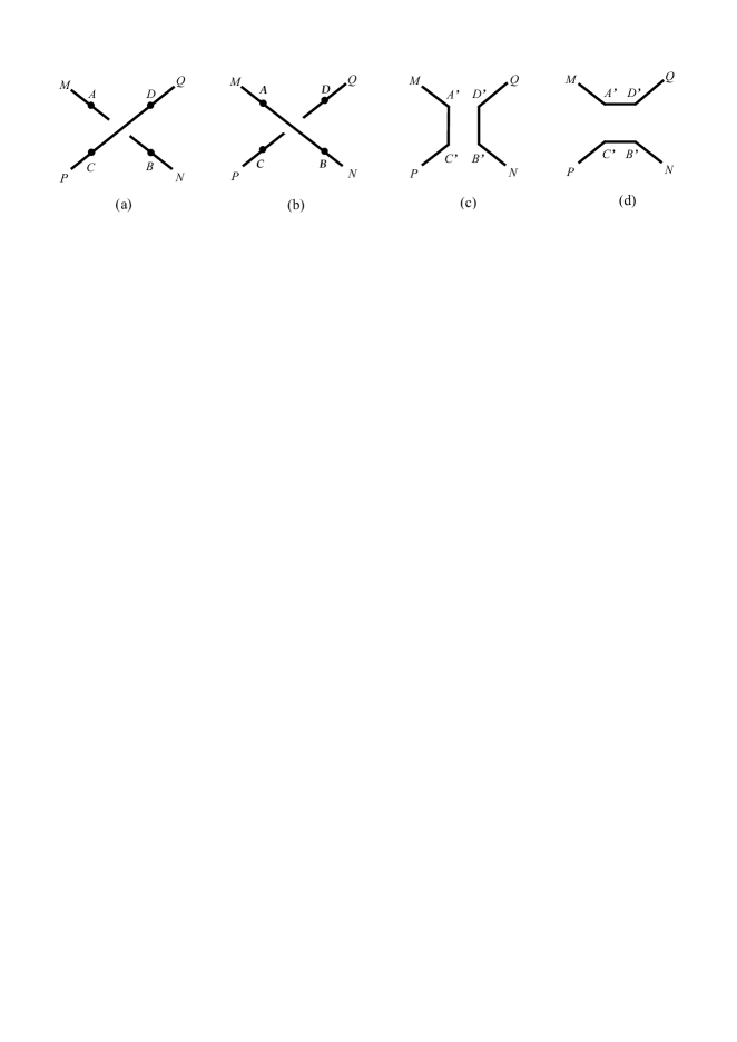
Figure 4: Crossing configurations of non-oriented knots: (a) over-crossing $L_{+}$; (b) under-crossing $L_{-}$; (c) non-crossing $L_{0}$; (d) non-crossing $L_{\infty}$.

Constructing

$$\left\langle\mathcal{L}\right\rangle\equiv t^{I\left(\mathcal{L}\right)},$$ (22)

our task is to show that $\left\langle\mathcal{L}\right\rangle$ satisfies (19) to (21). The first relation (19) is satisfied because $Tw\left(L_{c}\right)=0$ and thus $\left\langle L_{c}\right\rangle=t^{I\left(L_{c}\right)}=1$. For the second and third relations (20) and (21), their verifications will be detailed respectively in Subsections 3.1 and 3.2, where the evaluation of the constant $a$ is to be determined. Then, in Subsection 3.3, as an example the bracket polynomial for the right- and left-handed trefoil knots will be computed. In Subsection 3.4 the relationship between the Kauffman bracket polynomial and the Jones polynomial for oriented knots will be given.

3.1 Skein relation (20)

To realize (20) the relationships between $L_{\pm}$ and the $L_{0}$ and $L_{\infty}$ should be found. For this purpose, as before, we appeal to the trick “imaginarily adding paths”:

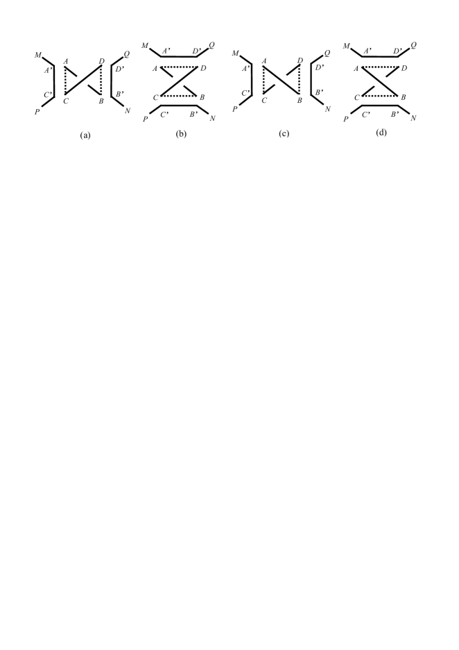
Figure 5: Imaginarily adding paths to $L_{+}$ and $L_{-}$: (a) $L_{0}$-type splitting of $L_{+}$; (b) $L_{\infty}$-type splitting of $L_{+}$; (c) $L_{0}$-type splitting of $L_{-}$; (d) $L_{\infty}$-type splitting of $L_{-}$.

• To relate $L_{+}$ to $L_{0}$, Figure 4(a) and 5(a) are considered. On the line $\overline{MN}$ of Figure 4(a), one breaks the point $A$ into a pair $\left(A,A^{\prime}\right)$, and breaks $B$ into $\left(B,B^{\prime}\right)$, as in Figure 5(a). On the line $\overline{PQ}$ of Figure 4(a), $C$ is broken into $\left(C,C^{\prime}\right)$ and $D$ into $\left(D,D^{\prime}\right)$ as in Figure 5(a). Thus $\overline{MN}$ turns to be $\overline{MA^{\prime}}\oplus\overline{AB}\oplus\overline{B^{\prime}N}$, and $\overline{PQ}$ to be $\overline{PC^{\prime}}\oplus\overline{CD}\oplus\overline{D^{\prime}Q}$. Introducing four imaginary segments $\overline{A^{\prime}C^{\prime}}$, $\overline{AC}$, $\overline{DB}$ and $\overline{D^{\prime}B^{\prime}}$ to Figure 5(a), the two sets $\left(\overline{MA^{\prime}},\overline{A^{\prime}C^{\prime}},\overline{C^{\prime}P}\right)$ and $\left(\overline{QD^{\prime}},\overline{D^{\prime}B^{\prime}},\overline{B^{\prime}N}\right)$ form an $L_{0}$ (i.e. $\overline{MA^{\prime}C^{\prime}P}\oplus\overline{QD^{\prime}B^{\prime}N}$), while the set $\left(\overline{AC},\overline{CD},\overline{DB},\overline{BA}\right)$ forms a writhe $\overline{ACDBA}$ which is the same as the $\gamma_{+}$ of Figure 3(a), disregarding orientations. Let this imaginarily constructed “$\gamma_{+}$” be denoted by $\widetilde{\gamma_{+}}$. These $L_{0}$ and $\widetilde{\gamma_{+}}$ are called an $L_{0}$-splitting of the $L_{+}$.
  Because all the knots we consider in this section are non-oriented, the added segments $\overline{A^{\prime}C^{\prime}}$, $\overline{D^{\prime}B^{\prime}}$, $\overline{AC}$ and $\overline{DB}$ should have no orientations either. Hence no path-cancellation may take place between these segments, different from what happened in the last section. The contributions of these segments to $t^{I\left(L_{+}\right)}$ should be discussed individually.
  Firstly, the $\overline{A^{\prime}C^{\prime}}$ and $\overline{D^{\prime}B^{\prime}}$ are trivial, because the $\overline{MA^{\prime}C^{\prime}P}\oplus\overline{QD^{\prime}B^{\prime}N}$ in Figure 5(a) does not contain the double point of $L_{+}$ and is a planar figure. So the segments $\overline{A^{\prime}C^{\prime}}$ and $\overline{D^{\prime}B^{\prime}}$ have no contribution to $\int_{\overline{MA^{\prime}C^{\prime}P}\oplus\overline{QD^{\prime}B^{\prime}N}}A_{i}dx^{i}$, and hence $\int_{\overline{MA^{\prime}}\oplus\overline{C^{\prime}P}\oplus\overline{QD^{\prime}}\oplus\overline{B^{\prime}N}}A_{i}dx^{i}$ $=\int_{\overline{MA^{\prime}C^{\prime}P}\oplus\overline{QD^{\prime}B^{\prime}N}}A_{i}dx^{i}=I\left(L_{0}\right)$.
  Secondly, in contrast, in Figure 5(a) the contributions of $\overline{AC}$ and $\overline{DB}$ are non-trivial. The $\widetilde{\gamma_{+}}$ contains the non-triviality of $L_{+}$ — the double point, hence as a stereoscopic figure it cannot be confined in two dimensions. Then the contributions of the realistic segments $\overline{CD}$ and $\overline{BA}$, $\int_{\overline{CD}\oplus\overline{BA}}A_{i}dx^{i}$, can only account for part of the integral over the whole $\widetilde{\gamma_{+}}:\int_{\overline{CD}\oplus\overline{BA}}A_{i}dx^{i}$ $=\lambda\oint\nolimits_{\widetilde{\gamma_{+}}}A_{i}dx^{i}$ $=\lambda I\left(\widetilde{\gamma_{+}}\right),$ where $\lambda$ is a formal ratio constant, $0<\lambda<1$. The $\lambda$ could be evaluated when compared to a concrete model. Since orientations of $\widetilde{\gamma_{+}}$ do not affect $\oint_{\widetilde{\gamma_{+}}}A_{i}dx^{i}$, the $t^{I\left(\widetilde{\gamma_{+}}\right)}$ is evaluated as the same as (11):

  $$t^{I\left(\widetilde{\gamma_{+}}\right)}=t^{\frac{1}{2}}.$$ (23)

  
  

  Thirdly, then, letting $t^{I\left(L_{+};L_{0}\mathrm{-splitting}\right)}$ be the contribution of $L_{0}$-splitting to $t^{I\left(\widetilde{\gamma_{+}}\right)}$, we have

  $$t^{I\left(L_{+};L_{0}\mathrm{-splitting}\right)}=t^{\lambda I\left(\widetilde{\gamma_{+}}\right)}t^{I\left(L_{0}\right)}=t^{\frac{\lambda}{2}}t^{I\left(L_{0}\right)}.$$ (24)

• Similarly, to relate $L_{+}$ to $L_{\infty}$ we consider Figure 4(a) and 5(b). Firstly, as in the above, the $\overline{MN}$ of Figure 4(a) turns to be $\overline{MA^{\prime}}\oplus\overline{AB}\oplus\overline{B^{\prime}N}$ of Figure 5(b), and $\overline{PQ}$ of 4(a) to be $\overline{PC^{\prime}}\oplus\overline{CD}\oplus\overline{D^{\prime}Q}$ of 5(b). Then introduce four imaginary segments $\overline{A^{\prime}D^{\prime}}$, $\overline{AD}$, $\overline{CB}$ and $\overline{C^{\prime}B^{\prime}}$ into Figure 5(b), to form an $L_{\infty}$ (i.e. $\overline{MA^{\prime}D^{\prime}Q}\oplus\overline{PC^{\prime}B^{\prime}N}$) and a $\widetilde{\gamma_{-}}$ (i.e. $\overline{ADCBA}$). This is called an $L_{\infty}$-splitting of the $L_{+}$.
  Secondly, as above, the $\overline{A^{\prime}D^{\prime}}$ and $\overline{C^{\prime}B^{\prime}}$ are trivial and therefore $\int_{\overline{MA^{\prime}}\oplus\overline{D^{\prime}Q}\oplus\overline{PC^{\prime}}\oplus\overline{B^{\prime}N}}A_{i}dx^{i}$ $=\int_{\overline{MA^{\prime}D^{\prime}Q}\oplus\overline{PC^{\prime}B^{\prime}N}}A_{i}dx^{i}$ $=I\left(L_{\infty}\right)$. The $\overline{AD}$ and $\overline{CB}$ are non-trivial and hence $\int_{\overline{CD}\oplus\overline{BA}}A_{i}dx^{i}$ $=\lambda\int_{\widetilde{\gamma_{-}}}A_{i}dx^{i}$ $=\lambda I\left(\widetilde{\gamma_{-}}\right)$ $=-\lambda I\left(\widetilde{\gamma_{+}}\right)$, where the ratio constant keeps to be $\lambda$ because $\widetilde{\gamma_{+}}$ and $\widetilde{\gamma_{-}}$ are mirror-symmetric.
  Thirdly, letting $t^{I\left(L_{+};L_{\infty}\mathrm{-splitting}\right)}$ be the contribution of $L_{\infty}$-splitting to $t^{I\left(L_{+}\right)}$, we have

  $$t^{I\left(L_{+};L_{\infty}\mathrm{-splitting}\right)}=t^{\lambda I\left(\widetilde{\gamma_{-}}\right)}t^{I\left(L_{\infty}\right)}=t^{-\lambda I\left(\widetilde{\gamma_{+}}\right)}t^{I\left(L_{\infty}\right)}.$$ (25)

• We deem that the $L_{+}$ represents an interaction between the two lines $\overline{MN}$ and $\overline{PQ}$ of Figure 4(a), and the $L_{0}$- and $L_{\infty}$-splitting are two channels to run this interaction. Therefore $t^{I\left(L_{+}\right)}$ is expressed as

  $$t^{I\left(L_{+}\right)}=t^{I\left(L_{+};L_{0}\mathrm{-splitting}\right)}+t^{I\left(L_{+};L_{\infty}\mathrm{-splitting}\right)}=t^{\lambda I\left(\widetilde{\gamma_{+}}\right)}t^{I\left(L_{0}\right)}+t^{-\lambda I\left(\widetilde{\gamma_{+}}\right)}t^{I\left(L_{\infty}\right)}.$$ (26)

  Introducing a constant $a$ as

  $$a\equiv t^{\lambda I\left(\widetilde{\gamma_{+}}\right)}=t^{\frac{\lambda}{2}},\ \ \ \mathrm{i.e.,}\ \ a^{-1}\equiv t^{\lambda I\left(\widetilde{\gamma_{-}}\right)}=t^{-\frac{\lambda}{2}},$$ (27)

  (26) is re-written as $\left\langle L_{+}\right\rangle=a\left\langle L_{0}\right\rangle+a^{-1}\left\langle L_{\infty}\right\rangle$, which is the desired first formula of (20).

Similarly, to relate $L_{-}$ to $L_{0}$ and $L_{\infty}$, we consider Figure 4(b), 5(c) and 5(d). Firstly, the $\overline{MN}$ of 4(b) turns to be the $\overline{MA^{\prime}}\oplus\overline{AB}\oplus\overline{B^{\prime}N}$ of Figure 5(c) or 5(d), and $\overline{PQ}$ of 4(b) to be $\overline{PC^{\prime}}\oplus\overline{CD}\oplus\overline{D^{\prime}Q}$ of 5(c) or 5(d). Then one introduces $\overline{A^{\prime}C^{\prime}}$, $\overline{AC}$, $\overline{DB}$ and $\overline{D^{\prime}B^{\prime}}$ in 5(c) to realize an $L_{0}$-splitting of $L_{-}$, and introduces $\overline{A^{\prime}D^{\prime}}$, $\overline{AD}$, $\overline{CB}$ and $\overline{C^{\prime}B^{\prime}}$ in 5(d) to realize an $L_{\infty}$-splitting of $L_{-}$. Secondly, using a similar analysis for $L_{+}$, we obtain for $L_{-}$ that

$$t^{I\left(L_{-};L_{0}\mathrm{-splitting}\right)}=t^{\lambda I\left(\widetilde{\gamma_{-}}\right)}t^{I\left(L_{0}\right)},\ \ \ \ \ \ t^{I\left(L_{-};L_{\infty}\mathrm{-splitting}\right)}=t^{\lambda I\left(\widetilde{\gamma_{+}}\right)}t^{I\left(L_{\infty}\right)}.$$ (28)

Hence

$$t^{I\left(L_{-}\right)}=t^{I\left(L_{-};L_{0}\mathrm{-splitting}\right)}+t^{I\left(L_{-};L_{\infty}\mathrm{-splitting}\right)}=t^{-\lambda I\left(\widetilde{\gamma_{+}}\right)}t^{I\left(L_{0}\right)}+t^{\lambda I\left(\widetilde{\gamma_{+}}\right)}t^{I\left(L_{\infty}\right)}.$$ (29)

In terms of the constant $a$ we arrive at the second formula of (20): $\left\langle L_{-}\right\rangle=a^{-1}\left\langle L_{0}\right\rangle+a\left\langle L_{\infty}\right\rangle$. This completes our verification of the second skein relation (20) of the Kauffman bracket polynomial.

3.2 Skein relation (21)

The third skein relation (21) is concerned with a union of two separate realistic components within a link.

Our starting point is to check the following fact for $\left\langle L_{c}\sqcup L\right\rangle:$

$$\left\langle L_{c}\sqcup L\right\rangle=a^{-1}\hat{L}_{+}+a\hat{L}_{-},$$ (30)

where $L_{c}$ is a trivial circle and $L$ an arbitrary link. $\hat{L}_{+}$ comes from adding a degree $\epsilon=+1$ writhe to $L$, as shown in Figure 6(a), and $\hat{L}_{-}$ from adding an $\epsilon=-1$ writhe to $L$, as shown in Figure 6(b).

Figure 6: Imaginarily adding $\widetilde{\gamma_{+}^{\prime\prime}}$ or $\widetilde{\gamma_{-}^{\prime\prime}}$ to the $L_{c}\sqcup L$: (a) $\hat{L}_{+}$; (b) $\hat{L}_{-}$; (c) $L_{c}\sqcup L$ with an added $\widetilde{\gamma_{+}^{\prime\prime}}$; (d) $L_{c}\sqcup L$ with an added $\widetilde{\gamma_{-}^{\prime\prime}}$.

The thought of the last subsection is instructive here for obtaining (30):

• To relate $\left\langle L_{c}\sqcup L\right\rangle$ to $\hat{L}_{+}$ we consider Figure 6(c), where an imaginary $\widetilde{\gamma_{+}^{\phantom{.}\prime\prime}}$ of Figure 3(c) without orientation is inserted into $\left\langle L_{c}\sqcup L\right\rangle$. The $\widetilde{\gamma_{+}^{\phantom{.}\prime\prime}}$ contains two realistic segments, $\overline{AB}$ and $\overline{CD}$, and two imaginary segments, $\overline{AC}$ and $\overline{DB}$. With respect to (24), such a $\widetilde{\gamma_{+}^{\phantom{.}\prime\prime}}$ has $\int_{\widetilde{\gamma_{+}^{\phantom{.}\prime\prime}}}A_{i}dx^{i}=a$. Then, choosing a trivial segment denoted by $\overline{A^{\prime}C^{\prime}}$ in the circle $L_{c}$, and a trivial $\overline{D^{\prime}B^{\prime}}$ in the link $L$, we obtain the union

  $$\hat{L}_{+}=\left(L_{c}\sqcup L\right)\oplus\widetilde{\gamma_{+}^{\phantom{.}\prime\prime}},$$ (31)

  which leads to

  $$L_{c}\sqcup L=\hat{L}_{+}\ominus\widetilde{\gamma_{+}^{\phantom{.}\prime\prime}},$$ (32)

  where $\ominus$ is the inverse operation of $\oplus$. This is called an $\hat{L}_{+}$-insertion of $L_{c}\sqcup L$. Thus, letting $t^{I\left(L_{c}\sqcup L;\hat{L}_{+}\mathrm{-insertion}\right)}$ be the contribution of $\hat{L}_{+}$-insertion to $t^{I\left(L_{c}\sqcup L\right)}$, one has

  $$t^{I\left(L_{c}\sqcup L;\hat{L}_{+}\mathrm{-insertion}\right)}=t^{I\left(\hat{L}_{+}\ominus\widetilde{\gamma_{+}^{\phantom{.}\prime\prime}}\right)}=t^{-I\left(\widetilde{\gamma_{+}^{\phantom{.}\prime\prime}}\right)}t^{I\left(\hat{L}_{+}\right)}=a^{-1}\left\langle\hat{L}_{+}\right\rangle,$$ (33)

  where the sign “$-$” in (33) arises from the operation “$\ominus$”.

• Similarly, to relate $\left\langle L_{c}\sqcup L\right\rangle$ to $\hat{L}_{-}$ we consider Figure 6(d), where a $\widetilde{\gamma_{-}^{\phantom{.}\prime\prime}}$ of Figure 3(d) is inserted into $\left\langle L_{c}\sqcup L\right\rangle$. The $\widetilde{\gamma_{-}^{\phantom{.}\prime\prime}}$ containing realistic $\overline{AB}$ and $\overline{CD}$ and imaginary $\overline{AC}$ and $\overline{DB}$ has $\int_{\widetilde{\gamma_{-}^{\phantom{.}\prime\prime}}}A_{i}dx^{i}=-a$. Then one has the union

  $$\hat{L}_{-}=\left(L_{c}\sqcup L\right)\oplus\widetilde{\gamma_{-}^{\phantom{.}\prime\prime}},$$ (34)

  and thus

  $$L_{c}\sqcup L=\hat{L}_{-}\ominus\widetilde{\gamma_{-}^{\phantom{.}\prime\prime}}.$$ (35)

  This is called an $\hat{L}_{-}$-insertion of $L_{c}\sqcup L$. Then, letting $t^{I\left(L_{c}\sqcup L;\hat{L}_{-}\mathrm{-insertion}\right)}$ be the contribution of $\hat{L}_{-}$-insertion to $t^{I\left(L_{c}\sqcup L\right)}$, one has

  $$t^{I\left(L_{c}\sqcup L;\hat{L}_{-}\mathrm{-insertion}\right)}=t^{I\left(\hat{L}_{-}\ominus\widetilde{\gamma_{-}^{\phantom{.}\prime\prime}}\right)}=t^{-I\left(\widetilde{\gamma_{-}^{\phantom{.}\prime\prime}}\right)}t^{I\left(\hat{L}_{-}\right)}=a\left\langle\hat{L}_{-}\right\rangle.$$ (36)

• We deem that in Figure 6(a) at the double point occurs the self-interaction of the vortex line $\hat{L}_{+}$, which has $\left(L_{c}\sqcup L\right)$ as one of its interaction channels. Similarly, in Figure 6(b) there occurs the self-interaction of $\hat{L}_{-}$ which has $\left(L_{c}\sqcup L\right)$ as an interaction channel. These imply $\left\langle L_{c}\sqcup L\right\rangle$ receives contributions from both Figure 6(a) and 6(b):

  $$\left\langle L_{c}\sqcup L\right\rangle=t^{I\left(L_{c}\sqcup L;\hat{L}_{+}\mathrm{-insertion}\right)}+t^{I\left(L_{c}\sqcup L;\hat{L}_{-}\mathrm{-insertion}\right)}=a^{-1}\left\langle\hat{L}_{+}\right\rangle+a\left\langle\hat{L}_{-}\right\rangle.$$ (37)

  (37) gives the required expression (30) for $\left\langle L_{c}\sqcup L\right\rangle$.

Then, on the other hand, according to the skein relation (20), $\left\langle\hat{L}_{+}\right\rangle$ and $\left\langle\hat{L}_{-}\right\rangle$ can also be obtained from $\left\langle L_{+}\right\rangle$ and $\left\langle L_{-}\right\rangle$ as

$$\left\langle\hat{L}_{+}\right\rangle=a\left\langle L_{c}\sqcup L\right\rangle+a^{-1}\left\langle L\right\rangle,\ \ \ \ \ \ \ \ \ \ \ \left\langle\hat{L}_{-}\right\rangle=a^{-1}\left\langle L_{c}\sqcup L\right\rangle+a\left\langle L\right\rangle.$$ (38)

Thus substituting (38) into (37) we precisely acquire

$$\left\langle L_{c}\sqcup L\right\rangle=-\left(a^{2}+a^{-2}\right)\left\langle L\right\rangle.$$ (39)

(39) gives the third skein relation (21) of the Kauffman bracket polynomial. We address that the sign “$-$” in the RHS of (39) should be understood as a consequence of the above algebraic deduction of (39).

A point should be stressed. The Kauffman bracket polynomial of a single loop $\gamma_{+}$ is $\left(-a^{3}\right)$, obtained from splitting the double point of $\gamma_{+}$ and using the skein relations (20) and (21). It is incorrect to directly use (23) to evaluate $\left\langle\gamma_{+}\right\rangle=t^{I\left(\widetilde{\gamma_{+}}\right)}=a$, because in the context of (23) the $\widetilde{\gamma_{+}}$ is an imaginary writhe rather than a realistic component. Similarly, for a single $\gamma_{-}$ its bracket polynomial reads $\left(-a^{-3}\right)$.

3.3 Example: trefoil knot

As an example, let us compute the Kauffman bracket polynomial of a right-handed trefoil knot in Figure 7 in the light of the skein relations (19) to (21).

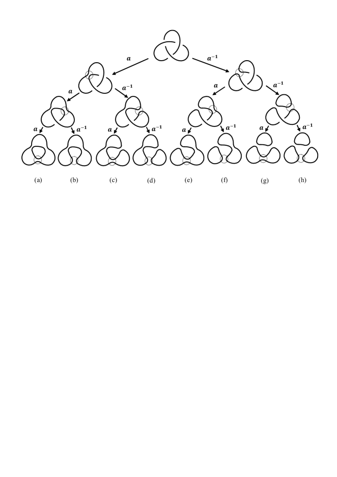
Figure 7: Computation of the Kauffman bracket polynomial of a right-handed trefoil knot. Top row: the right-handed trefoil knot. Bottom row: (a) – (h) are the eight statuses obtained after splitting the three double points of the trefoil knot.

Observe the three double points of the trefoil knot. Without loss of generality we regard each double point as an “$L_{+}$”-crossing, then the point has two kinds of splitting, the $L_{0}$- and $L_{\infty}$-splitting, which respectively contribute an “$a$” and an “$a^{-1}$” to the $\left\langle L_{+}\right\rangle$, according to (20). Thus, splitting the three double points one by one, as shown in Figure 7, we arrive at the eight completely-split figures shown in Figure 7(a) – 7(h). Each figure is called a status. Their respective polynomials are computed as follows:

• Status 7(a) comes from the original trefoil knot through three $L_{0}$-splittings which contribute $a^{3}$, according to (20); Status 7(a) contains two separate trivial circles which contribute one $\left(-a^{2}-a^{-2}\right)$, according to (21) and (19). Therefore the bracket polynomial of Status 7(a) reads: $-a^{3}\left(a^{2}+a^{-2}\right)$.

• Status 7(b) comes through two $L_{0}$-splittings and one $L_{\infty}$-splitting which totally contribute $a^{2}a^{-1}=a$, according to (20); Status 7(b) contains one circle which contributes a $1$, according to (19). Therefore the polynomial of Status 7(b) reads: $a$.

• Similarly, the polynomials of Status 7(c) to 7(h) read:

  7(c): $$a;$$ 7(d)

  7(e): 7(f):

  7(g): 7(h):

Hence the Kauffman bracket polynomial of the trefoil knot of Figure 7 is the sum of the polynomials of Status 7(a) – 7(h):

$$\left\langle\mathrm{Right\ handed\ trefoil\ knot}\right\rangle=-a^{5}-a^{-3}+a^{-7}.$$ (40)

Similarly, for a left-handed trefoil knot — the mirror image of the right-handed trefoil knot, obtained by changing the crossing situation of each double point to its inverse crossing — its bracket polynomial reads: $-a^{-5}-a^{3}+a^{7}$.

For a generic link $\mathcal{L}$ its Kauffman bracket polynomial can be similarly obtained by using the above status model. The result is

$$\left\langle\mathcal{L}\right\rangle=\sum_{s}a^{\theta_{0}\left(s\right)}a^{-\theta_{\infty}\left(s\right)}\left[\left(-a^{2}-a^{-2}\right)^{\left|s\right|-1}\right],$$ (41)

where all the double points of $\mathcal{L}$ have been split and $s$ denotes one of the statuses. $\theta_{0}\left(s\right)$ refers to the number of $L_{0}$-splittings during the splitting procedure of $\mathcal{L}$ towards obtaining Status $s$, and $\theta_{\infty}\left(s\right)$ refers to the number of $L_{\infty}$-splittings during the procedure towards obtaining $s$. The $\left|s\right|$ denotes the number of components (namely separate trivial circles) appearing in Status $s$.

3.4 Jones polynomial

The Jones polynomial for oriented links can be constructed from the Kauffman bracket polynomial [17].

The Jones polynomial is ambient isotopic, namely, it is invariant under all the three types of Reidemeister moves shown in Figure 8.

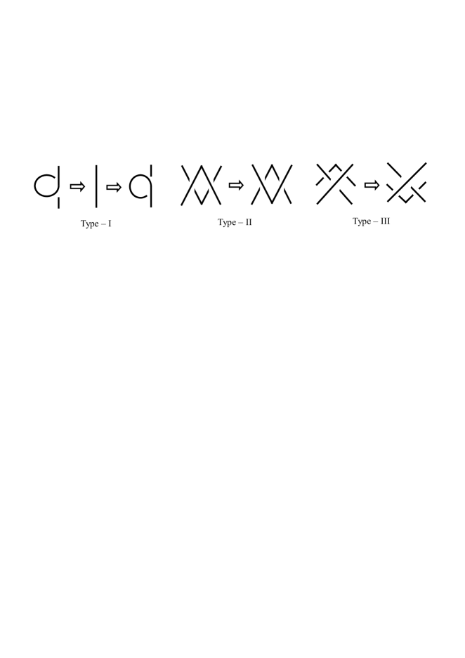
Figure 8: Three types of Reidemeister moves.

However, the Kauffman bracket polynomial is regularly isotopic, i.e., it is invariant only under type-II and -III Reidemeister moves, because the difference between $\left\langle\hat{L}_{\pm}\right\rangle$ and $\left\langle\hat{L}\right\rangle$ can be found with respect to (20) and (21):

$$\left\langle\hat{L}_{+}\right\rangle=-a^{3}\left\langle\hat{L}\right\rangle,\ \ \ \ \ \ \left\langle\hat{L}_{-}\right\rangle=-a^{-3}\left\langle\hat{L}\right\rangle,$$ (42)

which says the Kauffman bracket polynomial is not invariant under type-I Reidemeister moves. Therefore, in order to construct the Jones polynomial from the Kauffman bracket polynomial, one should not only endow knots with orientations, but also modify the bracket polynomial to be invariant under type-I moves.

From the algebraically topological point of view, the difference between $\left\langle\hat{L}_{\pm}\right\rangle$ and $\left\langle\hat{L}\right\rangle$ is given by

$$\left\langle\hat{L}_{+}\right\rangle=\alpha\left\langle\hat{L}\right\rangle,\ \ \ \ \ \ \left\langle\hat{L}_{-}\right\rangle=\alpha^{-1}\left\langle\hat{L}\right\rangle,$$ (43)

where $\alpha$ is a constant caused by adding a degree $\epsilon=1$ writhe to a link, and $\alpha^{-1}$ corresponds to the addition of an $\epsilon=-1$ writhe. Comparing (42) and (43) one obtains that $\alpha=-a^{3}$. Then, a new polynomial $V\left(\widehat{\mathcal{L}}\right)$ of $\widehat{\mathcal{L}}$ can be constructed from the Kauffman bracket polynomial $\left\langle\mathcal{L}\right\rangle$ by compensating the impact of $\alpha$:

$$V\left(\widehat{\mathcal{L}}\right)\equiv\alpha^{-w\left(\mathcal{L}\right)}\left\langle\mathcal{L}\right\rangle,$$ (44)

where $\widehat{\mathcal{L}}$ is an oriented link obtained by endowing a non-oriented link $\mathcal{L}$ with orientations. The $w\left(\mathcal{L}\right)$, called the algebraic writhing number of the link $\mathcal{L}$, is defined as $w\left(\mathcal{L}\right)\equiv\sum_{p}\epsilon\left(p\right)$, where $p$ denotes all the double points of $\mathcal{L}$, and $\epsilon\left(p\right)$ the degree of the point $p$. Now it can be checked that $V\left(\widehat{\mathcal{L}}\right)$ is an ambient isotopic polynomial

$$V\left(\widehat{\hat{L}_{\pm}}\right)=V\left(\widehat{\hat{L}}\right),$$ (45)

where $w\left(\hat{L}_{\pm}\right)=w\left(\hat{L}\right)\pm 1$ applies.

Eliminating $\left\langle L_{\infty}\right\rangle$ from the two formulae of (20), one has $a\left\langle L_{+}\right\rangle-a^{-1}\left\langle L_{-}\right\rangle=\left(a^{2}-a^{-2}\right)\left\langle L_{0}\right\rangle$. Replacing $\left\langle L_{+,-,0}\right\rangle$ with $V\left(\widehat{L_{+,-,0}}\right)$ and noticing $w\left(L_{\pm}\right)=w\left(L_{0}\right)\pm 1$, one obtains

$$a^{4}V\left(\widehat{L_{+}}\right)-a^{-4}V\left(\widehat{L_{-}}\right)=\left(a^{-2}-a^{2}\right)V\left(\widehat{L_{0}}\right).$$ (46)

Then, introducing a constant $\tau=a^{-4}$ for (46), and explicitly writing out (19), we acquire

$$V\left(L_{c}\right)=1$$ (47)

$$\tau^{-1}V\left(\widehat{L_{+}}\right)-\tau V\left(\widehat{L_{-}}\right)=\left(\tau^{\frac{1}{2}}-\tau^{-\frac{1}{2}}\right)V\left(\widehat{L_{0}}\right).$$ (48)

Eqs.(47) and (48) are recognized to be the well-known skein relations of the Jones polynomial. Hence $V\left(\widehat{\mathcal{L}}\right)$ is the desired Jones polynomial for oriented links.

4 Conclusion and discussion

In this paper we attempted to establish a direct relationship between the abelian CS action and link polynomial invariants of knot theory. We constructed a topological invariant $t^{I\left(\mathcal{L}\right)}$ for a link $\mathcal{L}$. In Section 2 it was shown that for oriented knotted vortex lines, $t^{I}$ satisfies the skein relations of the Kauffman R-polynomial. In Section 3 it was shown that for un-oriented knotted lines, $t^{I}$ satisfies the skein relations of the Kauffman bracket polynomial. As an example the bracket polynomials of the right- and left-handed trefoil knots were computed, and the Jones polynomial was constructed from the bracket polynomial. Our emphasis was placed on Section 3.

A point may be discussed. In Section 1 it was pointed out that the CS action $I$ can be expressed as $I=\sum_{k}\oint\nolimits_{\xi_{k}}A_{i}dx^{i}$ and the gauge potential $A_{i}$ has a decomposition $A_{i}=\epsilon^{ab}n^{a}\partial_{i}n^{b}$. Noticing $n^{a}$ is ill-defined on vortex lines, the Chern-Simons action $I$ contains indeterminateness. Therefore the use of Eq.(6) indeed means choosing a gauge for $I$. One can expect that other different choices of gauge conditions may yield different integration result, and thus yield different polynomial invariants for knots.

5 Acknowledgment

The author is indebted to Prof. Ruibin Zhang for useful discussions on the Kauffman polynomials and constant help in research. This work was financially supported by the USYD Postdoctoral Fellowship of the University of Sydney, Australia.

References

- [1] Witten E.: Commun. Math. Phys. 121 (1989) 351.
- [2] Jones V.F.R.: Invent. Math. 72 (1983) 1; ibid.: Ann. Math. 126 (1987) 335.
- [3] Guadagnini, E., Martellini, M., Mintchev, M.: Nucl. Phys. B 330 (1990) 575.
- [4] Labastida, J.M.F.: Chern-Simons Gauge Theory: Ten Years After, in Trends in Theoretical Physics II, H. Falomir, R. Gamboa, F. Schaposnik, eds., American Institute of Physics, New York, 1999, CP 484 (1-41), available at: hep-th/9905057.
- [5] Le T.T.Q., Murukami J., Ohtsuki T.: Topology 37 (1998) 539.
- [6] Rozansky L., Witten E.: Sel. Math. 3 (1997) 401.
-
[7]
Thompson G.: Adv. Theor. Math. Phys. 5
(2002) 457;
Hitchin N., Sawon J.: Duke Math. J. 106 (2001) 599. -
[8]
Gaiotto D., Witten E.: Janus configurations,
Chern-Simons couplings, and the -angle in super Yang-Mills theory, arXiv: 0804.2907;
Kapustin A., Saulina N.: Chern-Simons-Rozansky-Witten topological field theory, arXiv: 0904.1447. - [9] Moffatt H.K.: J. Fluid Mech. 35 (1969) 117.
- [10] Arnol’d V., Khesin B.: Topological Methods in Hydrodynamics, Springer, Heidelberg, 1998.
-
[11]
Moffatt H.K., Ricca, R.L.: Proc. R. Soc.
Lond. A 439 (1992) 411;
Moffatt H.K.: Reflections on Magnetohydrodynamics, in Perspectives in Fluid Dynamics, Batchelor, Moffatt and Worster ed., Cambridge University Press, 2000. -
[12]
Duan Y.S., Liu X., Fu L.B.: Phys. Rev. D 67
(2003) 085022;
Duan, Y.S., Liu, X.: JHEP 02 (2004) 028; and references therein. - [13] Wu T.T., Yang C.N.: Phys. Rev. D 12 (1975) 3845; ibid.: Phys. Rev. D 14 (1975) 437.
- [14] Polyakov A.M.: Mod. Phys. Lett. A 3 (1988) 325.
- [15] Rolfsen D.: Knots and Links, Publish or Perish, BerkleyCA, 1976.
-
[16]
Kauffman L.H.: Knots and Physics, 2nd ed.,
World Scientific, Singapore, 2001;
Kauffman L.H.: Rep. Prog. Phys. 68 (2005) 2829. - [17] Kauffman L.H.: On Knots, Princeton University Press, 1987.