Variants of the LLL Algorithm in Digital Communications: Complexity Analysis and Fixed-Complexity Implementation

Abstract

The Lenstra-Lenstra-Lovász (LLL) algorithm is the most practical lattice reduction algorithm in digital communications. In this paper, several variants of the LLL algorithm with either lower theoretic complexity or fixed-complexity implementation are proposed and/or analyzed. Firstly, the $O(n^{4}\log n)$ theoretic average complexity of the standard LLL algorithm under the model of i.i.d. complex normal distribution is derived. Then, the use of effective LLL reduction for lattice decoding is presented, where size reduction is only performed for pairs of consecutive basis vectors. Its average complexity is shown to be $O(n^{3}\log n)$, which is an order lower than previously thought. To address the issue of variable complexity of standard LLL, two fixed-complexity approximations of LLL are proposed. One is fixed-complexity effective LLL, while the other is fixed-complexity LLL with deep insertion, which is closely related to the well known V-BLAST algorithm. Such fixed-complexity structures are much desirable in hardware implementation since they allow straightforward constant-throughput implementation.

I Introduction

Lattice pre/decoding for the linear multi-input multi-output (MIMO) channel is a problem of high relevance in single/multi-antenna, broadcast, cooperative and other multi-terminal communication systems [1, 2, 3, 4]. Maximum-likelihood (ML) decoding for a rectangular finite subset of a lattice can be realized efficiently by sphere decoding [2, 5], whose complexity can nonetheless grow prohibitively with dimension $n$ [6]. The decoding complexity is especially felt in coded systems, where the lattice dimension is larger [7]. Thus, we often have to resort to approximate solutions, which mostly fall into two main streams. One of them is to reduce the complexity of sphere decoding, notably by relaxation or pruning; the former applies lattice reduction pre-processing and searches the infinite lattice, while the latter only searches part of the tree by pruning some branches. Another stream is lattice reduction-aided decoding [10, 11], which was first proposed by Babai in [12], which in essence applies zero-forcing (ZF) or successive interference cancelation (SIC) on a reduced lattice. It is known that Lenstra, Lenstra and Lovász (LLL) reduction combined with ZF or SIC achieves full diversity in MIMO fading channels [13, 14] and that lattice-reduction-aided decoding has constant gap to (infinite) lattice decoding [15]. It was further shown in [16] that minimum mean square error (MMSE)-based lattice-reduction aided decoding can achieve the optimal diversity and multiplexing tradeoff. In [17], it was shown that Babai’s decoding using MMSE provides near-ML performance for small-size MIMO systems. More recent research further narrowed down the gap to ML decoding by means of sampling [18] and embedding [19].

As can be seen, lattice reduction plays a crucial role in MIMO decoding. The celebrated LLL algorithm [20] features polynomial complexity with respect to the dimension for any given lattice basis but may not be strong enough for some applications. In practice of cryptanalysis where the dimension of the lattice can be quite high, block Korkin-Zolotarev (KZ) reduction is popular. Meanwhile, LLL with deep insertions (LLL-deep) is a variant of LLL that extends swapping in standard LLL to nonconsecutive vectors, thus finding shorter lattice vectors than LLL [21]. Lately, it is found that LLL-deep might be more promising than block-KZ reduction in high dimensions [22] since it runs faster than the latter.

Lattices in digital communications are complex-valued in nature. Since the original LLL algorithm was proposed for real-valued lattices [20], a standard approach to dealing with complex lattices is to convert them into real lattices. Although the real LLL algorithm is well understood, this approach doubles the dimension and incurs more computations. There have been several attempts to extend LLL reduction to complex lattices [23, 24, 25, 26]. However, complex LLL reduction is less understood. While our recent work has shown that the complex LLL algorithm lowers the computational complexity by roughly 50% [26], a rigorous complexity analysis is yet to be developed. In this paper, we analyze the complexity of complex LLL and propose variants of the LLL algorithm with either lower theoretic complexity or a fixed-complexity implementation structure.

More precisely, we shall derive the theoretic average complexity $O(n^{4}\log n)$ of complex LLL, assuming that the entries of $\mathbf{B}$ are be i.i.d. standard normal, which is the typical MIMO channel model. For integral bases, it is well known that the LLL algorithm has complexity bound $O(n^{4}\log B)$, where $B$ is the maximum length of the column vectors of basis matrix $\mathbf{B}$ [20]. The complexity of the LLL algorithm for real or complex-valued bases is less known. To the best of our knowledge, [27] was the only work prior to ours [28] on the complexity analysis of the real-valued LLL algorithm for a probabilistic model. However, [27] assumed basis vectors drawn independently from the unit ball of $\mathbb{R}^{n}$, which does not hold in MIMO communications.

Then, we propose the use of a variant of the LLL algorithm—effective LLL reduction in lattice decoding. The term effective LLL reduction was coined in [29], and was proposed independently by a number of researchers including [30]. We will show the average complexity bound $O(n^{3}\log n)$ in MIMO, i.e., an order lower than that of the standard LLL algorithm. This is because a weaker version of LLL reduction without full size reduction is often sufficient for lattice decoding. Besides, it can easily be transformed to a standard LLL-reduced basis while retaining the $O(n^{3}\log n)$ bound.

A drawback of the traditional LLL algorithm in digital communications is its variable complexity. The worst-case complexity could be quite large (see [31] for a discussion of the worst-case complexity), and could limit the speed of decoding hardware. To overcome this drawback, we propose two fixed-complexity approximations of the LLL algorithm, which are based on the truncation of the parallel structures of the effective LLL and LLL-deep algorithms, respectively. When implemented in parallel, the proposed fixed-complexity algorithms allow for higher reduction speed than the sequential LLL algorithm.

In the study of fixed-complexity LLL, we discover an interesting relation between LLL and the celebrated vertical Bell-labs space-time (V-BLAST) algorithm [32]. V-BLAST is a technique commonly used in digital communications that sorts the columns of a matrix for the purpose of better detection performance. It is well known that V-BLAST sorting does not improve the diversity order in multi-input multi-output (MIMO) fading channels; therefore it is not thought to be powerful enough. In this paper, we will show that V-BLAST and LLL are in fact closely related. More precisely, we will show that if a basis is both sorted in a sense closely related to V-BLAST and size-reduced, then it is reduced in the sense of LLL-deep.

Relation to prior work: The average complexity of real-valued effective LLL in MIMO decoding was analyzed by the authors in [28]. Jaldén et al. [31] gave a similar analysis of complex-valued LLL using a different method, yet the bound in [31] is less tight. A fixed-complexity LLL algorithm was given in [33], while the fixed-complexity LLL-deep was proposed by the authors in [34]. The fixed-complexity LLL-deep will also help demystify the excellent performance of the so-called DOLLAR (double-sorted low-complexity lattice-reduced) detector in [35], which consists of a sorted QR decomposition, a size reduction, and a V-BLAST sorting. Both its strength and weakness will be revealed in this paper.

The rest of the paper is organized as follows. Section II gives a brief review of LLL and LLL-deep. In Section III, we present the complexity analysis of complex LLL in MIMO decoding. Effective LLL and its complexity analysis are given in Section IV. Section V is devoted to fixed-complexity structures of LLL. Concluding remarks are given in Section VI.

Notation: Matrices and column vectors are denoted by upper and lowercase boldface letters (unless otherwise stated), and the transpose, Hermitian transpose, inverse of a matrix $\mathbf{B}$ by $\mathbf{B}^{T}$, $\mathbf{B}^{H}$, $\mathbf{B}^{-1}$, respectively. The inner product in the complex Euclidean space between vectors $\mathbf{u}$ and $\mathbf{v}$ is defined as $\langle\mathbf{u},\mathbf{v}\rangle=\mathbf{u}^{H}\mathbf{v}$, and the Euclidean length $\|\mathbf{u}\|=\sqrt{\langle\mathbf{u},\mathbf{u}\rangle}$. $\Re(x)$ and $\Im(x)$ denote the real and imaginary part of $x$, respectively. $\lceil x\rfloor$ denotes rounding to the integer closest to $x$. If $x$ is a complex number, $\lceil x\rfloor$ rounds the real and imaginary parts separately. The big O notation $f(x)=O(g(x))$ means for sufficiently large $x$, $f(x)$ is bounded by a constant times $g(x)$ in absolute value.

II The LLL Algorithm

Consider lattices in the complex Euclidean space $\mathbb{C}^{n}$. A complex lattice is defined as the set of points $L=\{\mathbf{Bx}|\mathbf{x}\in\mathcal{G}^{n}\}$, where $\mathbf{B}\in\mathbb{C}^{n\times n}$ is referred to as the basis matrix, and $\mathcal{G}=\mathbb{Z}+j\mathbb{Z}$, $j=\sqrt{-1}$ is the set of Gaussian integers. For convenience, we only consider a square matrix $\mathbf{B}$ in this paper, while the extension to a tall matrix is straightforward. Aside from the interests in digital communications [25, 26] and coding [36], complex lattices have found applications in factoring polynomials over Gaussian integers [24].

A lattice $L$ can be generated by infinitely many bases, from which one would like to select one that is in some sense nice or reduced. In many applications, it is advantageous to have the basis vectors as short as possible. The LLL algorithm is a polynomial time algorithm that finds short vectors within an exponential approximation factor [20]. The complex LLL algorithm, which is a modification of its real counterpart, has been described in [23, 24, 25, 26]. The complex LLL algorithm works directly with complex basis $\mathbf{B}$ rather than converting it into the real equivalent. Although the cost for each complex arithmetic operation is higher than its real counterpart, the total number of operations required for complex LLL reduction is approximately half of that for real LLL [26].

II-A Gram-Schmidt (GS) orthogonalization (O), QR and Cholesky decompositions

For a matrix $\mathbf{B}=[\mathbf{b}_{1},...,\mathbf{b}_{n}]\in\mathbb{C}^{n\times n}$, the classic GSO is defined as follows [37]

$$\mathbf{\hat{b}}_{i}=\mathbf{b}_{i}-\sum_{j=1}^{i-1}{\mu_{i,j}\mathbf{\hat{b}}_{j}},\quad\text{for }i=1,...,n$$ (1)

where $\mu_{i,j}=\langle\mathbf{b}_{i},\mathbf{\hat{b}}_{j}\rangle/\|\mathbf{\hat{b}}_{j}\|^{2}$. In matrix notation, it can be written as $\mathbf{B}=\mathbf{\hat{B}}\mbox{\boldmath{$\mu$}}^{T}$, where $\mathbf{\hat{B}}=[\mathbf{\hat{b}}_{1},...,\mathbf{\hat{b}}_{n}]$, and $\mbox{\boldmath{$\mu$}}=[\mu_{i,j}]$ is a lower-triangular matrix with unit diagonal elements.

GSO is closely related to QR decomposition $\mathbf{B}=\mathbf{QR}$, where $\mathbf{Q}$ is an orthonormal matrix and $\mathbf{R}$ is an upper-triangular matrix with nonnegative diagonal elements. More precisely, one has the relations $\mu_{j,i}=r_{i,j}/r_{i,i}$ and $\mathbf{\hat{b}}_{i}=r_{i,i}\cdot\mathbf{q}_{i}$ where $\mathbf{q}_{i}$ is the $i$-th column of $\mathbf{Q}$. QR decomposition can be implemented in various ways such as GSO, Householder and Givens transformations [37].

The Cholesky decomposition $\mathbf{A}=\mathbf{R}^{H}\mathbf{R}$ computes the R factor of the QR decomposition from the Gram matrix $\mathbf{A}=\mathbf{B}^{H}\mathbf{B}$. Given the Gram matrix, the computational complexity of Cholesky decomposition is approximately $n^{3}/3$, which is lower than $2n^{3}$ of QR decomposition [37].

II-B LLL Reduction

Definition 1 (Complex LLL)

Let $\mathbf{B}=\mathbf{\hat{B}}\mbox{\boldmath{$\mu$}}^{T}$ be the GSO of a complex-valued basis ${\bf B}$. ${\bf B}$ is LLL-reduced if both of the following conditions are satisfied:

$$|\Re(\mu_{i,j})|\leq 1/2\text{ and }|\Im(\mu_{i,j})|\ \leq 1/2$$ (2)

for $1\leq j<i\leq n$, and

$$\|\mathbf{\hat{b}}_{i}\|^{2}\geq(\delta-|\mu_{i,i-1}|^{2})\|\mathbf{\hat{b}}_{i-1}\|^{2}$$ (3)

for $1<i\leq n$, where $1/2<\delta\leq 1$ is a factor selected to achieve a good quality-complexity tradeoff.

The first condition is the size-reduced condition, while the second is known as the Lovász condition. It follows from the Lovász condition (3) that for an LLL-reduced basis

$$\|\mathbf{\hat{b}}_{i}\|^{2}\geq(\delta-1/2)\|\mathbf{\hat{b}}_{i-1}\|^{2},$$ (4)

i.e., the lengths of GS vectors do not drop too much.

Let $\alpha=1/(\delta-1/2)$. A complex LLL-reduced basis satisfies [23, 24]:

$$\begin{split}||{\bf b}_{1}||&\leq\alpha^{(n-1)/4}\text{det}^{1/n}L,\\ ||{\bf b}_{1}||&\leq\alpha^{(n-1)/2}\lambda_{1},\\ \prod_{i=1}^{n}||{\bf b}_{i}||&\leq\alpha^{n(n-1)/4}\det L,\\ \end{split}$$ (5)

where $\lambda_{1}$ is the length of the shortest vector in $L$, and $\det{L}\triangleq\det\mathbf{B}$. These properties show in various senses that the vectors of a complex LLL-reduced basis are not too long. Analogous properties hold for real LLL, with $\alpha$ replaced with $\beta=1/(\delta-1/4)$ [20]. It is noteworthy that although the bounds (5) for complex LLL are in general weaker than the real-valued counterparts, the actual performances of complex and real LLL algorithms are very close, especially when $n$ is not too large.

A size-reduced basis can be obtained by reducing each vector individually. The vector $\mathbf{b}_{k}$ is size-reduced if $|\Re(\mu_{k,l})|\leq 1/2$ and $|\Im(\mu_{k,l})|\leq 1/2$ for all $l<k$. Algorithm 1 shows how $\mathbf{b}_{k}$ is size-reduced against $\mathbf{b}_{l}$ ($l<k$). To size-reduce $\mathbf{b}_{k}$, we call Algorithm 1 for $l=k-1$ down to 1. Size-reducing $\mathbf{b}_{k}$ does not affect the size reduction of the other vectors. Furthermore, it is not difficult to see that size reduction does not change the GS vectors.

Algorithm 2 describes the LLL algorithm (see [26] for the pseudo-code of complex LLL). It computes a reduced basis by performing size reduction and swapping in an iterative manner. If the Lovász condition (3) is violated, the basis vectors $\mathbf{b}_{k}$ and $\mathbf{b}_{k-1}$ are swapped; otherwise it carries out size reduction to satisfy (2). The algorithm is known to terminate in a finite number of iterations for any given input basis $\mathbf{B}$ and for $\delta\leq 1$ [20] (note that this is true even when $\delta=1$ [38, 39]). By an iteration we mean the operations within the “while” loop in Algorithm 2, which correspond to an increment or decrement of the variable $k$.

Algorithm 1  Pairwise Size Reduction

Input: Basis vectors $\mathbf{b}_{k}$ and $\mathbf{b}_{l}$ ($l<k$)
          GSO coefficient matrix $[\mu_{i,j}]$
Output: Basis vector $\mathbf{b}_{k}$ size-reduced against $\mathbf{b}_{l}$
            Updated GSO coefficient matrix $[\mu_{i,j}]$

  if $|\Re(\mu_{k,l})|\geq 1/2$ or $|\Im(\mu_{k,l})|\geq 1/2$ then

     ${\bf b}_{k}:={\bf b}_{k}-\lceil\mu_{k,l}\rfloor{\bf b}_{l}$

     for $j=1,2,...,l$ do

        $\mu_{k,j}:=\mu_{k,j}-\lceil\mu_{k,l}\rfloor\mu_{l,j}$

Algorithm 2  LLL Algorithm

Input: A basis $\mathbf{B}=[\mathbf{b}_{1},...\mathbf{b}_{n}]$
Output: The LLL-reduced basis

1:  compute GSO $\mathbf{B}=\mathbf{\hat{B}}[\mu_{i,j}]^{T}$

2:  $k:=2$

3:  while $k\leq n$ do

4:     size-reduce $\mathbf{b}_{k}$ against $\mathbf{b}_{k-1}$

5:     if $\|\mathbf{\hat{b}}_{k}+\mu_{k,k-1}\mathbf{\hat{b}}_{k-1}\|^{2}<\delta\|\mathbf{\hat{b}}_{k-1}\|^{2}$ then

6:        swap $\mathbf{b}_{k}$ and $\mathbf{b}_{k-1}$ and update GSO

7:        $k:=\max(k-1,2)$

8:     else

9:        for $l=k-2,k-3,...,1$ do

10:           size-reduce $\mathbf{b}_{k}$ against $\mathbf{b}_{l}$

11:        $k:=k+1$

Obviously, for real-valued basis matrix $\mathbf{B}$, Definition 1 and Algorithm 2 coincide with the standard real LLL algorithm. Some further relations between real and complex LLL are discussed in Appendix A.

Remark 1

The LLL algorithm can also operate on the Gram matrix [40]. To do this, one applies the Cholesky decomposition and updates the Gram matrix. Everything else remains pretty much the same.

II-C LLL-Deep

LLL-deep extends the swapping step to all vectors before $\mathbf{b}_{k}$, as shown in Algorithm 3. The standard LLL algorithm is restricted to $i=k-1$ in Line 5. LLL-deep can find shorter vectors. However, there are no proven bounds for LLL-deep other than those for standard LLL. The experimental complexity of LLL-deep is a few times as much as that of LLL, although the worst-case complexity is exponential. To limit the complexity, it is common to restrict the insertion within a window [21]. However, we will not consider this window in this paper.

Algorithm 3  LLL Algorithm with Deep Insertion

Input: A basis $\mathbf{B}=[\mathbf{b}_{1},...\mathbf{b}_{n}]$
Output: The LLL-deep-reduced basis

1:  compute GSO $\mathbf{B}=\mathbf{\hat{B}}[\mu_{i,j}]^{T}$

2:  $k:=2$

3:  while $k\leq n$ do

4:     size-reduce $\mathbf{b}_{k}$ against $\mathbf{b}_{k-1},...,\mathbf{b}_{2},\mathbf{b}_{1}$

5:     if $\exists i,1\leq i<k$ such that $\sum_{j=i}^{k}\mu_{k,j}^{2}\|\mathbf{\hat{b}}_{j}\|^{2}<\delta\|\mathbf{\hat{b}}_{i}\|^{2}$ then

6:        for the smallest such $i$, insert $\mathbf{b}_{k}$ before $\mathbf{b}_{i}$ and update GSO

7:        $k:=\max(i,2)$

8:     else

9:        $k:=k+1$

III Complexity Analysis of Complex LLL

In the previous work [26], it was only qualitatively argued that complex LLL approximately reduces the complexity by half, while a rigorous analysis was lacking. In this section, we complement the work in [26] by evaluating the computational complexity in terms of (complex-valued) floating-point operations (flops). The other operations such as looping and swapping are ignored. The complexity analysis consists of two steps. Firstly, we bound the average number of iterations. Secondly, we bound the number of flops of a single iteration.

III-A Average Number of Iterations

To analyze the number of iterations, we use a standard argument, where we consider the LLL potential [20]

$$\mathcal{D}=\prod_{i=1}^{n-1}{\|\mathbf{\hat{b}}_{i}\|^{2(n-i)}}.$$ (6)

Obviously, $\mathcal{D}$ only changes during the swapping step. This happens when

$$\|\mathbf{\hat{b}}_{k}\|^{2}<(\delta-|\mu_{k,k-1}|^{2})\|\mathbf{\hat{b}}_{k-1}\|^{2}$$ (7)

for some $k$. After swapping, $\mathbf{\hat{b}}_{k-1}$ is replaced by $\mathbf{\hat{b}}_{k}+\mu_{k,k-1}\mathbf{\hat{b}}_{k-1}$. Thus $\|\mathbf{\hat{b}}_{k-1}\|^{2}$ as well as $\mathcal{D}$ shrinks by a factor less than $\delta$.

The number $K$ of iterations is exactly the number of Lovász tests. Let $K^{+}$ and $K^{-}$ be the numbers of positive and negative tests, respectively. Obviously, $K=K^{+}+K^{-}$. Since $k$ is incremented in a positive test and decremented in a negative test, and since $k$ starts at 2 and ends at $n$, we must have $K^{+}\leq K^{-}+(n-1)$ (see also [27]). Thus it is sufficient to bound $K^{-}$.

Let $A=\max_{i}{\|\mathbf{\hat{b}}_{i}\|^{2}}$ and $a=\min_{i}{\|\mathbf{\hat{b}}_{i}\|^{2}}$. The initial value of $\mathcal{D}$ can be bounded from above by $A^{n(n-1)/2}$. To bound the number of iterations for a complex-valued basis, we invoke the following lemma [20, 27], which holds for complex LLL as well.

Lemma 1

During the execution of the LLL algorithm, the maximum $A$ is non-increasing while the minimum $a$ is non-decreasing.

In other words, the LLL algorithm tends to reduce the interval $[a,A]$ where the squared lengths of GS vectors reside. From Lemma 1, we obtain

$$K^{-}\leq\frac{n(n-1)}{2}\log\frac{A}{a}$$ (8)

where the logarithm is taken to the base $1/\delta$ (this will be the case throughout the paper).

Assuming that the basis vectors are i.i.d. in the unit ball of $\mathbb{R}^{n}$, Daude and Vallee showed that the mean of $K^{-}$ is upper-bounded by $O(n^{2}\log n)$ [27]. The analysis for the i.i.d. Gaussian model is similar. Yet, here we use the exact value of $\mathcal{D}_{0}$, which is the initial value of $\mathcal{D}$, to bound the average number of iterations. It leads to a better bound than using the maximum $A$ in (8). The lower bound on $\mathcal{D}$ is followed:

$$\mathcal{D}_{\text{lower}}=\frac{n(n-1)}{2}\log a\leq\mathcal{D}.$$

Accordingly, the mean of $K^{-}$ is bounded by

$$\begin{split}E[K^{-}]&\leq E\left[\log\frac{\mathcal{D}_{0}}{\mathcal{D}_{\text{lower}}}\right]\\ &=E\left[\log\mathcal{D}_{0}\right]-E\left[\log\mathcal{D}_{\text{lower}}\right]\\ &=E\left[\log\mathcal{D}_{0}\right]-\frac{n(n-1)}{2}\log E\left[\log a\right].\end{split}$$ (9)

We shall bound the two terms separately.

The QR decomposition of an i.i.d. complex normal random matrix has the following property: the squares of the diagonal elements $r_{i,i}$ of the matrix $\mathbf{R}$ are statistically independent $\chi^{2}$ random variables with $2(n-i+1)$ degrees of freedom [41]. Since $r^{2}_{i,i}=\|\mathbf{\hat{b}}_{i}\|^{2}$, we have

$$\begin{split}E\left[\log\mathcal{D}_{0}\right]&=\sum_{i=1}^{n-1}{(n-i)E\left[\log\|\mathbf{\hat{b}}_{i}\|^{2}\right]}\\ &\leq\sum_{i=1}^{n-1}{(n-i)\log E\left[\|\mathbf{\hat{b}}_{i}\|^{2}\right]}\\ &=\sum_{i=1}^{n-1}{(n-i)\log 2(n-i+1)}\\ &\leq\frac{n(n-1)}{2}\log 2n\\ \end{split}$$ (10)

where the first inequality follows from Jensen’s inequality $E[\log X]\leq\log E[X]$.

It remains to determine $E\left[\log a\right]$. The cumulative distribution function (cdf) $F_{a}(x)$ of the minimum $a$ can be written as

$$F_{a}(x)=1-\prod_{i=1}^{n}\left[1-F_{i}(x)\right]$$

where $F_{i}(x)$ denotes the cdf of a $\chi^{2}$ random variables with $2i$ degrees of freedom:

$$\begin{split}F_{i}(x)&=\int_{0}^{x}{\frac{1}{2^{i}\Gamma(i)}y^{i-1}e^{-y/2}dy},\quad x\geq 0\\ &=1-e^{-x}\sum_{m=0}^{i-1}{\frac{x^{m}}{m!}}.\end{split}$$ (11)

As $n$ tends to infinity, $F_{a}(x)$ approaches a limit cdf $\bar{F}_{a}(x)$ that is not a function of $n$. Since $a$ deceases with $n$, $E\left[\log a\right]$ is necessarily bounded from below by its limit:

$$E\left[\log a\right]\geq\int_{0}^{\infty}\log xd\bar{F}_{a}(x).$$ (12)

The convergence of $F_{a}(x)$ is demonstrated in Fig. 1.

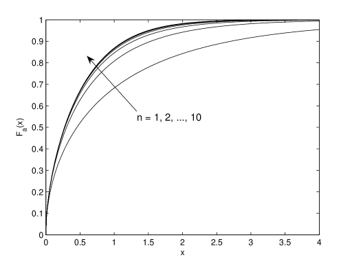
Figure 1: Convergence of $F_{a}(x)$ as $n$ increases.

Although it is difficult to evaluate the above integral exactly, we can derive a lower bound. To do this, we examine the behavior of the limit probability density function (pdf) $\bar{f}_{a}(x)$. $\bar{f}_{a}(x)$ is a decreasing function. Moreover, $\bar{f}_{a}(0)=1$. To show this, note that as $x\rightarrow 0^{+}$ we have the approximation $e^{-x}\approx 1-x$ and $\sum_{m=0}^{i-1}x^{m}/m!\approx 1+x$. Therefore, as $x\rightarrow 0^{+}$

$$\begin{split}\bar{F}_{a}(x)&\approx 1-\lim_{n\rightarrow\infty}(1-x)\prod_{i=2}^{n}{(1-x)(1+x)}\\ &=1-\lim_{n\rightarrow\infty}(1-x)(1-x^{2})^{n-1}\\ \end{split}$$ (13)

and accordingly $\bar{F}_{a}(x)\approx x$ as $x\rightarrow 0^{+}$. Then $\bar{f}_{a}(0)=d\bar{F}_{a}(x)/dx|_{x=0^{+}}=1$.

Then we have

$$\begin{split}E\left[\log a\right]&\geq\int_{0}^{\infty}\log x\bar{f}_{a}(x)dx\\ &\geq\int_{0}^{1}\log x\bar{f}_{a}(x)dx\\ &\geq\int_{0}^{1}\log xdx=-1\end{split}$$ (14)

where the last inequality follows from $\bar{f}(x)<1$ for $x>0$.

Substituting (10),(14) into (9), we obtain

$$E[K^{-}]\leq\frac{n(n-1)}{2}(\log 2n+1).$$ (15)

Therefore, we arrive at the following result:

Proposition 1

Under the i.i.d. complex normal model of the basis matrix $\mathbf{B}$, the total number of iterations of the LLL algorithm can be bounded as

$$E[K]\leq{n(n-1)}(\log 2n+1)+n\approx n^{2}\log n.$$ (16)

Remark 2

A similar analysis in [31] applied the bounds $\sigma_{1}\geq\sqrt{A}$ and $\sqrt{a}\geq\sigma_{n}$, where $\sigma_{1}$ and $\sigma_{n}$ are the maximum and minimum singular value of $\mathbf{B}$, respectively. Accordingly, the resultant bound $n^{2}\log(\sigma_{1}/\sigma_{n})$ is less tight. In fact, [31] showed the bound $E[K]\lesssim 4n^{2}\log n$, which is larger by a factor of 4.

III-B Number of Flops for Each Iteration

The second step proceeds as follows. Updating the GSO coefficients [20] during the swapping step costs $6(n-k)+7\leq 6n-5$ flops ($k\geq 2$), whereas pairwise size reduction for $(k,k-1)$ costs $2n+2(k-1)\leq 4n-2$ flops ($k\geq 2$). Testing the Lovász condition as (4) costs 3 flops each time. Besides, the initial GSO costs $2n^{3}$ flops. Therefore, excluding full size reduction, the cost is bounded by

$$\begin{split}\mathcal{C}_{1}&\leq(6n-5)K^{-}+(4n-2+3)(K^{-}+K^{+})+2n^{3}\\ &\leq(6n-5)\frac{n(n-1)}{2}\log 2n\\ &\quad+(4n+1)[n(n-1)\log 2n+(n-1)]+2n^{3}\\ &=7n^{2}(n-1)\log 2n-\frac{3}{2}n(n-1)\log 2n\\ &\quad+(4n+1)(n-1)+2n^{3}\\ &\leq 7n^{3}\log 2n+2n^{3}.\end{split}$$ (17)

During each step, the number of flops due to full size reduction is no more than

$${\sum_{l=1}^{k-2}{(2n+2l)}}\leq 3n^{2}.$$ (18)

Therefore, the subtotal amount of flops due to full size reduction are

$$\mathcal{C}_{2}=3n^{2}K^{+}\leq 3n^{2}\left[\frac{n(n-1)}{2}\log 2n+(n-1)\right]$$ (19)

which is $O(n^{4}\log n)$ and thus is dominant. This results in $O(n^{4}\log n)$ complexity bound on the overall complexity $\mathcal{C}=\mathcal{C}_{1}+\mathcal{C}_{1}$ of the complex LLL algorithm.

III-C Comparison with Real-valued LLL

In the conventional approach, the complex-valued matrix $\mathbf{B}$ is converted into real-valued $\mathbf{B}_{\text{R}}$ (see Appendix A). Obviously, $\mathbf{B}$ and $\mathbf{B}_{\text{R}}$ have the same values of $A$ and $a$, and same convergence speed determined by $\delta$. Since the size of $\mathbf{B}_{\text{R}}$ is twice that of $\mathbf{B}$, real LLL needs about four times as many iterations as complex LLL.

For real-valued LLL, the expressions (17) and (19) are almost the same [28], with a doubled size $n$. Under the assumption that on average a complex arithmetic operation costs four times as much as a real operation, $\mathcal{C}_{1}$ of complex LLL is half of that of real LLL. Meanwhile, when comparing $\mathcal{C}_{2}$, there is a subtle difference, i.e., the chance of full size reduction (Lines 9 and 10 in Algorithm 2) is doubled for complex LLL [26]. Therefore, $\mathcal{C}_{2}$ of complex LLL is also half. Then the total cost of complex LLL is approximately half.

III-D Reduction of the Dual Basis

Sometimes it might be more preferable to reduce the dual basis $\mathbf{B}^{*}\triangleq(\mathbf{B}^{-1})^{H}\mathbf{J}$, where $\mathbf{J}$ is the column-reversing matrix [15]. In the following, we show that the $O(n^{2}\log n)$ average number of iterations still holds.

Let $\mathbf{\hat{B}}^{*},A^{*},a^{*}$ be the corresponding notations for the dual basis. Due to the relation $\|\hat{\mathbf{b}}_{i}\|=\|\hat{\mathbf{b}}_{n-i+1}^{*}\|^{-1}$ [42], we have

$$\frac{A}{a}=\frac{1/a^{*}}{1/A^{*}}=\frac{A^{*}}{a^{*}}.$$

Thus, the bound on the number of iterations is exactly the same. In particular, the average number of iterations is the same.

In MIMO broadcast, it is $\mathbf{B}^{-1}$ that needs to be reduced [43]. Noting that $\mathbf{B}^{-1}$ has the same statistics as $(\mathbf{B}^{-1})^{H}\mathbf{J}$ because $\mathbf{B}$ is i.i.d. normal, it is easy to see that the bound on $K^{-}$ is again the same.

Remark 3

The same conclusion was drawn in [31] by examining the singular values.

IV Effective LLL Reduction

IV-A Effective LLL

Since some applications such as sphere decoding and SIC only require the GS vectors $\mathbf{\hat{b}}_{i}$ rather than the basis vectors themselves, and since size reduction does not change them, a weaker version of the LLL algorithm is sufficient for such applications. This makes it possible to devise a variant of the LLL algorithm that has lower theoretic complexity than the standard one.

From the above argument it seems that we would be able to remove the size reduction operations at all. However, this is not the case. An inspection shows that the size-reduced condition for two consecutive basis vectors

$$|\Re(\mu_{i,i-1})|\leq 1/2\text{ and }|\Im(\mu_{i,i-1})|\ \leq 1/2,\quad 1<i\leq n$$ (20)

is essential in maintaining the lengths of the GS vectors. In other words, (20) must be kept along with the Lovász condition so that the lengths of GS vectors will not be too short. Note that their lengths are related to the performance of SIC and the complexity of sphere decoding. We want the lengths to be as even as possible so as to improve the SIC performance and reduce the complexity of sphere decoding.

A basis satisfies condition (20) and the Lovász condition (3) is called an effectively LLL-reduced basis in [29]. Effective LLL reduction terminates in exactly the same number of iterations, because size-reducing against other vectors has no impact on the Lovász test. In addition to (4), an effectively LLL-reduced basis has other nice properties. For example, if a basis is effectively LLL-reduced, so is its dual basis [29, 24].

Effective LLL reduction permits us to remove from Algorithm 2 the most expensive part, i.e., size-reducing $\mathbf{b}_{k}$ against $\mathbf{b}_{k-2},\mathbf{b}_{k-3},...,\mathbf{b}_{1}$ (Lines 9-10). For integral bases, doing this may cause excessive growth of the (rational) GSO coefficients $\mu_{i,j}$, $j<i-1$, and the increase of bit lengths will likely offset the computational saving. This is nonetheless not a problem in MIMO decoding, since the basis vectors and GSO coefficients can be represented by floating-point numbers after all. We use a model where floating-point operations take constant time, and accuracy is assumed not to perish. There is strong evidence that this model is practical, because the correctness of floating-point LLL for integer lattices has been proven [40]. Although the extension of the proof to the case of continuous bases seems very difficult, in practice this model is valid as long as the arithmetic precision is sufficient for the lattice dimensions under consideration.

We emphasize that under this condition the effective and standard LLL algorithms have the same error performance in the application to SIC and sphere decoding, as asserted by Proposition 2.

Proposition 2

The SIC and sphere decoder with effective LLL reduction finds exactly the same lattice point as that with standard LLL reduction.

Proof:

This is obvious since SIC and sphere decoding only need the GS vectors and since standard and effective LLL give exactly the same GS vectors. ∎

IV-B Transformation to Standard LLL-Reduced Basis

On the other hand, ZF does require the condition of full size reduction. One can easily transform an effective LLL-reduced basis into a fully reduced one. To do so, we simply perform size reductions at the end to make the other coefficients $|\Re(\mu_{i,j})|\leq 1/2$ and $|\Im(\mu_{i,j})|\leq 1/2$, for $1\leq j<i-1$, $2<i\leq n$ [44, 24]. This is because, once again, such operations have no impact on the Lovász condition. Full size reduction costs $O(n^{3})$ arithmetic operations. The analysis in the following subsection will show the complexity of this version of LLL reduction is on the same order of that of effective LLL reduction. In other words, it has lower theoretic complexity than the standard LLL algorithm.

There are likely multiple bases of the lattice $L$ that are LLL-reduced. For example, a basis reduced in the sense of Korkin-Zolotarev (KZ) is also LLL-reduced. Proposition 3 shows that this version results in the same reduced basis as the LLL algorithm.

Proposition 3

Fully size-reducing an effectively LLL-reduced basis gives exactly the same basis as the standard LLL algorithm.

Proof:

It is sufficient to prove the GSO coefficient matrix $[\mu_{i,j}]$ is the same, since $\mathbf{B}=\mathbf{\hat{B}}[\mu_{i,j}]^{T}$ and since $\mathbf{\hat{B}}$ is not changed by size reduction. We prove it by induction. Suppose the new version has the same coefficients $\mu_{i,j}$, $j<i$ when $i=2,...,k-1$. Note that this is obviously true when $i=2$.

When $i=k$ and $l=k-2$, the new version makes $|\Re(\mu_{k,k-2})|<1/2$ and $|\Im(\mu_{k,k-2})|<1/2$ at the end by subtracting its integral part so that

$$|\Re(\mu_{k,k-2}-\lceil\mu_{k,k-2}\rfloor)|<1/2,\text{ }|\Im(\mu_{k,k-2}-\lceil\mu_{k,k-2}\rfloor)|<1/2.$$

The standard LLL algorithm achieves this in a number of iterations. Yet the sum of integers subtracted must be equal. The other coefficients will be updated as

$$\mu_{k,j}:=\mu_{k,j}-\lceil\mu_{k,k-2}\rfloor\mu_{k-2,j},\quad j=1,...,k-3,$$

which will remain the same since coefficients $\mu_{k-2,j}$ are assumed to be the same.

Clearly, the argument can be extended to the case $i=k$ and $l=k-3,\cdots,1$. That is, the new version also has the same coefficients $\mu_{k,j}$, $j<k$. This completes the proof. ∎

IV-C $O(n^{3}\log n)$ Complexity

Proposition 4

Under the i.i.d. complex normal model of the basis $\mathbf{B}$, the average complexity of effective LLL is bounded by $\mathcal{C}_{1}$ in (17) which is $O(n^{3}\log n)$.

Proof:

Since the number of iterations is the same, and since each iteration of effective LLL costs $O(n)$ arithmetic operations, the total computation cost is $O(n^{3}\log n)$. More precisely, the effective LLL consists of the following computations: initial GSO, updating the GSO coefficients during the swapping step, pairwise size reduction, and testing the Lovász condition. Therefore, the total cost is exactly bounded by $\mathcal{C}_{1}$ in (17). ∎

To obtain a fully reduced basis, we further run pairwise size reduction for $l=k-2$ down to 1 for each $k=3,\cdots,n$. The additional number of flops required is bounded by

$$\begin{split}\sum_{k=3}^{n}{\sum_{l=1}^{k-2}{(2n+2l)}}&=\sum_{k=3}^{n}{{[2n(k-2)+(k-1)(k-2)]}}\\ &=\frac{4}{3}n(n-1)(n-2)\leq\frac{4}{3}n^{3}.\end{split}$$ (21)

Obviously, the average complexity is still $O(n^{3}\log n)$.

Again, since each complex arithmetic operation on average requires four real arithmetic operations, the net saving in complexity due to complex effective LLL is about 50%.

In Fig. 2, we show the theoretic upper bounds and experimental results for effective and standard LLL algorithms. Clearly there is room to improve the analysis. This is because our work is in fact a blend of worst- and average-case analysis, and the resultant theoretic bound is unlikely to be sharp. But nonetheless, the experimental data exhibit cubic growth with $n$, thereby supporting the $O(n^{3}\log n)$ bound. On the other hand, surprisingly, the experimental complexity of standard LLL reduction is not much higher than that of effective LLL. We observed that this is because of the small probability to execute size reduction with respect to nonconsecutive vectors (Lines 9-10 of the standard LLL algorithm), which were thought to dominate the complexity.

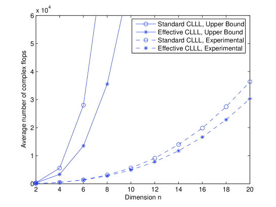
Figure 2: Average number of complex flops for effective CLLL reduction with $\delta=3/4$ for the i.i.d. normal basis model.

V Fixed-Complexity Implementation

Although the average complexity of the LLL algorithm is polynomial, it is important to recognize that its complexity is in fact variable due to its sequential nature. The worst-case complexity could be very large [31], which may severely limit the throughput of the decoder. In this Section, we propose two fixed-complexity structures that are suitable to approximately implement the LLL algorithm in hardware. One is fixed-complexity effective LLL, while the other is fixed-complexity LLL-deep. The structures are based on parallel versions of the LLL and LLL-deep algorithms, respectively. The parallel versions exhibit fast convergence, which allow to fix the number of iterations without incurring much quality degradation.

V-A Fixed-Complexity Effective LLL

Recently, a fixed-complexity LLL algorithm was proposed in [33]. It resembles the parallel ‘even-odd’ LLL algorithm earlier proposed in [45] (see also [46] for a systolic-array implementation) and a similar algorithm in [30]. It is well known that the LLL reduction can be achieved by performing size reduction and swapping in any order. Therefore, the idea in [33] was to run a super-iteration where the index $k$ is monotonically incremented from 2 to $n$, and repeat this super-iteration until the basis is reduced. This is slightly different from the ‘even-odd’ LLL [45], where the super-iteration is performed for even and odd indexes $k$ separately.

Here, we extend this fixed-complexity structure to effective LLL, which is a truncated version of the parallel effective LLL described in Algorithm 4 (one can easily imagine an ‘even-odd’ version of this algorithm). The index $k$ is never reduced in a super-iteration. Of course, one can further run full size reduction to make the basis reduced in the sense of LLL. It is easy to see that this algorithm converges by examining the LLL potential function. To cater for fixed-complexity implementation, we run a sufficiently large but fixed number of super-iterations.

How many super-iterations should we run? A crude estimate is $O(n^{2}\log n)$, i.e., the same as that for standard LLL. Since there is at least one swap within a super-iteration (otherwise the algorithm terminates), the number of super-iterations is bounded by $O(n^{2}\log n)$ (this is the approach used in [33]). However, this approach might be pessimistic, as up to $n-1$ swaps may occur in one super-iteration. Next, we shall argue that on average it is sufficient to run $O(n\log n)$ super-iterations in order to obtain a good basis. Accordingly, since each super-iteration costs $O(n^{2})$, the overall complexity is $O(n^{3}\log n)$.

Algorithm 4  Parallel Effective LLL Algorithm

Input: A basis $\mathbf{B}=[\mathbf{b}_{1},...\mathbf{b}_{n}]$
Output: Effectively LLL-reduced basis

1:  compute GSO $\mathbf{B}=\mathbf{\hat{B}}[\mu_{i,j}]^{T}$

2:  while any swap is possible do

3:     for $k=2,3,...,n$ do

4:        size-reduce $\mathbf{b}_{k}$ against $\mathbf{b}_{k-1}$

5:        if $\|\mathbf{\hat{b}}_{k}+\mu_{k,k-1}\mathbf{\hat{b}}_{k-1}\|^{2}<\delta\|\mathbf{\hat{b}}_{k-1}\|^{2}$ then

6:           swap $\mathbf{b}_{k}$ and $\mathbf{b}_{k-1}$ and update GSO

Proposition 5

Let $c=\frac{1}{\delta^{2}(\delta-\frac{1}{2})}$ for complex LLL and $c=\frac{1}{\delta^{2}(\delta-\frac{1}{4})}$ for real LLL. On average the fixed-complexity effective LLL finds a short vector with length

$$\|\mathbf{b}_{1}\|\leq\frac{c^{(n-1)/4}}{\sqrt{\delta}}\text{det}^{1/n}L$$ (22)

after $O(n\log n)$ super-iterations.

Proof:

The proof is an extension of the analysis of ‘even-odd’ LLL in [47], with two modifications.

Following [47], define the ratios

$$v(i)=\frac{\prod_{j=1}^{i}{\|\hat{\mathbf{b}}_{j}\|^{2}}}{c^{\frac{i(n-i)}{2}}(\det L)^{\frac{2i}{n}}}.$$ (23)

Let $v_{\text{max}}=\max{\{v(i),1\leq i\leq n\}}$. Following [47] one can prove that if $v_{\max}>\frac{1}{\delta}$ and $v(i)>\delta v_{\max}$, then the swapping condition is satisfied, i.e., $\|\hat{\mathbf{b}}_{i+1}\|^{2}\leq(\delta-|\mu_{i+1,i}|^{2})\|\hat{\mathbf{b}}_{i}\|^{2}$. Thus, after swapping, any such $v(i)$ will be decreased by a factor less than $\delta$; all other ratios do not increase. Hence $v_{\max}$ will be decreased by a factor less than $\delta$.

The first modification is bounding $v_{\max}$ in the beginning. We can see that in the beginning $v_{\max}\leq A^{n}/\text{det}^{2}L\leq(A/a)^{n}$ (recall $A=\max_{i=1}^{n}\|\hat{\mathbf{b}}_{i}\|^{2}$ and $a=\min_{i=1}^{n}\|\hat{\mathbf{b}}_{i}\|^{2}$).

Secondly, we need to check whether the swapping condition $\|\hat{\mathbf{b}}_{i+1}\|^{2}\leq(\delta-|\mu_{i+1,i}|^{2})\|\hat{\mathbf{b}}_{i}\|^{2}$ remains satisfied after $k$ goes from 2 to $i$. It turns out to be true. This is because $\|\hat{\mathbf{b}}_{i}\|^{2}$ will not decrease; in fact, the new $\|\hat{\mathbf{b}}_{i}\|^{2}$ increases by a factor larger than $1/\delta$ if ${\mathbf{b}}_{i-1}$ and ${\mathbf{b}}_{i}$ are swapped. Thus, ${\mathbf{b}}_{i}$ and ${\mathbf{b}}_{i+1}$ will always be swapped regardless of the swap between ${\mathbf{b}}_{i-1}$ and ${\mathbf{b}}_{i}$, and accordingly $v(i)$ will be decreased.

Thus, one has $v_{\max}\leq\frac{1}{\delta}$ after $O\left(n\log A-2\log(\det L)\right)\leq O(n\log A/a)$ iterations. On average this is $O(n\log n)$.

In particular, $v(1)\leq 1/\delta$ implies that $\mathbf{b}_{1}$ is short, with length bounded in (22). ∎

Remark 4

This analysis also applies to the fixed-complexity LLL proposed in [33] (this is obvious since size reduction does not change GSO).

Remark 5

Compared to (5) for standard sequential LLL, the approximation factor in (22) is larger by a coefficient $(\frac{1}{\delta})^{n/2}$. Yet we can make this factor very small by choosing $\delta\lessapprox 1$. For example, if $\delta=0.99$, then $(\frac{1}{\delta})^{n/2}<1.5$ for $n$ up to 80.

Remark 6

In practice, one can obtain a good basis after $n$ super-iterations. This will be confirmed by simulation later in this section.

Remark 7

Although we have only bounded the length of $\mathbf{b}_{1}$, this suffices for some applications in lattice decoding. For example, the embedding technique (a.k.a. augmented lattice reduction [19]) only requires a bound for the shortest vector.

V-A1 Relation to PMLLL

Another variant of the LLL algorithm, PMLLL, was proposed in [30], which repeats two steps: one is a series of swapping to satisfy the Lovász condition (even forgetting about $|\mu_{k,k-1}|\leq 1/2$), the other is size reduction to make $|\mu_{k,k-1}|\leq 1/2$ for $k=2,...,n$. This variant is similar to parallel effective LLL. However, $k$ does not necessarily scan from $2$ to $n$ monotonically in PMLLL.

V-B Fixed-Complexity LLL-Deep

Here, we propose another fixed-complexity structure to approximately implement LLL-deep (and, accordingly, LLL). More precisely, we apply sorted GSO and size reduction alternatively. This structure is closely related to V-BLAST.

The sorted GSO relies on the modified GSO [37]. At each step, the remaining columns of $\mathbf{B}$ are projected onto the orthogonal complement of the linear space spanned by the GS vectors already obtained. In sorted GSO, one picks the shortest GS vector at each step, which corresponds to the sorted QR decomposition proposed by Wubben et al [48] (we will use the terms sorted GSO and sorted QR decomposition interchangeably). Algorithm 5 describes the process of sorted GSO.

For $i=1,...,n$, let $\pi_{i}$ denote the projection onto the orthogonal complement of the subspace spanned by vectors $\mathbf{b}_{1},...,\mathbf{b}_{i-1}$. Then the sorted GSO has the following property: $\mathbf{b}_{1}$ is the shortest vector among $\mathbf{b}_{1}$, $\mathbf{b}_{2}$, …, $\mathbf{b}_{n}$; $\pi_{2}(\mathbf{b}_{2})$ is the shortest among $\pi_{2}(\mathbf{b}_{2})$, …, $\pi_{2}(\mathbf{b}_{n})$; and so on .

Sorted GSO tends to reduce $\max\{\|\mathbf{\hat{b}}_{1}\|,\|\mathbf{\hat{b}}_{2}\|,\cdots,\|\mathbf{\hat{b}}_{n}\|\}$. In fact, using proof by contradiction, we can show that sorted GSO minimizes $\max\{\|\mathbf{\hat{b}}_{1}\|,\|\mathbf{\hat{b}}_{2}\|,\cdots,\|\mathbf{\hat{b}}_{n}\|\}$. This is in contrast (but also very similar in another sense) to V-BLAST which maximizes $\min\{\|\mathbf{\hat{b}}_{1}\|,\|\mathbf{\hat{b}}_{2}\|,\cdots,\|\mathbf{\hat{b}}_{n}\|\}$ [32].

Algorithm 5  Sorted GSO

Input: A basis $\mathbf{B}=[\mathbf{b}_{1},...\mathbf{b}_{n}]$
Output: GSO for the sorted basis

1:  let $\mathbf{\hat{B}}=\mathbf{B}$

2:  for $i=1,2,...,n$ do

3:     $k=\arg\min_{i\leq m\leq n}{\|\mathbf{\hat{b}}_{m}\|}$

4:     exchange the $i$ and $k$-th columns of $\mathbf{\hat{B}}$

5:     for $j=i+1,...,n$ do

6:        compute the coefficient $\mu_{ij}=\frac{\langle\mathbf{\hat{b}}_{j},\mathbf{\hat{b}}_{i}\rangle}{\|\mathbf{\hat{b}}_{i}\|^{2}}$

7:        update $\mathbf{\hat{b}}_{j}:=\mathbf{\hat{b}}_{j}-\mu_{ij}\mathbf{\hat{b}}_{i}$

8:        %% joint sorted GSO and size reduction %%

9:        % $\mathbf{{b}}_{j}:=\mathbf{{b}}_{j}-\lceil\mu_{ij}\rfloor\mathbf{{b}}_{i}$

Following sorted GSO, it is natural to define the following notion of lattice reduction:

$$\begin{split}|\Re(\mu_{i,j})|&\leq 1/2,\quad|\Im(\mu_{i,j})|\ \leq 1/2,\quad\text{for}\quad 1\leq j<i\leq n;\\ \|\pi_{i}(\mathbf{b}_{i})\|&=\min\{\|\pi_{i}(\mathbf{b}_{i})\|,\|\pi_{i}(\mathbf{b}_{i+1})\|,...,\|\pi_{i}(\mathbf{b}_{n})\|\},\\ &\quad\text{for}\quad 1\leq i<n.\end{split}$$ (24)

In words, the basis is size-reduced and sorted in the sense of sorted GSO. Such a basis obviously exists, as a KZ-reduced basis satisfies the above two conditions [42]. In fact, KZ reduction searches for the shortest vector in the lattice with basis $[\pi_{i}(\mathbf{b}_{i})$, …, $\pi_{i}(\mathbf{b}_{n})]$.

The sorting condition is in fact stronger than the Lovász condition. Since $\mathbf{\hat{b}}_{i}+\mu_{i,i-1}\mathbf{\hat{b}}_{i-1}=\pi_{i-1}(\mathbf{b}_{i})$ and $\mathbf{\hat{b}}_{i-1}=\pi_{i-1}(\mathbf{b}_{i-1})$, the Lovász condition with $\delta=1$ turns out to be

$$\|\pi_{i-1}(\mathbf{b}_{i-1})\|\leq\|\pi_{i-1}(\mathbf{b}_{i})\|,\text{ for }1<i\leq n,$$ (25)

which can be rewritten as

$$\|\pi_{i}(\mathbf{b}_{i})\|=\min\{\|\pi_{i}(\mathbf{b}_{i})\|,\|\pi_{i}(\mathbf{b}_{i+1})\|\},\quad 1\leq i<n.$$ (26)

Obviously, this is weaker than the sorting condition for all Gram-Schmidt vectors. Therefore, the reduction notion defined above is stronger than LLL reduction even with $\delta=1$, but is weaker than KZ reduction.

Meanwhile, when LLL-deep terminates, the following condition is satisfied:

$$\delta\|\mathbf{\hat{b}}_{i}\|^{2}\leq\sum_{j=i}^{k}\mu_{k,j}^{2}\|\mathbf{\hat{b}}_{j}\|^{2}\quad\text{for }i<k\leq n.$$ (27)

If $\delta=1$, this is equivalent to $\|\pi_{i}(\mathbf{b}_{i})\|=\min\{\|\pi_{i}(\mathbf{b}_{i})\|,\|\pi_{i}(\mathbf{b}_{i+1})\|,...,\|\pi_{i}(\mathbf{b}_{n})\|\}$. Therefore, we have

Proposition 6

The notion of lattice reduction defined in (24) is equivalent to LLL-deep with $\delta=1$ and unbounded window size.

Although this notion is the same as LLL-deep, it offers an alternative implementation as shown in Algorithm 6 which iterates between sorting and size reduction. Again, we refer to sorting and size reduction as a super-iteration, since each sorting is equivalent to many swaps. Obviously, the sorted GSO preceding the main loop is not mandatory; we show the algorithm in this way for convenience of comparison with the DOLLAR detector [35] later on. Size reduction does not change the GSO, but it shortens the vectors. Thus, after size reduction the basis vector $\mathbf{b}_{1}$ may not be the shortest vector any more, and this may also happen to other basis vectors. Then, the basis vectors are sorted again. The iteration will continue until reduced basis is obtained in the end.

Algorithm 6  Parallel LLL-Deep

Input: A basis $\mathbf{B}=[\mathbf{b}_{1},...\mathbf{b}_{n}]$
Output: The LLL-deep-reduced basis

1:  sorted GSO of the basis

2:  while there is any update do

3:     size reduction of the basis

4:     sorted GSO of the basis

Obviously, Algorithm 6 finds a LLL-deep basis if it terminates. It is not difficult to see that Algorithm 6 indeed terminates, by using an argument similar to that for standard LLL with $\delta=1$ [38, 39]. The argument is that the order of the vectors changes only when a shorter vector is inserted, but the number of vectors shorter than a given length in a lattice is finite. Therefore, the iteration cannot continue forever. We conjecture it also converges in $O(n\log n)$ super-iterations; in practice it seems to converge in $O(n)$ super-iterations. Fig. 3 shows a typical outcome of numerical experiments on the LLL potential function (6) against the number of super-iterations. It is seen that parallel LLL-deep could decrease the potential more than LLL with $\delta=1$, and the most significant decrease occurs during the first few super-iterations.

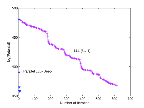
Figure 3: An example of the potential function against the number of iterations for standard LLL with $\delta=1$ and parallel LLL-deep.

As shown in Fig. 4(a), the proposed parallel LLL-deep has the advantage of a regular, modular structure, and further allows for pipeline implementation. Further, it is possible to run sorted GSO and size reduction simultaneously in Algorithm 6, as shown in Fig. 4(b). To do so, we just add Line 9 in sorted GSO (Algorithm 5), which will lead to the same reduced basis. It will cost approximately $n^{3}$ flops. Thus, the computational complexity of each super-iteration is roughly $3n^{3}$, $50\%$ higher than that of sorted GSO. Since sorted GSO and size reduction are computed simultaneously, the latency will be reduced. Further, both sorted GSO and size reduction themselves can be parallelized [47]. We can see that while the overall complexity might be $O(n^{4}\log n)$, the throughput and latency of Fig. 4(b) in a pipeline structure are similar to those of V-BLAST.

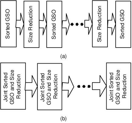
Figure 4: Fixed-complexity implementation of the LLL algorithm. (a) Separate sorted GSO and size reduction; (b) joint sorted GSO and size reduction.

V-B1 Using Sorted Cholesky Decomposition

The complexity of the proposed parallel LLL-deep in Fig. 4 mostly comes from repeated GSO. To reduce the complexity, we can replace it by sorted Cholesky decomposition [49]. This will yield the same reduced basis, but has lower computational complexity. The complexity of sorted Cholesky decomposition is approximately $n^{3}/3$ (the initial multiplication $\mathbf{A}=\mathbf{B}^{H}\mathbf{B}$ costs approximately $n^{3}$ due to symmetry), while that of sorted QR decomposition is approximately $2n^{3}$.

Since the sorted Cholesky decomposition was given for the dual basis in [49], for the sake of clarity we redescribe it in Algorithm 7. Here, $c_{m,n}$ is the $(m,n)$-th entry of $\mathbf{C}$, while $\overline{c_{m,n}}$ denotes its complex conjugate. For convenience, we also use MATLAB notation $c_{i:j,k}$ to denote a vector containing those elements of $\mathbf{C}$. When Algorithm 7 terminates, the lower triangular part of $\mathbf{C}$ is the Hermitian transpose of the R factor of the QR decomposition for the basis $\mathbf{B}$. Similarly, one can run sorted Cholesky decomposition and size reduction simultaneously.

Algorithm 7  Sorted Cholesky Decomposition

Input: Gram matrix $\mathbf{A}=\mathbf{B}^{H}\mathbf{B}$
Output: R factor for the sorted basis

1:  let $\mathbf{{C}}=\mathbf{A}$

2:  for $i=1,2,...,n$ do

3:     $k=\arg\min_{i\leq m\leq n}{a_{m,m}}$

4:     exchange the $i$ and $k$-th columns and rows of $\mathbf{{C}}$

5:     $c_{i,i}:=\sqrt{c_{i,i}}$

6:     $c_{i+1:n,i}:=\frac{c_{i+1:n,i}}{{c_{i,i}}}$

7:     for $j=i+1,...,n$ do

8:        $c_{j:n,j}:=c_{j:n,j}-c_{j:n,i}\overline{c_{j,i}}$

V-B2 Relation to V-BLAST and DOLLAR Detector

The V-BLAST ordering is a well known technique to improve performance of communication by pre-sorting the columns of a matrix [32]. It maximizes the length of the shortest Gram-Schmidt vector of $\mathbf{B}$ among all $n!$ possible orders. V-BLAST ordering starts from the last column of $\mathbf{B}$; it successively chooses the $i$-th Gram-Schmidt vector with the maximum length for $i=n,n-1,...,1$. Several $O(n^{3})$ algorithms have been proposed. One of them is obtained by applying sorted GSO to the dual lattice [49]. This results in significant computational savings because only a single GSO process is needed.

Now it is clear that the first iteration of parallel LLL-deep is very similar to the DOLLAR detector in [35], which is comprised of a sorted QR decomposition, a size reduction, and a V-BLAST sorting. Since V-BLAST sorting is very close to sorted QR decomposition, replacing V-BLAST ordering with sorted QR decomposition does not make much difference. In view of this, the DOLLAR detector can be seen as the first-order approximation of parallel LLL-deep, which explains its good performance. It can be seen from Fig. 3 that the first iteration appears to decrease the potential more than any other iterations. Of course, using just one iteration also limits the performance of the DOLLAR detector.

V-B3 Relation to Standard LLL and Some Variants

In fact, the inventors of the LLL algorithm already suggested to successively make $\|\mathbf{\hat{b}}_{1}\|,\|\mathbf{\hat{b}}_{2}\|,\cdots,\|\mathbf{\hat{b}}_{n}\|$ as small as possible [50], since they observed that shorter vectors among $\mathbf{\hat{b}}_{1},\mathbf{\hat{b}}_{2},\cdots,\mathbf{\hat{b}}_{n}$ typically appear at the end of the sequence. This idea is similar to sorted QR decomposition, but in the LLL algorithm it is implemented incrementally by means of swapping (i.e., in a bubble-sort fashion).

Joint sorting and reduction [51] is also similar to LLL-deep. It is well known that ordering can be used as a preprocessing step to speed up lattice reduction. A more natural approach is joint sorting and reduction [51] that uses modified GSO and when a new vector is picked it picks the one with the minimum norm (projected to the orthogonal complement of the basis vectors already reduced). That is, it runs sorted GSO only once.

Recently, Nguyen and Stehlé proposed a greedy algorithm for low-dimensional lattice reduction [52]. It computes a Minkowski-reduced basis up to dimension 4. Their algorithm is recursive; in each recursion, the basis vectors are ordered by increasing lengths. Obviously, following their idea, we can define another notion of lattice reduction where the basis vectors are sorted in increasing lengths and also size-reduced. The implementation of this algorithm resembles that of parallel LLL-deep. That is, such a basis can be obtained by alternatively sorting in lengths and size reduction. Using the same argument as that of LLL-deep, one can show that this algorithm will also terminate after a finite number of super-iterations. However, it seems difficult to prove any bounds for this algorithm.

V-B4 Reducing the Complexity of Sequential LLL-Deep

While the primary goal is to allow parallel pipeline hardware implementation, the proposed LLL-deep algorithm also has a computational advantage over the conventional LLL-deep algorithm even in a sequential computer for the first few iterations. We observed that running parallel LLL-deep crudely will not improve the speed. While parallel LLL-deep is quite effective at the early stage, keeping running it becomes wasteful at the late stage as the quality of the basis has improved a lot. In fact, updating occurs less frequently at the late stage; thus the standard serial version of LLL-deep will be faster. As a result, a hybrid strategy using parallel LLL-deep at the early stage and then switching to the serial version at the late stage will be more efficient. Parallel LLL-deep can be viewed as a preprocessing stage for such a hybrid strategy. One can run some numerical experiments to determine when is the best time to switch from parallel to sequential LLL-deep.

In Fig. 5, we show the average running time for LLL-deep for the complex MIMO lattice, on a notebook computer with Pentium Dual CPU working at 1.8 GHz. Sorted GSO is used. It is seen that the hybrid strategy can improve the speed by a factor up to 3 for $n\leq 50$.

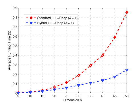
Figure 5: Average running time for standard and hybrid LLL-deep for the complex MIMO lattice. The number of iterations in parallel LLL-deep is set to 2.

V-C Bit Error Rate (BER) Performance

We evaluate the impact of a finite number of super-iterations on the performance of parallel LLL and LLL-deep. In the following simulations of the BER performance, we use MMSE-based lattice decoding and set $\delta=1$ in the complex LLL algorithm for the best performance.

Fig. 6 shows the performance of parallel effective LLL for different numbers of super-iterations for an $8\times 8$ MIMO system with 64-QAM modulation and SIC detection. The performance of ML detection is also shown as a benchmark of comparison. It is seen that increasing the number of iterations improves the BER performance; in particular, with 8 iterations, parallel effective LLL almost achieves the same performance as standard LLL. On the other hand, the returning SNR gain after the first few iterations is diminishing as the number of iterations increases.

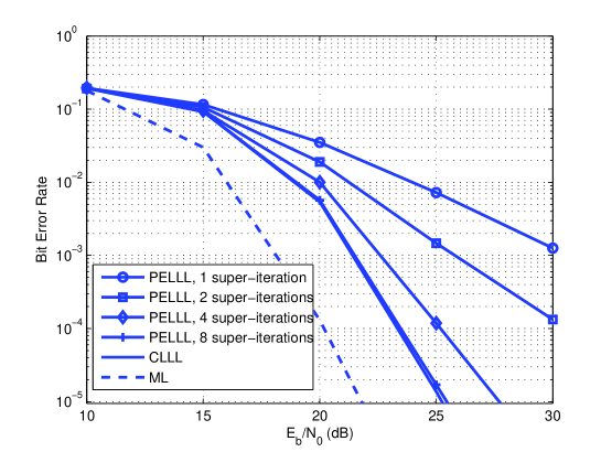
Figure 6: Performance of parallel effective LLL (PELLL) for a $8\times 8$ MIMO system with 64-QAM and SIC detection.

Fig. 7 shows the performance of parallel LLL-deep for an $8\times 8$ MIMO system with 64-QAM modulation and SIC detection. A similar trend is observed. Note that parallel LLL-deep with only one super-iteration, which essentially corresponds to the DOLLAR detector in [35], does not achieve full diversity, despite its good performance. Compared to Fig. 6, we can see that the performance is very similar in the end, but parallel LLL-deep seems to perform better in the first few super-iterations.

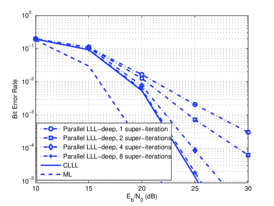
Figure 7: Performance of parallel LLL-deep for an $8\times 8$ MIMO system with 64-QAM and SIC detection.

VI Concluding Remarks

We have derived the $O(n^{4}\log n)$ average complexity of the LLL algorithm in MIMO communication. We also proposed the use of effective LLL that enjoys $O(n^{3}\log n)$ theoretic average complexity. Although in practice effective LLL does not significantly reduce the complexity, the $O(n^{3}\log n)$ theoretic bound improves our understanding of the complexity of LLL. To address the issue of variable complexity, we have proposed two parallel versions of the LLL algorithm that allow truncation after some super-iterations. Such truncation led to fixed-complexity approximation of the LLL algorithm. The first such algorithm was based on effective LLL, and we argued that it is sufficient to run $O(n\log n)$ super-iterations. The second was a parallel version of LLL-deep, which overcomes the limitation of the DOLLAR detector. We also showed that V-BLAST is a relative of LLL.

Finally, we point out some open questions.

A precise bound on the complexity of LLL remains to be found. The $O(n^{4}\log n)$ bound seems to be loose in MIMO communication.

Using effective LLL reduction may raise the concern of numerical stability, as the GS coefficients will grow. Although with the accuracy present in most floating-point implementations, this does not seem to cause a problem for the practical ranges of $n$ in MIMO communications, a rigorous study on this issue (e.g., following [40]) is a topic of future research.

Although for parallel effective LLL, we proved that the first basis vector is short after $O(n\log n)$ super-iterations, it remains to show in theory whether full diversity can be achieved or not. It is also an open question whether similar results exist for parallel LLL-deep.

Appendix A Relations Between Real and Complex LLL

A-A Reducedness

It is common in literature to convert the complex basis matrix ${\bf B}$ into a real matrix and then apply the standard real LLL algorithm. We shall analyze the relationship between this approach and complex LLL. There are many ways to convert ${\bf B}$ into a real matrix. One of them is to convert each element of ${\bf B}$ locally, i.e.,

$${\bf B_{\text{R}}}=\left[\begin{array}[]{ccc}\Re(b_{1,1})&-\Im(b_{1,1})&\cdots\\ \Im(b_{1,1})&\Re(b_{1,1})&\cdots\\ \cdots&\cdots&\ddots\\ \end{array}\right].$$ (28)

For convenience, we write this conversion as

$$\mathbf{B}_{\text{R}}=\mathcal{F}(\mathbf{B}).$$

Obviously, ${\bf B_{\text{R}}}$ is $2n$-dimensional if ${\bf B}$ is $n$-dimensional.

Another conversion is

$${\bf B}_{\text{R}}^{\prime}=\left[\begin{array}[]{cc}\Re({\bf B})&-\Im({\bf B})\\ \Im({\bf B})&\Re({\bf B})\\ \end{array}\right].$$ (29)

Correspondingly, we write this as

$$\mathbf{B}_{\text{R}}^{\prime}=\mathcal{F}^{\prime}(\mathbf{B}).$$

Note that when the real-valued LLL algorithm is applied to $\mathbf{B}_{\text{R}}$ or $\mathbf{B}_{\text{R}}^{\prime}$, the structures as above are generally not preserved.

Now suppose the complex matrix ${\bf B}$ has been complex LLL-reduced. We then expand the reduced ${\bf B}$ as in (28) or (29). What can be said about $\mathbf{B}_{\text{R}}$ and $\mathbf{B}_{\text{R}}^{\prime}$?

Lemma 2

Let $\mathbf{B}=\mathbf{\hat{B}}\mbox{\boldmath{$\mu$}}^{T}$ and $\mathbf{B}_{\text{R}}=\mathbf{\hat{B}}_{\text{R}}(\mbox{\boldmath{$\mu$}}_{\text{R}})^{T}$ be the Gram-Schmidt orthogonalization of the complex matrix $\mathbf{B}$ and its real counterpart $\mathbf{B}_{\text{R}}$, respectively. Then we have $\mathbf{\hat{B}}_{\text{R}}=\mathcal{F}(\mathbf{\hat{B}})$ and $\mbox{\boldmath{$\mu$}}_{\text{R}}=\mathcal{F}(\mbox{\boldmath{$\mu$}})$.

The proof is omitted. Lemma 2 says that the structure in (28) is preserved under Gram-Schmidt orthogonalization. Using this we now prove the following result.

Proposition 7

If $\mathbf{B}$ is reduced in the sense of complex LLL with parameter $\delta$ ($1/2<\delta\leq 1$), then $\mathbf{B}_{\text{R}}$ is reduced in the sense of real LLL with parameter $\delta-1/4$.

Proof:

First, note that $\|\mathbf{\hat{b}}_{\text{R},2i-1}\|=\|\mathbf{\hat{b}}_{\text{R},2i}\|=\|\mathbf{\hat{b}}_{i}\|$, and $\mbox{\boldmath{$\mu$}}_{\text{R}}$ looks like

$${\mbox{\boldmath{$\mu$}}}_{\text{R}}=\left[\begin{array}[]{ccccc}1&0&0&\cdots&\cdots\\ 0&1&0&\cdots&\cdots\\ \Re(\mu_{2,1})&-\Im(\mu_{2,1})&1&\cdots&\cdots\\ \Im(\mu_{2,1})&\Re(\mu_{2,1})&0&1&\cdots\\ \cdots&\cdots&\cdots&\cdots&\ddots\\ \end{array}\right].$$ (30)

Obviously the Lovász condition is satisfied by the $(2i-1)$ and $(2i)$-th column vectors of $\mathbf{B}_{\text{R}}$ because $\|\mathbf{\hat{b}}_{\text{R},2i}\|^{2}=\|\mathbf{\hat{b}}_{\text{R},2i-1}\|^{2}\geq(\delta-|\mu_{\text{R},2i,2i-1}|^{2})\|\mathbf{\hat{b}}_{\text{R},2i-1}\|^{2}$. Let us examine $(2i)$ and $(2i+1)$-th column vectors. From (3) we have

$$\begin{split}\|\mathbf{\hat{b}}_{\text{R},2i+1}\|^{2}&\geq(\delta-|\Re(\mu_{i+1,i})|^{2}-|\Im(\mu_{i+1,i})|^{2})\|\mathbf{\hat{b}}_{\text{R},2i}\|^{2}\\ &\geq(\delta-1/4-|\Im(\mu_{i+1,i})|^{2})\|\mathbf{\hat{b}}_{\text{R},2i}\|^{2}\\ &=(\delta-1/4-|\mu_{\text{R},2i+1,2i}|^{2})\|\mathbf{\hat{b}}_{\text{R},2i}\|^{2}.\end{split}$$ (31)

This proves the Proposition. ∎

Remark 8

It appears that little can be said about $\mathbf{B}_{\text{R}}^{\prime}$.

By Proposition 7, even if a 2-dimensional complex lattice $\mathbf{B}$ is Gauss-reduced (which is arguably the strongest reduction), its real equivalent $\mathbf{B}_{\text{R}}$ is not necessarily LLL-reduced with parameter $\delta=1$. It is easy to construct such a lattice

$$\left[\begin{array}[]{cc}1&0\\ 1/2+j/2&\sqrt{2}/2\\ \end{array}\right].$$

A-B Approximation factors

Let us compare the approximation factors for the first vectors $\mathbf{b}_{1}$ and $\mathbf{b}_{\text{R},1}$ in the reduced bases. Since $\det\mathbf{B}=\text{det}^{2}\mathbf{B}_{\text{R}}$ and the shortest nonzero vectors have the same length in the real and complex bases, we only need to compare $\alpha^{n-1}$ with $\beta^{2n-1}$. Recall that $\alpha=1/(\delta-1/2)$ and $\beta=1/(\delta-1/4)$. It is easy to check $\alpha\geq\beta^{2}$, because

$$(\delta-1/4)^{2}\geq\delta-1/2$$ (32)

where the equality holds if and only if $\delta=3/4$. Therefore, asymptotically, complex LLL has a larger approximation factor unless $\delta=3/4$. In fact, a minor difference between the error performances of real and complex LLL can be observed when $n$ becomes large (e.g., $n\geq 10$), although they are indistinguishable at small dimensions [26].

References

- [1] W. H. Mow, “Maximum likelihood sequence estimation from the lattice viewpoint,” IEEE Trans. Inform. Theory, vol. 40, pp. 1591–1600, Sept. 1994.
- [2] E. Viterbo and J. Boutros, “A universal lattice code decoder for fading channels,” IEEE Trans. Inform. Theory, vol. 45, pp. 1639–1642, July 1999.
- [3] M. O. Damen, H. E. Gamal, and G. Caire, “On maximum likelihood detection and the search for the closest lattice point,” IEEE Trans. Inform. Theory, vol. 49, pp. 2389–2402, Oct. 2003.
- [4] E. Agrell, T. Eriksson, A. Vardy, and K. Zeger, “Closest point search in lattices,” IEEE Trans. Inform. Theory, vol. 48, pp. 2201–2214, Aug. 2002.
- [5] U. Fincke and M. Pohst, “Improved methods for calculating vectors of short length in a lattice, including a complexity analysis,” Math. Comput., vol. 44, pp. 463–471, Apr. 1985.
- [6] J. Jaldén and B. Ottersen, “On the complexity of sphere decoding in digital communications,” IEEE Trans. Signal Processing, vol. 53, pp. 1474–1484, Apr. 2005.
- [7] F. Oggier, G. Rekaya, J.-C. Belfiore, and E. Viterbo, “Perfect space time block codes,” IEEE Trans. Inform. Theory, vol. 52, pp. 3885–3902, Sept. 2006.
- [8] B. M. Hochwald, C. B. Peel, and A. L. Swindlehurst, “A vector perturbation technique for near-capacity multiantenna multiuser communications-Part II: Perturbation,” IEEE Trans. Commun., vol. 53, pp. 537–544, Mar. 2005.
- [9] C. Ling, W. H. Mow, K. H. Li, and A. C. Kot, “Multiple-antenna differential lattice decoding,” IEEE J. Select. Areas Commun., vol. 23, pp. 1281–1289, Sept. 2005.
- [10] H. Yao and G. W. Wornell, “Lattice-reduction-aided detectors for MIMO communication systems,” in Proc. Globecom’02, Taipei, China, Nov. 2002, pp. 17–21.
- [11] C. Windpassinger and R. F. H. Fischer, “Low-complexity near-maximum-likelihood detection and precoding for MIMO systems using lattice reduction,” in Proc. IEEE Information Theory Workshop, Paris, France, Mar. 2003, pp. 345–348.
- [12] L. Babai, “On Lovász’ lattice reduction and the nearest lattice point problem,” Combinatorica, vol. 6, no. 1, pp. 1–13, 1986.
- [13] M. Taherzadeh, A. Mobasher, and A. K. Khandani, “LLL reduction achieves the receive diversity in MIMO decoding,” IEEE Trans. Inform. Theory, vol. 53, pp. 4801–4805, Dec. 2007.
- [14] X. Ma and W. Zhang, “Performance analysis for V-BLAST systems with lattice-reduction aided linear equalization,” IEEE Trans. Commun., vol. 56, pp. 309–318, Feb. 2008.
- [15] C. Ling, “On the proximity factors of lattice reduction-aided decoding,” IEEE Trans. Signal Processing, submitted for publication. [Online]. Available: http://www.commsp.ee.ic.ac.uk/ cling/
- [16] J. Jaldén and P. Elia, “LR-aided MMSE lattice decoding is DMT optimal for all approximately universal codes,” in Proc. Int. Symp. Inform. Theory (ISIT’09), Seoul, Korea, 2009.
- [17] D. Wuebben, R. Boehnke, V. Kuehn, and K. D. Kammeyer, “Near-maximum-likelihood detection of MIMO systems using MMSE-based lattice reduction,” in Proc. IEEE Int. Conf. Commun. (ICC’04), Paris, France, June 2004, pp. 798–802.
- [18] S. Liu, C. Ling, and D. Stehlé, “Randomized lattice decoding,” IEEE Trans. Inform. Theory, submitted for publication. [Online]. Available: http://arxiv.org/abs/1003.0064
- [19] L. Luzzi, G. R.-B. Othman, and J.-C. Belfiore, “Augmented lattice reduction for MIMO decoding,” IEEE Trans. Wireless Commun., submitted for publication. [Online]. Available: http://arxiv.org/abs/1001.1625
- [20] A. K. Lenstra, J. H. W. Lenstra, and L. Lovász, “Factoring polynomials with rational coefficients,” Math. Ann., vol. 261, pp. 515–534, 1982.
- [21] C. P. Schnorr and M. Euchner, “Lattice basis reduction: Improved practical algorithms and solving subset sum problems,” Math. Program., vol. 66, pp. 181–191, 1994.
- [22] N. Gama and P. Q. Nguyen, “Predicting lattice reduction,” in Proc. Eurocrypt ’08. Springer, 2008.
- [23] H. Napias, “A generalization of the LLL-algorithm over Euclidean rings or orders,” Journal de The’orie des Nombres de Bordeaux, pp. 387–396, 1996.
- [24] N. Howgrave-Graham, “Computational mathematics inspired by RSA,” PhD dissertation, University of Bath, Department of Computer Science, Bath, UK, 1998.
- [25] W. H. Mow, “Universal lattice decoding: Principle and recent advances,” Wireless Communications and Mobile Computing, vol. 3, pp. 553–569, Aug. 2003.
- [26] Y. H. Gan, C. Ling, and W. H. Mow, “Complex lattice reduction algorithm for low-complexity full-diversity MIMO detection,” IEEE Trans. Signal Processing, vol. 57, pp. 2701–2710, July 2009.
- [27] H. Daude and B. Vallee, “An upper bound on the average number of iterations of the LLL algoirthm,” Theor. Comput. Sci., vol. 123, pp. 95–115, 1994.
- [28] C. Ling and N. Howgrave-Graham, “Effective LLL reduction for lattice decoding,” in Proc. Int. Symp. Inform. Theory (ISIT’07), Nice, France, June 2007.
- [29] N. Howgrave-Graham, “Finding small roots of univariate modular equations revisited,” in Proc. the 6th IMA Int. Conf. Crypt. Coding, 1997, pp. 131–142.
- [30] W. H. Mow, “Maximum likelihood sequence estimation from the lattice viewpoint,” MPhil dissertation, Chinese University of Hong Kong, Department of Information Engineering, Hong Kong, China, June 1991. [Online]. Available: http://www.ece.ust.hk/ eewhmow/
- [31] J. Jaldén, D. Seethaler, and G. Matz, “Worst- and average-case complexity of LLL lattice reduction in MIMO wireless systems,” in Proc. ICASSP’08, Las Vegas, NV, US, 2008, pp. 2685–2688.
- [32] P. W. Wolniansky, G. J. Foschini, G. D. Golden, and R. A. Valenzuela, “V-BLAST: An architecture for realizing very high data rates over richscattering wireless channel,” in Proc. Int. Symp. Signals, Syst., Electron. (ISSSE’98), Pisa, Italy, Sept. 1998, pp. 295–300.
- [33] H. Vetter, V. Ponnampalam, M. Sandell, and P. A. Hoeher, “Fixed complexity LLL algorithm,” IEEE Trans. Signal Processing, vol. 57, pp. 1634–1637, Apr. 2009.
- [34] C. Ling and W. H. Mow, “A unified view of sorting in lattice reduction: From V-BLAST to LLL and beyond,” in Proc. IEEE Inform. Theory Workshop 2009 (ITW’09), Taormina, Italy, Oct. 2009.
- [35] D. W. Waters and J. R. Barry, “A reduced-complexity lattice-aided decision-feedback detector,” in Proc. IEEE International Conference on Wireless Networks, Communications, and Mobile Computing (WirelessComm’2005), Maui, Hawaii, June 2005.
- [36] J. H. Conway and N. J. A. Sloane, Sphere Packings, Lattices, and Groups, 2nd ed. New York: Springer-Verlag, 1993.
- [37] G. H. Golub and C. F. V. Loan, Matrix Computations, 3rd ed. Baltimore, MD: Johns Hopkins University Press, 1996.
- [38] A. Akhavi, “The optimal LLL algorithm is still polynomial in fixed dimension,” Theoretical Computer Science, vol. 297, pp. 3–23, Mar. 2003.
- [39] H. W. Lenstra, “Flags and lattice basis reduction,” in Proc. 3rd Europ. Congr. Math., Basel, 2000.
- [40] P. Nguyen and D. Stehlé, “Floating-point LLL revisited,” Eurocrypt’05, Aarhus, Denmark, May 22-26, 2005.
- [41] N. R. Goodman, “Statistical analysis based on a certain multivariate complex gaussian distribution (an introduction),” Ann. Math. Statist., vol. 34, pp. 152–177, Mar. 1963.
- [42] J. C. Lagarias, W. H. Lenstra, and C. P. Schnorr, “Korkin-Zolotarev bases and successive minima of a lattice and its reciprocal lattice,” Combinatorica, vol. 10, no. 4, pp. 333–348, 1990.
- [43] C. Windpassinger, R. Fischer, and J. B. Huber, “Lattice-reduction-aided broadcast precoding,” IEEE Trans. Commun., vol. 52, pp. 2057–2060, Dec. 2004.
- [44] A. Storjohann, “Faster algorithms for integer basis reduction,” ETH-Zurich, Department of Computer Science, Zurich, Switzerland, Tech. Rep. 249, 1996.
- [45] G. Villard, “Parallel lattice basis reduction,” in Proc. ACM ISSAC’92, CA, 1992, pp. 269–277.
- [46] N.-C. Wang, E. Biglieri, and K. Yao, “A systolic array for linear MIMO detection based on an all-swap lattice reduction algorithm,” in Proc. ICASSP’09, Taipei, China, 2009, pp. 2461–2464.
- [47] G. Heckler and L. Thiele, “Complexity analysis of a parallel lattice basis reduction algorithm,” SIAM J. Comput., vol. 27, pp. 1295–1302, Oct. 1998.
- [48] D. Wubben, R. Bohnke, J. Rinas, V. Kuhn, and K. Kammeyer, “Efficient algorithm for decoding layered space-time codes,” Electron. Lett., vol. 37, pp. 1348–1350, Oct. 2001.
- [49] C. Ling, W. H. Mow, and L. Gan, “Dual-lattice algorithms and partial lattice reduction for SIC-based MIMO detection,” IEEE J. Select. Topics Signal Processing, vol. 3, pp. 975–985, Dec. 2009.
- [50] L. Lovász, An Algorithmic Theory of Numbers, Graphs and Convexity. Pennsylvania: Society for Industrial and Applied Mathematics, 1986.
- [51] Y. H. Gan and W. H. Mow, “Novel joint sorting and reduction technique for delay-constrained LLL-aided MIMO detection,” IEEE Signal Processing Lett., vol. 15, pp. 194–197, 2008.
- [52] P. Nguyen and D. Stehlé, “Low-dimensional lattice basis reduction revisited,” in Proceedings of the 6th Algorithmic Number Theory Symposium (ANTS VI), ser. Lecture Notes in Computer Science, vol. 3076. Springer-Verlag, 2004, pp. 338–357.