Spatially and Spectrally Resolved Hydrogen Gas within 0.1 AU of T Tauri and Herbig Ae/Be Stars

Abstract

We present near-infrared observations of T Tauri and Herbig Ae/Be stars with a spatial resolution of a few milli-arcseconds and a spectral resolution of $\sim 2000$. Our observations spatially resolve gas and dust in the inner regions of protoplanetary disks, and spectrally resolve broad-linewidth emission from the Br$\gamma$ transition of hydrogen gas. We use the technique of spectro-astrometry to determine centroids of different velocity components of this gaseous emission at a precision orders of magnitude better than the angular resolution. In all sources, we find the gaseous emission to be more compact than or distributed on similar spatial scales to the dust emission. We attempt to fit the data with models including both dust and Br$\gamma$–emitting gas, and we consider both disk and infall/outflow morphologies for the gaseous matter. In most cases where we can distinguish between these two models, the data show a preference for infall/outflow models. In all cases, our data appear consistent with the presence of some gas at stellocentric radii of $\sim 0.01$ AU. Our findings support the hypothesis that Br$\gamma$ emission generally traces magnetospherically driven accretion and/or outflows in young star/disk systems.

1 Introduction

Protoplanetary disks play an integral part in the formation of both stars and planets. Disks provide a reservoir from which stars and planets accrete material, and a knowledge of the structure of inner regions of disks is needed to understand the star/disk interface as well as planet formation in disk ‘terrestrial’ regions.

Near-infrared interferometry enables spatially resolved observations of sub-AU-sized regions of protoplanetary disks in nearby star-forming regions (see Millan-Gabet et al. 2007, or Dullemond & Monnier 2010 for recent reviews). These observations have enabled direct constraints on the distribution and temperature of dust in terrestrial planet forming regions, and have more recently begun to probe gaseous emission as well (Eisner et al. 2007a; Eisner 2007; Malbet et al. 2007; Tatulli et al. 2007; Tannirkulam et al. 2008; Tatulli et al. 2008; Isella et al. 2008; Kraus et al. 2008; Eisner et al. 2009). Spatially resolved observations remove ambiguities inherent in previous modeling of spatially unresolved spectral energy distributions (e.g., Bertout et al. 1988; Hillenbrand et al. 1992) or gaseous emission lines (e.g., Edwards et al. 1994; Najita et al. 1996), and allow critical tests of these models.

Spectrally and spatially resolved observations of hydrogen gas have the potential to constrain how inner disk material accretes onto the central star or leaves the system (carrying away angular momentum) in outflows. Because hydrogen in accretion flows or in the innermost regions of outflows can be ionized, it may emit via a number of electronic transitions as recently recombined atoms cascade down to the ground state. The Br$\gamma$ transition, from the $n=7\rightarrow 4$ electronic states, produces a spectral line at 2.1662 $\mu$m, and can be observed with infrared interferometers. This line has been shown to be strongly correlated with accretion onto young stars (Muzerolle et al. 1998). While Balmer series hydrogen lines often show P Cygni profiles associated with winds (or a combination of winds and infall; e.g., Kurosawa et al. 2006), Br$\gamma$ line profiles are often more consistent with infall kinematics (e.g., Najita et al. 1996).

Accretion is thought to occur by magnetospheric accretion in low-mass stars (e.g., Königl 1991). Viscous accretion of gas brings material through the disk to the magnetospheric radius where stellar magnetic fields exert outward pressure to balance the inward pressure of accretion; gas is then funneled along magnetic field lines onto high-latitude regions of the star. The interaction of the stellar magnetic field and the disk may also lead to the launching of outflows near this magnetospheric radius (e.g., Shu et al. 1994) or from stellocentric radii of an AU or more (e.g., Konigl & Pudritz 2000). An alternative to the magnetospheric accretion picture (that may operate in higher-mass stars; e.g., Eisner et al. 2004) is disk/boundary layer accretion. Matter is accreted viscously through a disk all the way to the star, at which point a shock forms due to the large difference in velocities between the Keplerian disk and rotating stellar surface (e.g., Lynden-Bell & Pringle 1974).

Previous, spatially resolved observations of protoplanetary disks generally found Br$\gamma$ emission to be more compactly distributed than continuum emission (Eisner 2007; Kraus et al. 2008; Eisner et al. 2009), although more extended distributions were seen in a few cases (Malbet et al. 2007; Tatulli et al. 2007). For the subset of observations where the Br$\gamma$ line was spectrally resolved, Kraus et al. (2008) claimed that only one object appears compatible with a model where the Br$\gamma$ emission arises in an infalling accretion flow. For the other four objects in their sample, Kraus et al. (2008) suggested that this emission may trace extended disk winds (as described in, e.g., Konigl & Pudritz 2000). However, this sample was limited to a few bright A and B stars, which may not be representative of most young stars.

Here we use the Keck Interferometer (KI) to spatially and spectrally resolve gas within 1 AU of a sample of fifteen young stars spanning a mass range from $\sim 0.5$–10 M_⊙. These observations expand the previous sample by a factor of 3 in number and by an order of magnitude in mass range. We determine the spatial distribution and velocity structure of the Br$\gamma$-emitting gas for this sample. We investigate how these properties depend on stellar mass or accretion rate, and compare our findings to models of accretion and outflow.

2 Observations and Data Reduction

2.1 Sample

We selected a sample of young stars (Table Spatially and Spectrally Resolved Hydrogen Gas within 0.1 AU of T Tauri and Herbig Ae/Be Stars) known to be surrounded by protoplanetary disks, all of which have been observed previously at near-IR wavelengths with long-baseline interferometers (Millan-Gabet et al. 2001; Eisner et al. 2004, 2005, 2007c; Colavita et al. 2003; Monnier et al. 2005; Akeson et al. 2005a, b). All targets have been previously spatially resolved in the near-IR.

Our sample (Table Spatially and Spectrally Resolved Hydrogen Gas within 0.1 AU of T Tauri and Herbig Ae/Be Stars) includes seven T Tauri stars, pre-main-sequence analogs of solar-type stars like our own sun; five Herbig Ae/Be stars, 2–10 M_⊙ pre-main-sequence stars; and three stars (AS 353, V1057 Cyg, and V1331 Cyg) with heavily veiled stellar photospheres whose spectral types are uncertain. Our experimental setup imposes limiting magnitudes of $K\sim 7$ at near-IR wavelengths and $V\sim 12$ at optical wavelengths. We also require that sources be at zenith angles of less than $\sim 50^{\circ}$, which excludes from our sample any sources with $\delta\lesssim-35^{\circ}$.

The sample was selected to satisfy these criteria, and includes most T Tauri stars that could be observed, focusing on those that are known to emit Br$\gamma$ and/or CO overtone emission (e.g., Folha & Emerson 2001; Carr 1989; Najita et al. 1996, 2007). Two sources in our sample are actually fainter than the limiting system magnitudes at $K$-band: AS 353 and V1331 Cyg. We included these because of their strong, previously observed CO overtone emission (e.g., Carr 1989). However, as we discuss below, we were unable to obtain high quality measurements for these fainter objects. Finally, we included several brighter Herbig Ae/Be stars that expanded the stellar mass range of the sample.

2.2 Experimental Setup

KI is a fringe-tracking long baseline near-IR Michelson interferometer combining light from the two 10-m Keck apertures (Colavita & Wizinowich 2003; Colavita et al. 2003). Each of the 10-m apertures is equipped with a natural guide star adaptive optics (NGS-AO) system that corrects phase errors caused by atmospheric turbulence across each telescope pupil, and thereby maintains spatial coherence of the light from the source across each aperture. The NGS-AO systems require sources with $R$ magnitudes brighter than $\sim 12$. Optical beam-trains transport the light from each Keck aperture down into a tunnel connecting the two Kecks and to a set of beam combination optics.

We used the “self phase referencing”(SPR) mode of KI, implemented as part of the ASTrometric and phase-Referenced Astronomy (ASTRA) program (see Woillez et al. 2010). The SPR mode introduces a split in the beams from each aperture, immediately before the fast delay line optics. 55% of the light is passed down the “primary” channel, which consists of the normal KI optics used in the standard $V^{2}$ mode. Of the remaining 45%, 20% of the light is split off to the “secondary” fast delay lines (which are generally used as part of the KI Nuller), and ultimately sent to a second beam-combining table and detector. Each of the detectors consists of a HAWAII array.

For both primary and secondary sides, interferometric fringes are measured by modulating the relative delay of the two input beams and then measuring the modulated intensity level of the combined beams during four “ABCD” detector reads (Colavita 1999). Each read has an integration time of 2 ms. The measured intensities in these reads are used to determine atmosphere-induced fringe motions, and a servo loop removes these motions to keep the fringes centered near zero phase.

For the secondary side, a servo loop uses the phase information measured on the primary side to stabilize the atmospheric phase motions, and we can thus use longer modulation periods (and hence integration times). We use integration times between 0.5 and 2 s, approximately 1,000 times longer than possible with the uncorrected primary side. While integrations longer than 2 s are possible, observations at wavelengths longer than 2 $\mu$m become background-limited in this regime.

In front of the secondary detector is a grism. This grism consists of a prism made of S-FTM16 glass, with refractive index$=$1.56 and an apex angle of 36.8^∘; and an epoxy grating with 150 grooves per mm and a blaze angle of 36.8^∘. Used in first-order, the grism passes the entire $K$-band with a dispersion of $\lambda/\Delta\lambda\approx 2000$. This spectral resolution is confirmed with measurements of a neon lamp spectrum. Note, however, that the lines are not fully Nyquist sampled with our detector; spectra are Nyquist sampled at a resolution of $\sim 1000$. Neon lamp spectra and/or Fourier Transform Spectroscopy are also used to determine the wavelength scale for each night of observed data. While the entire $K$-band falls on the detector, vignetting in the camera leads to lower throughput toward the band edges. The effective bandpass of our observations is approximately 2.05 to 2.35 $\mu$m.

In this paper we focus on Br$\gamma$ emission, which fills only a small portion of the $K$-band. Our measurements actually cover other interesting spectral regions that include significant opacity from H₂O and CO transitions. We defer discussion of these spectral regions to a later paper.

2.3 Observations

We obtained Keck Interferometer (KI) observations of our sample on UT 2008 April 25, 2008 November 17, 2008 November 18, and 2009 July 15 (see Table 2). The first of these nights was actually the commissioning night of the SPR mode, and so we observed a number of unresolved calibrator stars and known, strong Br$\gamma$ emitters, to use for system characterization. The analysis of these initial data is presented in separate papers (Woillez et al. 2010; Pott et al. 2010). When observing our sample, targets were interleaved with calibrators every 10–15 minutes.

2.4 $V^{2}$ Calibration

We measured squared visibilities ($V^{2}$) for our targets and calibrator stars in each of the 330 spectral channels across the $K$-band provided by the grism. The calibrator stars are main sequence stars, with known parallaxes, whose $K$ magnitudes are within 0.5 mags of the target $K$ magnitudes (Table Spatially and Spectrally Resolved Hydrogen Gas within 0.1 AU of T Tauri and Herbig Ae/Be Stars). The system visibility (i.e., the point source response of the interferometer) was measured using observations of these calibrators, whose angular sizes were estimated by fitting blackbodies to literature photometry. These size estimates are not crucial since the calibrators are unresolved (i.e., their angular sizes are much smaller than the interferometric fringe spacing) in almost all cases. HD 163955, a calibrator for MWC 275, is mildly resolved; we account for this when computing the system visibility.

We calculated the system visibility appropriate to each target scan by weighting the calibrator data by the internal scatter and the temporal and angular proximity to the target data (Boden et al. 1998). For comparison, we also computed the straight average of the $V^{2}$ for all calibrators used for a given source, and the system visibility for the calibrator observations closest in time. These methods all produce results consistent within the measurement uncertainties. We adopt the first method in the analysis that follows.

Source and calibrator data were corrected for standard detection biases as described by Colavita (1999) and averaged into 5 s blocks. Calibrated $V^{2}$ were then computed by dividing the average measured $V^{2}$ over 130 s scans (consisting of 5 s sub-blocks) for targets by the average system visibility. Uncertainties are given by the quadrature addition of the internal scatter in the target data and the uncertainty in the system visibility. We average together all of the calibrated data for a given source to produce a single measurement of $V^{2}$ in each spectral channel. The observations of our targets typically spanned $\lesssim 1$ hour, and the averaging therefore has a small effect on the uv coverage.

As seen in previous observations with a lower-dispersion grism at KI (Eisner et al. 2007b), we find channel-to-channel uncertainties of a few percent or less in our data. Here we estimate these uncertainties by computing the standard deviation of $V^{2}$ measured in a spectral region spanning 2.2 to 2.25 $\mu$m. This region typically has good signal-to-noise, and does not contain signal from Br$\gamma$ emission or absorption.

The normalization of $V^{2}$ versus wavelength (i.e., the average value of $V^{2}$ across the band) has an additional uncertainty of $\sim 3\%$. We ignore this in our analysis since it does not affect the relative measurements of various channels.

2.5 Differential Phase Calibration

The “ABCD” reads are used to calculate the phase of interference fringes recorded in both the primary channel (as described in §2.2) and in the secondary channel. Infrared interferometers generally do not measure phase information that is intrinsic to the target, because rapid atmospheric phase distortions scramble the phase of the “pristine” wavefronts emitted by the source (e.g., Monnier 2007). However, with our SPR observations the atmospheric phase distortions are measured by the primary fringe tracker, and these phase motions are subtracted from the secondary side. Furthermore, for the dispersed fringes on the secondary side, any residual atmospheric phase motions would affect the fringes in each channel (approximately) the same way, and so the differential phase ($\Delta\phi$) across the observed spectrum is intrinsic to the source.

Raw phases are measured in the same “ABCD” reads used to determine $V^{2}$. These phases are then de-rotated so that the average phase of all channels is zero. Next, the phases versus wavelength are unwrapped to eliminate any 180^∘ jumps. After computing weighted average differential phases for each target and calibrator scan, we determine a “system differential phase” using similar weighting employed above to calculate the system visibility.

The system differential phase is subtracted from the target differential phase. Since targets and calibrators are observed at similar airmasses, this calibration procedure removes most atmospheric and instrumental refraction effects. Finally, we remove any residual slope in the differential phase spectrum, since we can not distinguish instrumental slopes from those intrinsic to the target signal. Since we are focused on a small spectral region around the Br$\gamma$ feature, we are largely insensitive to errors in these calibrations.

We estimate the uncertainty on the differential phase measurements by taking the standard deviation of measurements in a spectral region between 2.2 and 2.25 $\mu$m (as we did for $V^{2}$ above). The errors derived from the data are typically $\lesssim 1^{\circ}$, although the faintest objects in our sample exhibit somewhat larger uncertainties.

2.6 Flux Calibration

We used the count rates in each channel observed during “foreground integrations” (Colavita 1999) to recover crude spectra for our targets. These spectra are measured when no fringes are present, and include all flux measured within the $\sim 50$ mas diameter of the instrumental field of view. We divided the measured flux versus wavelength for our targets by the observed fluxes from the calibrator stars, using calibrator scans nearest in time to given target scans, and then multiplied the results by template spectra suitable for the spectral types of the calibrators.

We used Nextgen stellar atmosphere models (Hauschildt et al. 1999) as templates. These model spectra are computed at a resolution of 2 Å(more than five times finer than the resolution of our data) for stars with effective temperatures up to 10,000 K. They are thus suitable templates to be used with our calibrator stars (see Table Spatially and Spectrally Resolved Hydrogen Gas within 0.1 AU of T Tauri and Herbig Ae/Be Stars).

Tests of our calibration procedure for main sequence stars of known spectral type, calibrated using other calibrator stars, indicate channel-to-channel uncertainties of a few percent. Similar uncertainties are found by calculating the standard deviation in a spectral region adjacent to Br$\gamma$; we adopt these uncertainties for the analysis presented below. While we also see evidence for uncertainties in the spectral slope across the $K$-band (the slope varies from one observation to the next), we ignore these here since they do not affect the narrow-band data in the Br$\gamma$ spectral region.

2.7 Separating Stellar and Circumstellar Components

The fluxes, squared visibilities, and differential phases described above contain contributions from both circumstellar material and central stars. Since our interest here is in the circumstellar matter, we remove the stellar component of the measurements before proceeding.

Decomposition of the spectrum into stellar and circumstellar components is straightforward as long as the ratio of circumstellar-to-stellar flux is known at each observed wavelength. We estimate the circumstellar-to-stellar flux ratio at each observed wavelength following Eisner et al. (2009). We use stellar radii, effective temperatures, distances, and extinctions (assuming the reddening law of Steenman & Thé (1991)) from the literature (Hessman & Guenther 1997; Monin et al. 1998; White & Ghez 2001; Muzerolle et al. 2003; Eisner et al. 2004, 2005; Monnier et al. 2005, 2006; Bertout et al. 2007) to fit the stellar photosphere. The Nextgen models described in §2.6 are then used to determine the stellar fluxes at each of our observed wavelengths. These models are suitable for all of our stars except MWC 1080, whose effective temperature is substantially higher than the 10,000 K maximum of the Nextgen models. Such hot stars typically have shallower Br$\gamma$ absorption than cooler A stars, since the H ionization fraction in the stellar photosphere is higher. Thus, the circumstellar Br$\gamma$ spectrum may underestimate the true line-to-continuum ratio.

For AS 353A, V1331 Cyg, and V1057 Cyg, whose stellar photospheres are effectively invisible, we can not reliably estimate the circumstellar-to-stellar flux ratios. For these objects we assume that 100% of the $K$-band flux arises from the circumstellar environments. This assumption is consistent with previous spectroscopic observations of these objects (Eisloeffel et al. 1990; Herbig & Jones 1983; Eisner et al. 2007c; Hartmann et al. 2004).

To estimate the circumstellar components of the $V^{2}$ and $\Delta\phi$, we consider the contribution of the star to the complex visibilities:

$$V_{\rm meas}e^{i\Delta\phi_{\rm meas}}=\frac{F_{\ast}V_{\ast}e^{i\Delta\phi_{\ast}}+F_{\rm disk}V_{\rm disk}e^{i\Delta\phi_{\rm disk}}}{F_{\ast}+F_{\rm disk}}.$$ (1)

Here, $V_{\rm meas}=\sqrt{V^{2}_{\rm meas}}$, $F_{\ast}$ and $F_{\rm disk}$ are the stellar and circumstellar fluxes (determined above), and $V_{\ast}$ and $V_{\rm disk}$ are the stellar and circumstellar components contributing to the measured visibilities. Assuming the central star is unresolved and at the photo-center of the continuum emission, this can be simplified to

$$V_{\rm meas}e^{i\Delta\phi_{\rm meas}}=\frac{F_{\ast}+F_{\rm disk}V_{\rm disk}e^{i\Delta\phi_{\rm disk}}}{F_{\ast}+F_{\rm disk}}.$$ (2)

The real and imaginary parts of Equation 2 provide two equations, which can be solved for the two unknown quantities $V_{\rm disk}$ and $\Delta\phi_{\rm disk}$:

$$\Delta\phi_{\rm disk}=\tan^{-1}\left[\frac{V_{\rm meas}\sin(\Delta\phi_{\rm meas})(F_{\ast}+F_{\rm disk})}{V_{\rm meas}\cos(\Delta\phi_{\rm meas})(F_{\ast}+F_{\rm disk})-F_{\ast}}\right],$$ (3)

$$V_{\rm disk}=V_{\rm meas}\frac{\sin(\Delta\phi_{\rm meas})}{\sin(\Delta\phi_{\rm disk})}\left(\frac{F_{\ast}+F_{\rm disk}}{F_{\rm disk}}\right).$$ (4)

We use Equations 3 and 4 to compute the squared visibilities and differential phases corresponding to the circumstellar matter. However, we note that if the differential phases are small ($\ll 1$ rad), we can simplify these equations to somewhat more intuitive forms using the small angle approximation:

$$V_{\rm disk}=\frac{V_{\rm meas}(1+F_{\rm disk}/F_{\ast})-1}{F_{\rm disk}/F_{\ast}},$$ (5)

$$\Delta\phi_{\rm disk}=\frac{\Delta\phi_{\rm meas}\left(1+V_{\rm disk}F_{\rm disk}/F_{\ast}\right)}{V_{\rm disk}F_{\rm disk}/F_{\ast}}.$$ (6)

This assumption is equivalent to assuming that the differential phase is linearly related to the centroid offset, which is true for unresolved or marginally resolved structures:

$$\Delta\theta=\Delta\phi\frac{\lambda}{2\pi B},$$ (7)

where $\lambda$ is the observed wavelength and $B$ is the projected baseline length.

The uncertainties on $V^{2}_{\rm disk}$ and $\Delta\phi_{\rm disk}$ are computed from the uncertainties in $V^{2}_{\rm meas}$ or $\Delta\phi_{\rm meas}$ and an assumed uncertainty of 20% on the circumstellar-to-stellar flux ratio. We fit our models for the circumstellar emission to $F_{\rm disk}$, $V^{2}_{\rm disk}$, and $\Delta\phi_{\rm disk}$ below.

2.8 General Features of Calibrated Data

Figure 1 shows the fluxes in the Br$\gamma$ spectral region, calibrated with the procedure outlined in §2.6. Since many of our targets are early-type stars, which exhibit photospheric Br$\gamma$ absorption, we also plot in Figure 1 spectra from which the stellar contribution has been removed (§2.7). All of our targets except one show evidence of circumstellar Br$\gamma$ emission; in V1057 Cyg, Br$\gamma$ appears in absorption. In the analysis presented below we will focus on the remaining fourteen objects that exhibit Br$\gamma$ emission.

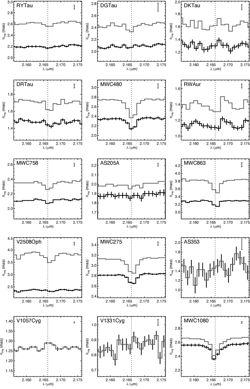
Figure 2: Uniform ring angular diameters of our sample, plotted in the spectral region around Br$\gamma$. Angular sizes computed directly from the observed $V^{2}$ are plotted with black histograms. Angular sizes of only the circumstellar emission, determined using the procedure described in §2.7, are shown with gray histograms.

To better illustrate the behavior of $V^{2}$ versus wavelength, we fit the $V^{2}$ data for each source, in each channel, with a simple uniform ring model (e.g., Eisner et al. 2004). The results, shown in Figure 2, give the “spectral size distribution” of the emission, illustrating how the spatial scale of the near-IR emission depends on wavelength. Figure 2 also shows the estimated angular size of only the circumstellar emission, calculated as described in §2.7

Figure 2 shows that the angular diameter of the near-IR emission changes across the spectral region of Br$\gamma$ emission in most of our target objects. While more compact sizes of Br$\gamma$ emission relative to continuum emission have been previously reported for a number of these objects (Eisner 2007; Eisner et al. 2009), here we resolve the size versus wavelength spectrally across the Br$\gamma$ feature. This augments the small number of existing measurements of this kind, since our sample only has an overlap of one with previous observations at similar spectral resolution (Kraus et al. 2008).

In all of our targets, the Br$\gamma$ emission appears either more compactly distributed than the surrounding continuum emission, or distributed on similar spatial scales. Using Equations 3 and 4, but with the line-to-continuum flux ratio in each spectral channel in lieu of the circumstellar-to-stellar flux ratios, we can compute the $V^{2}$ for the Br$\gamma$-emitting gas. Fitting this $V^{2}$ with a uniform ring model, we can derive simple size estimates. In particular, we fit a uniform ring model to the peak channel; since this is the lowest velocity material, it should also be the most extended and should thus trace approximately the full extent of the Br$\gamma$–emitting gas.

In Table 3, we compare the derived uniform ring sizes for the Br$\gamma$ emitting region with those of the continuum. Table 3 confirms the suggestion, based on Figure 2, that the Br$\gamma$ emission is more compact than, or distributed on similar scales to, the continuum emission for all objects in our sample. Furthermore, we see that in a number of cases, the inferred size of the Br$\gamma$ emission is $\lesssim 0.1$ mas, corresponding to radii $\lesssim 0.01$ AU for our targets.

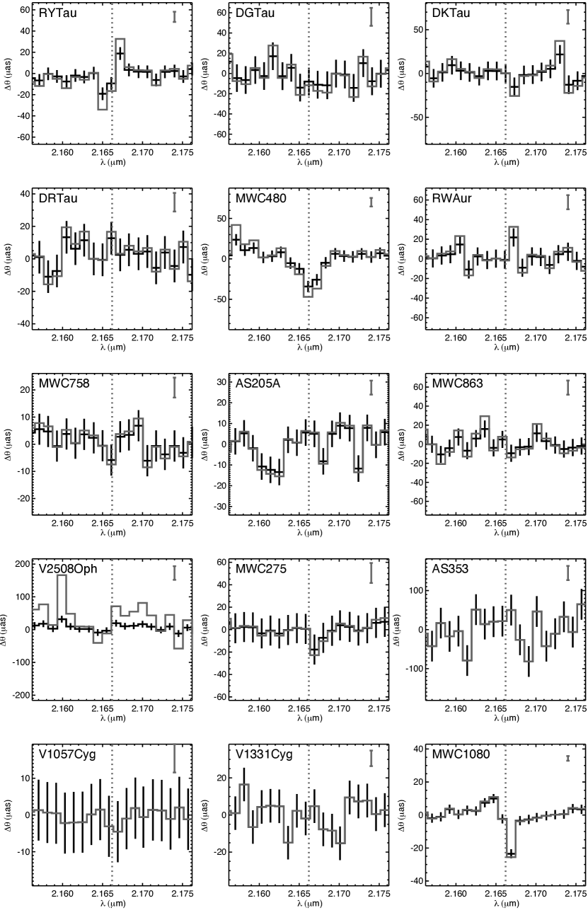
Figure 3: Centroid offsets of our sample, plotted in the spectral region around Br$\gamma$. Black histograms show the offsets derived for the observed data, and gray histograms show the centroid offsets for the circumstellar component of the emission.

To facilitate interpretation of the differential phase data, we convert the $\Delta\phi$ values into centroid offsets (Equation 7). Since KI consists of a single baseline, and we observe our targets with a limited $uv$ range, the derived centroid offsets are essentially projections onto a single position angle on the sky for a given object. The centroid offsets versus wavelength for our sample are plotted in Figure 3.

In most cases, no clear signals are seen in the differential phase data above the uncertainty level. However, a few objects display deviations from the mean phase at the wavelength of the Br$\gamma$ transition. Objects with clear signals are generally the brightest objects in our sample (RY Tau, MWC 480, MWC 275, and MWC 1080). The differential phase data is noisier and less reliable for fainter sources. For example, while AS 205 exhibits features in the differential phases (not at the Br$\gamma$ wavelength) that appear significant, these may be spurious signals for this fainter object.

3 Modeling

In this section we use our flux, $V^{2}$, and differential phase measurements, after removal of the stellar components (§2.7) to constrain the distribution of dust and gas around our sample stars. In §3.1, we consider a Keplerian disk model with a rotating, gaseous disk extending from some inner radius out to the dust sublimation radius, where a ring of continuum emission resides. In §3.2, we replace the rotating, gaseous disk with a compact, bipolar infall/outflow structure.

In these models we make the simple assumption that continuum emission is confined to a ring whose annular width is 20% of its inner radius. This assumption makes sense if the continuum emission traces dust, since most of the emission will come from radii near the sublimation point of silicate dust (Dullemond et al. 2001; Isella & Natta 2005). However, previous work has shown that inner disk gas or highly refractory dust, on smaller scales than the bulk of the dust emission, also produces continuum emission (e.g., Tannirkulam et al. 2008; Eisner et al. 2009; Benisty et al. 2010). This compact continuum emission can lead to underestimated sizes for the (bulk) dust distribution. However, since we are focused on the line emission, we are not concerned with such potential errors. The assumption that continuum emission lies in a single ring should not affect inferred constraints on the Br$\gamma$ emission morphology.

The properties of the continuum emission can be constrained directly from the observations of spectral regions free of Br$\gamma$ emission. The inner ring radius is determined directly from a fit of a uniform ring model to $V^{2}$ data in spectral regions adjacent to those where Br$\gamma$ emission is observed. We determine the ring radius for all position angles and inclinations considered for our gaseous disk model (below). With $R_{\rm ring}$ determined from the $V^{2}$ data, the temperature of the ring is set so that the continuum flux level matches the observed continuum fluxes. Neither $R_{\rm ring}$ nor $T_{\rm ring}$ are free parameters in the models discussed below.

3.1 Keplerian Disks

We begin with a model that assumes all of the observed emission, including both continuum and Br$\gamma$, lies in a common disk plane. The gaseous disk extends from $R_{\rm in}$ to $R_{\rm out}=R_{\rm ring}$. While gaseous emission may exist at stellocentric radii larger than $R_{\rm ring}$, we make the simple assumption that any such emission is hidden by the optically thick dust disk (we ignore any potential emission from hot gas in outer disk surface layers). Both the disk and the ring of continuum emission have a common inclination, $i$, and position angle, $PA$, that are free parameters.

The brightness profile of the gaseous disk is parameterized with a power-law,

$$B_{\rm disk}(R)=B_{\rm in}\left(\frac{R}{R_{\rm in}}\right)^{-\alpha}.$$ (8)

The value of $\alpha$ is difficult to determine analytically since it depends on the temperature profile and surface density profile of the disk. We therefore leave $\alpha$ as a free parameter in our modeling.

The normalization of the brightness profile is chosen so that the resulting spectrum has a specified line-to-continuum ratio, $L/C$. $L/C$ is defined as the ratio of the total flux of the gaseous emission, integrated over space and velocity, to the total flux of the continuum component.

We assume the gas to be in Keplerian rotation, with a radial velocity profile,

$$v_{\rm obs}(R)=\sqrt{\frac{GM_{\ast}}{R}}\cos(PA)\sin(i).$$ (9)

Here, $M_{\ast}$ is the stellar mass, $PA$ is the disk position angle, and $i$ is the disk inclination. For simplicity, we do not enter exact values of $M_{\ast}$ for each source into the model (these are not determined to high accuracy for most objects). Rather, we assume a stellar mass of 1 M_⊙ for the T Tauri stars in our sample, 3 M_⊙ for the Herbig Ae stars, and 10 M_⊙ for the Herbig Be star MWC 1080.

Using the power-law brightness profile and (assumed) Keplerian velocity profile, we generate channel maps of the model. Each modeled channel is centered on the central wavelength of a channel in our data. Channel maps are generated and saved for a grid of parameter values.

To fit this model to the data for a given source, we must first convert the model channel maps into spectra, squared visibilities, and differential phases. The model spectra are computed by summing the flux in each channel map. We then calculate a discrete Fourier Transform of each channel map to determine the complex visibilities we would “observe”:

$$V_{\rm model}(u,v)=\frac{\sum_{x}\sum_{y}A(x,y)e^{-2\pi i(ux+vy)/\lambda}}{\sum_{x}\sum_{y}A(x,y)}.$$ (10)

Here, $A(x,y)$ is the brightness distribution of a given channel map, $u$ and $v$ are the projected east-west and north-south baseline lengths, and the sums are taken over the spatial dimensions $x$ and $y$. The model $V^{2}$ and $\Delta\phi$ are the squared amplitude and phase of these complex visibilities:

$$V^{2}_{\rm model}={\rm Real}\{V_{\rm model}(u,v)\}^{2}+{\rm Imaginary}\{V_{\rm model}(u,v)\}^{2},$$ (11)

$$\Delta\phi_{\rm model}=\tan^{-1}\left(\frac{{\rm Imaginary}\{V_{\rm model}(u,v)\}}{{\rm Real}\{V_{\rm model}(u,v)\}}\right).$$ (12)

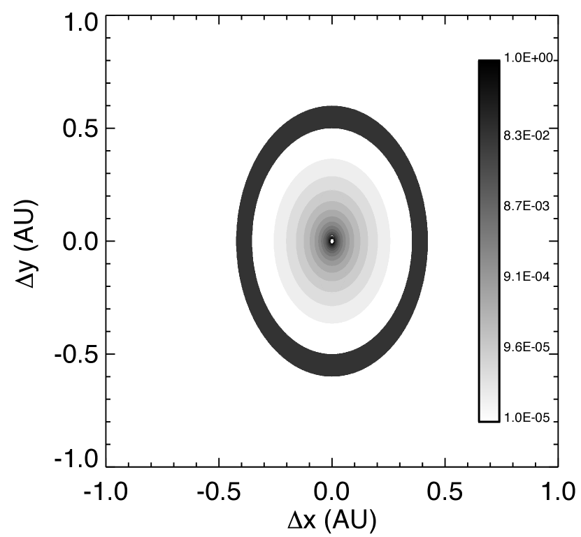
Figure 4: Synthetic, velocity-integrated image, computed for the disk model described in §3.1 assuming $R_{\rm ring}=0.5$ AU, $R_{\rm in}=0.01$ AU, PA=0, $i=45^{\circ}$, $\alpha=3$, a line-to-continuum ratio of 0.5, and $M_{\ast}=3$ M_⊙. The image has been normalized, and is shown with a logarithmic stretch. Note that the star is not included in this synthetic image.

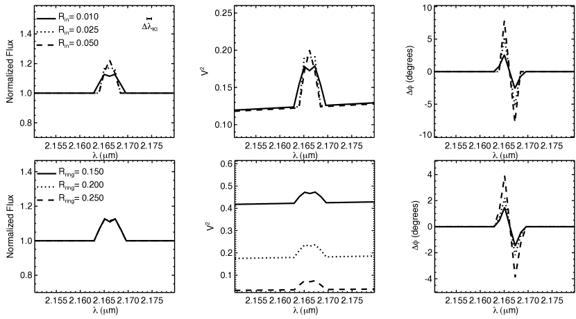
Figure 5: Synthetic fluxes, $V^{2}$, and differential phases ($\Delta\phi$) computed for the disk model described in §3.1. We assume a fiducial model with $R_{\rm in}=0.01$ AU, PA=0, $i=45^{\circ}$, $\alpha=3$, a line-to-continuum ratio of 0.5, $d=140$ pc, and $M_{\ast}=3$ M_⊙. Here, we vary $R_{\rm in}$ (top) and $R_{\rm ring}$ (bottom), and illustrate the effects of these variations on the synthetic data.

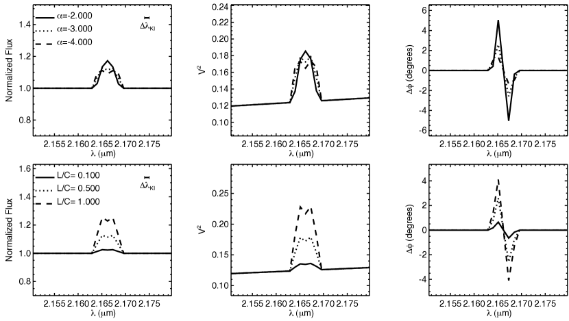
Figure 6: Synthetic fluxes, $V^{2}$, and differential phases ($\Delta\phi$) computed for the disk model described in §3.1. Assuming the fiducial model described in Figure 5, we vary $\alpha$ (top) and $L/C$ (bottom) and illustrate the effects of changing these parameters on the synthetic data.

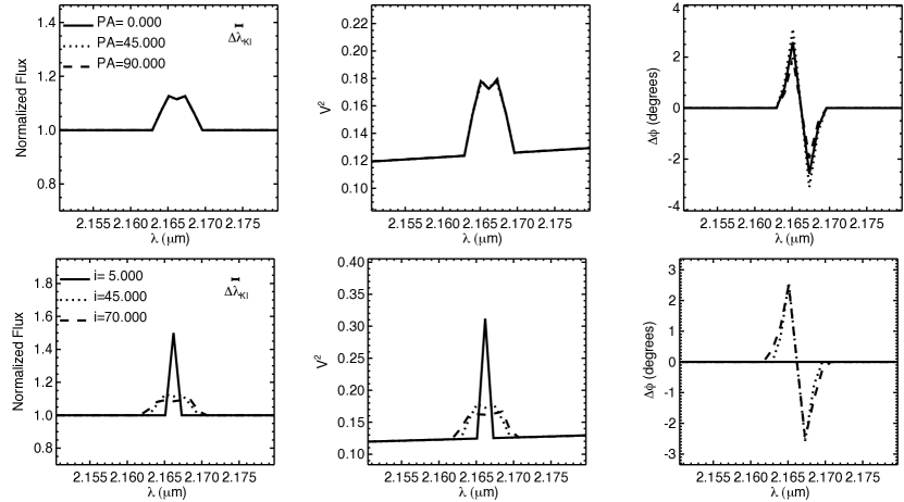
Figure 7: Synthetic fluxes, $V^{2}$, and differential phases ($\Delta\phi$) computed for the disk model described in §3.1. Assuming the fiducial model described in Figure 5, we vary $PA$ (top) and $i$ (bottom) and illustrate the effects of changing these parameters on the synthetic data.

An image of an example disk model is shown in Figure 4. Different disk morphologies can be obtained by adjusting the free parameters described above. These parameters can be considered in three groups: disk geometry, described by $R_{\rm in}$ and $R_{\rm ring}$; the disk brightness profile, parameterized by $\alpha$ and $L/C$; and the viewing geometry, described by $PA$ and $i$. Before describing the results of fitting these disk models to data, we start with brief discussion of how model parameters affect synthetic fluxes, $V^{2}$, and differential phases. These effects are illustrated in Figures 5–7, and described in the following sections.

3.1.1 Disk Geometry

Here we consider the effects of $R_{\rm in}$ and $R_{\rm ring}$ on fluxes, $V^{2}$, and differential phases predicted by disk models. A smaller value of $R_{\rm in}$ means that while there is emission from smaller radii, there will also be less emission from gas at larger radii (for a given line-to-continuum ratio). Thus the line profile becomes broader as more flux is distributed to the higher-velocity material at small radii. The system becomes less spatially resolved at these high velocities (i.e., in the line wings), since the $L/C$ of the compact emission has increased. The emission becomes more resolved for lower velocities as the $L/C$ of this emission decreases (and the mean size thus shifts out toward the continuum ring). Smaller values of $R_{\rm in}$ drive centroid offsets closer to zero, and hence lead to smaller $\Delta\phi$.

Values of $R_{\rm in}$ larger than those shown in Figure 5 lead to even narrower profiles of flux and $V^{2}$ versus wavelength, and larger differential phase signatures. For very large $R_{\rm in}$, the line may become completely spectrally unresolved, in which case the $\Delta\phi$ would become zero. Since observed spectra for all targets show spectrally resolve Br$\gamma$ line profiles (Figure 1), we do not consider values of $R_{\rm in}$ larger than 0.05 AU in this modeling.

Because $R_{\rm ring}$ is also taken to be the outer radius of the gaseous disk, it does have an impact on the observables beyond the normalization of the continuum. Larger values of $R_{\rm ring}$ lead to larger centroid offsets between the red and blue sides of the gaseous disk. Moreover, larger values of $R_{\rm ring}$ lead to a lower correlated continuum flux ($V_{\rm cont}F_{\rm cont}$), meaning that the contribution of the symmetric continuum component to the total measured differential phase signal is decreased (see Equation 6). Thus, a larger radius of the continuum emission helps to amplify any differential phase signal arising from the gaseous emission. Note that $R_{\rm ring}$ is determined directly from a fit of a ring model to continuum data, and so is not actually a free parameter in the models.

3.1.2 Disk Brightness Profile

The disk brightness profile depends on the line-to-continuum ratio ($L/C$), which determines the normalization, and on $\alpha$, which describes the radial profile. Both have prominent effects on the synthetic data (Figure 6).

Steeper brightness profiles, corresponding to higher values of $\alpha$, result in a higher proportion of flux in the extreme velocities. Hence large values of $\alpha$ result in double-peaked profiles, while $\alpha$ values closer to zero result in single-peaked profiles. Models with shallower flux profiles will be more spatially resolved, since more flux is found at larger radii. Similarly, differential phases deviate from zero more strongly for shallower flux profiles. Note that the effects of increasing $\alpha$ are similar to the effects of decreasing $R_{\rm in}$.

Higher line-to-continuum ratios produce brighter lines in model spectra (by definition). Because of the higher proportion of flux in the compact gaseous component relative to the continuum ring, models with higher line-to-continuum ratios also produce less resolved (higher) $V^{2}$ within the emission line. Higher line-to-continuum ratios mean that the centroid offsets between different velocity components of the gaseous disk have less dilution from the continuum ring (which has no centroid offset versus wavelength). Thus we find larger differential phase signatures for higher line-to-continuum ratios.

3.1.3 Disk Viewing Geometry

The position angle has no effect on the total flux emitted, although it may impact the modeled $V^{2}$ and $\Delta\phi$, since models (and data) are only “observed” over a limited range of baseline position angles. If the baseline PA is aligned with the disk PA, then the system will appear more resolved, and differential phase signals will be larger. If the baseline PA is orthogonal to the disk PA, the system will be less resolved, and we will observe no differential phase deviations from zero.

Face-on disks show no radial velocity gradients, and near-to-face-on disks show narrow emission features. For sufficiently low inclinations, all of the disk emission fits into a single spectral channel in our synthetic spectra. While the emission in this channel will be more compact (higher $V^{2}$) than the surrounding continuum, such a model produces no differential phase signature since the average centroid offset of the entire disk is zero. In contrast, higher inclinations mean broader emission lines, which lead to $V^{2}$ and $\Delta\phi$ signatures in multiple channels. The magnitude of these signatures depends on whether the disk PA is aligned with the baseline PA, and on the inclination. In Figure 7, the gaseous disk becomes less resolved with increasing inclination, since the system PA is not perfectly aligned with the baseline PA.

With a single baseline, we do not claim that we can constrain the position angle or inclination of the disk. However, we allow these parameters to vary in the models to reflect potential misalignments between the baseline $PA$ and the disk.

3.2 Magnetospheric Infall/Outflow Models

We also consider models that include gaseous outflows or inflows interior to the dust sublimation front. We allow these outflows to extend to scales larger than the dust sublimation radii. As with the disk model considered in §3.1, we include a ring of continuum emission. For simplicity here, we assume the position angle and inclination of the ring are zero. Note that the ring geometry is not coupled to the morphology of the gas.

We assume an infall/outflow cone with an opening angle of $5^{\circ}$. The cone has a position angle, $PA$, and an inclination with respect to the plane of the sky, $\phi$. We allow the infall/outflow to extend from an outer radius, $R_{\rm out}$ to an inner radius, $R_{\rm in}$. In contrast to the disk model considered above, $R_{\rm out}\neq R_{\rm ring}$ here.

The velocity of material in this cone is described as a radial power-law:

$$v_{\rm obs}(R)=v_{\rm in}\left(\frac{R}{R_{\rm in}}\right)^{-\beta}\sin\phi.$$ (13)

Here, the velocity of material at the inner edge of the infall/outflow structure, $v_{\rm in}$, is chosen to produce a specified linewidth of the emission,

$$\Delta v=v_{\rm in}\sin\phi.$$ (14)

Examination of Equations 13 and 14 shows that the velocity profile depends on $\Delta v$, $R_{\rm in}$, and $\beta$, but not directly on $\phi$. The geometry of the outflow of the sky depends on $PA$, as well as on $R_{\rm in}$ and $R_{\rm out}$, but again not explicitly on $\phi$. We thus fix $\phi=45^{\circ}$ in our models.

We include another cone, reflected through the origin, with the same velocity profile multiplied by $-1$. Thus, the model includes a bipolar infall/outflow structure within the dust sublimation radius.

The brightness distribution of the infall/outflow cones is

$$B_{\rm infall/outflow}(R)=B_{\rm in}\left(\frac{R}{R_{\rm in}}\right)^{-\alpha},$$ (15)

where $B_{\rm in}$ is chosen to reproduce a specified line-to-continuum ratio. As above, $L/C$ is defined as the total, integrated flux of the gaseous emission over the total flux of the continuum. Note that $\alpha$ rolls all information about the temperature and surface density profile of the infall/outflow structure into a single parameter. Finally, we include as a free parameter a factor by which the flux in one of the two cones or “poles” or the infall/outflow may be scaled. We denote this factor as $f_{\rm a}$, since it represents an asymmetry in the model.

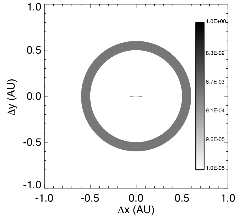
Figure 8: Synthetic, velocity-integrated image, computed for the infall/outflow model described in §3.2 assuming $R_{\rm in}=0.01$ AU, $R_{\rm out}=0.1$ AU, $PA=0$, $\alpha=2$, $\beta=2$, $\Delta v=250$ km s^-1, $L/C=0.5$, and $f_{\rm a}=0.5$. The image has been normalized, and is shown with a logarithmic stretch. Note that the star is not included in this synthetic image.

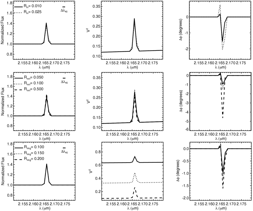
Figure 9: Synthetic fluxes, $V^{2}$, and differential phases ($\Delta\phi$) computed for the infall/outflow model described in §3.2. The fiducial model assumes $R_{\rm in}=0.01$ AU, $R_{\rm out}=0.1$ AU, $PA=0$, $\alpha=2$, $\beta=2$, $\Delta v=250$ km s^-1, $L/C=0.5$, $f_{\rm a}=0.5$, and $d=140$ pc. Here we vary $R_{\rm in}$, $R_{\rm out}$, and $R_{\rm ring}$ to demonstrate the effects of these parameters on the synthetic data. Note, however, that $R_{\rm ring}$ is not actually a free parameter in our infall/outflow models.

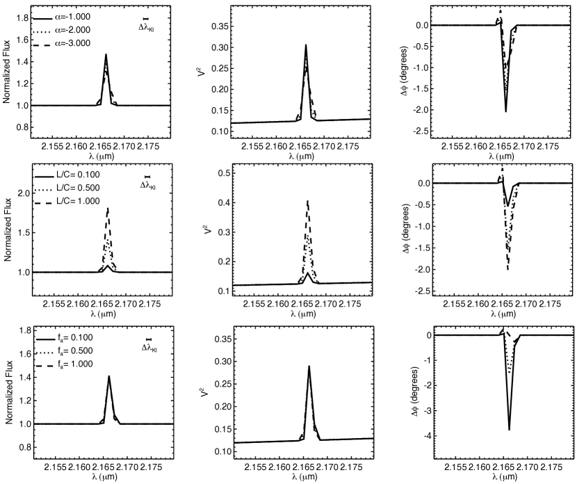
Figure 10: Synthetic fluxes, $V^{2}$, and differential phases ($\Delta\phi$) computed for the infall/outflow model described in §3.2. The fiducial model is as described in Figure 9, and we vary $\alpha$, $L/C$, and $f_{\rm a}$ here.

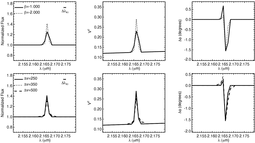
Figure 11: Synthetic fluxes, $V^{2}$, and differential phases ($\Delta\phi$) computed for the infall/outflow model described in §3.2. The fiducial model is as described in Figure 9, and we vary $\beta$ and $\Delta v$ here.

An image of an example infall/outflow model is shown in Figure 8. Different models may be generated by varying the free parameters $R_{\rm in}$, $R_{\rm out}$, $PA$, $\alpha$, $\beta$, $\Delta v$, $L/C$, and $f_{\rm a}$. We now summarize the effects of each of these parameters on synthetic fluxes, $V^{2}$, and differential phases, and illustrate these effects in Figures 9–12.

3.2.1 Infall/Outflow Geometry

The inner and outer radii of the infall/outflow structure have small effects on modeled fluxes and $V^{2}$, but can have a larger effect on the differential phases. The larger effects on $\Delta\phi$ stem from the greater sensitivity of differential phases to compact structure. Since centroiding accuracy is better than the angular resolution (by a factor of the S/N), smaller source structure can be constrained.

A larger inner radius means that the highest-velocity material is located farther from the star, and so covers more area. The relative amount of flux in the high-velocity component of the outflow is thus increased, which leads to a flatter line profile. Since the line-to-continuum ratio is increased for high velocity material, but decreased for low-velocity gas, the $V^{2}$ versus wavelength also flattens. Larger values of $R_{\rm in}$ drive larger centroid offsets, and hence lead to larger $\Delta\phi$. Similarly, larger values of $R_{\rm out}$ lead to (somewhat) more extended emission, and hence to larger centroid offsets.

As for the disk model considered above, a larger value of $R_{\rm ring}$ leads to less correlated flux from the continuum component. This decreases the contribution of the continuum to the observed differential phases, and will amplify any differential phase signatures coming from the infall/outflow component.

3.2.2 Infall/Outflow Brightness Profile

The effect of $\alpha$ on the observables is similar to the effects described above in the context of disk models. The line profile becomes less peaked, the $V^{2}$ versus wavelength also become less peaked, and the differential phase signatures get smaller as the brightness profile of the model is steepened. The dependence of the synthetic data on $L/C$ for the infall/outflow model is the same as for the disk model described above.

Decreasing $f_{\rm a}$ increases the flux ratio between the blue and red sides of the infall/outflow structure. This manifests itself through slight asymmetries in the synthetic flux and $V^{2}$ versus wavelength. The effect on synthetic differential phases is more pronounced, since these are more sensitive to the differences in emission on such compact scales.

3.2.3 Infall/Outflow Velocity Structure

The effect of $\beta$ on the observables similar to, but not degenerate with, the effects of $\alpha$. A steeper velocity profile means that more of the low-velocity gas is found at smaller stellocentric radii, where the emission is stronger. Thus, a higher value of $\beta$ is similar to a smaller value of $\alpha$. However, comparison of this Figures 10 and 11 demonstrates that the effects on the synthetic data are sufficiently different so as to be distinguishable.

As $\Delta v$ is increased the line profile becomes broader and flatter (flatter because the line-to-continuum ratio is held fixed for a given parameter study). The $V^{2}$ versus wavelength also becomes broader and flatter. Examination of Equations 13 and 14 shows that the physical effect of increasing $\Delta v$ is to increase the radial velocity at the inner edge of the infall/outflow structure. This, in turn, causes the radius where the infall/outflow reaches systemic velocity to move outward. A larger offset of the near-zero velocity material leads to a larger differential phase signature.

3.2.4 Infall/Outflow Viewing Geometry

The effect of $PA$ on the observables is similar to the effects described above in the context of disk models. Since the differential phases are sensitive to structure on smaller scales than the $V^{2}$, and the infall/outflow model generates most of its flux on compact scales, it is not surprising the $\Delta\phi$ is more sensitive than $V^{2}$ to $PA$ changes. For the definition of our model, $\phi$ has no direct effect on the synthetic data.

3.3 Model Fitting

We compute grids of models using the parameter values shown in Figures 5–12. Grids with more finely-sampled parameter values are not possible given the computational time needed to compute these models. Our disk model grid requires 1–2 weeks, while our infall/outflow model grid (which has more free parameters) requires over 3 weeks to run on a fast desktop computer.

After computing synthetic fluxes, $V^{2}$, and $\Delta\phi$ values for grids of both disk and infall/outflow models, we compute the reduced $\chi^{2}$ residuals between these and the observed quantities. The total $\chi^{2}$ is given by

$$\chi^{2}_{\rm tot}=\sqrt{(\chi^{2}_{\rm flux})^{2}+(\chi^{2}_{\rm V^{2}})^{2}+(\chi^{2}_{\rm\Delta\phi})^{2}}.$$ (16)

Finally, we minimize $\chi^{2}_{\rm tot}$ to determine the “best-fit” model. With such a sparse grid of models, we can not claim that our “best-fit” model is the true, absolute minimum of the $\chi^{2}$ surface, as opposed to a deep local minimum. Furthermore, we can not give rigorous error intervals on the fitted parameters, since we have not adequately sampled the $\chi^{2}$ surface.

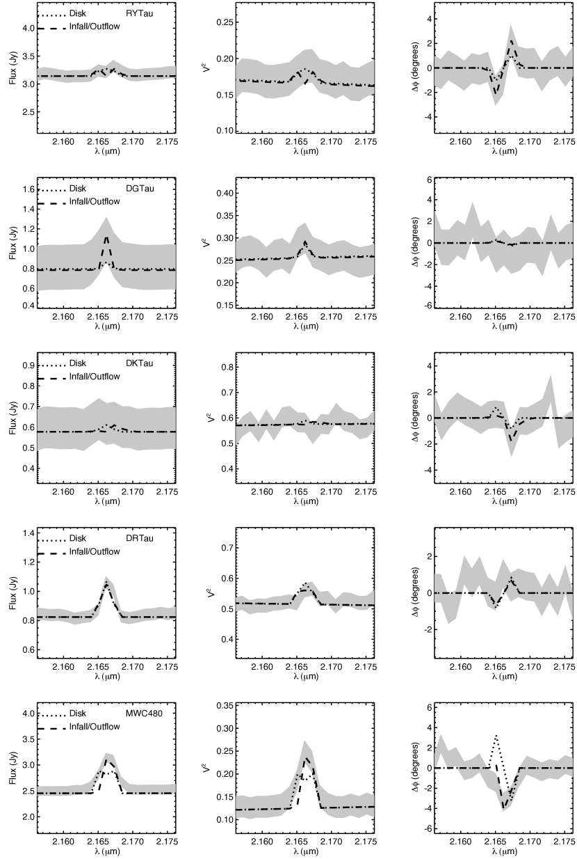
Figure 13: Observed fluxes, $V^{2}$, and $\Delta\phi$ values (gray regions indicate 1-$\sigma$ confidence intervals), and synthetic data for best-fit disk (dotted curves) and infall/outflow (dashed curves) models.

The best-fit models are illustrated in Figure 13. Reduced $\chi^{2}$ values, and parameters of the best-fitting models, are listed in Table 4.

4 Results and Analysis

4.1 Accretion properties inferred from Br$\gamma$ Spectra

Before discussing the distribution of circumstellar matter for our sample, we begin by analyzing our Br$\gamma$ spectra and estimating accretion luminosities using tools that have been developed and used previously. These accretion luminosities will provide some basis for comparison against the circumstellar properties.

In Table 5 we list the equivalent widths (EWs) of the Br$\gamma$ lines measured for our sample, after removal of the stellar components of the spectra using the procedure described in §2.7. Following Eisner et al. (2007c), we use these equivalent widths in conjunction with literature photometry and extinction estimates to determine the Br$\gamma$ line luminosities.

These line luminosities are then converted into accretion luminosities using an empirically-determined relationship from Muzerolle et al. (1998, 2001). This relationship is determined by comparing Br$\gamma$ line luminosities to accretion luminosities determined by fitting shock models to UV data. Note, however, that this relationship was determined for mostly solar-type T Tauri stars. While the relationship has been extended to $\sim 3$ M_⊙ stars (Calvet et al. 2004), it has not been calibrated at high stellar masses and may break down for targets like MWC 1080. In fact, we argue below and elsewhere (e.g., Eisner et al. 2004) that this object may not undergo magnetospheric accretion, in which case the relationship from Muzerolle et al. (1998, 2001) is almost certainly invalid.

The accretion luminosity can be converted into an accretion rate: $\dot{M}\approx L_{\rm acc}R_{\ast}/GM_{\ast}$. Since Br$\gamma$ is in absorption for V1057 Cyg, neither $L_{\rm acc}$ nor $\dot{M}$ is meaningful in this case. For AS 353 and V1331 Cyg, we do not have reliable estimates of stellar parameters, and so we can not estimate $\dot{M}$.

Table 5 shows that our sample spans a wide range in Br$\gamma$ luminosity, and hence in accretion luminosity and mass accretion rate. Measured EWs (and accretion luminosities and mass accretion rates) are generally within a factor of two of previous measurements (Najita et al. 1996; Folha & Emerson 2001; Calvet et al. 2004; Eisner et al. 2007c). Given the large variations in Br$\gamma$ EW over multiple epochs observed by previous investigators (e.g., Najita et al. 1996; Eisner et al. 2007c), our measurements seem compatible with the previous results.

4.2 Distribution of Br$\gamma$ Emission

For many objects in our sample, both the disk and infall/outflow models considered above provide reasonable fits to the data (Table 4), and so we can not distinguish between the two models, at least based on the available data. However, there are several sources for which we can distinguish. For MWC 480, MWC 863, and MWC 275, the $\chi_{r}^{2}$ values for fits of the disk model are substantially higher than those of infall/outflow model fits. These objects all show strong Br$\gamma$ emission, and have been observed at high S/N. It seems likely that higher S/N observations of some fainter targets in our sample–especially those exhibiting bright Br$\gamma$ emission–would also show them to be better described by infall/outflow models.

To understand why the data for these objects are fitted better by infall/outflow models, consider the following argument. If the Br$\gamma$ line is spectrally resolved–which is easiest to determine for bright objects with strong emission–then one expects to see differential phase signatures as long as the gaseous emission is not very compact. If the gas is very compact, this leads to double-peaked line profiles for disk models, contradicting the observations. To ensure single-peaked line profiles, the brightness profiles of disk models must be shallow. However, this produces differential phase signals larger than observed. Infall/outflow models, on the other hand, can produce single-peaked line profiles without large centroid offsets. For example, if one posits an infall pointed nearly toward the observer, a lot of flux could come from near-systemic velocities without creating a large centroid offset (on the sky) of different velocity components.

For fainter sources, it is difficult to apply this argument, because of the lower signal-to-noise in both flux and differential phase measurements. Noisier fluxes make it harder to rule out models predicting spectrally unresolved emission (which also predict no $\Delta\phi$ signature), while noisy $\Delta\phi$ measurements make it harder to rule out large centroid offsets with wavelength of the model emission. However, it is likely that observations of (some of) these fainter sources with higher S/N would find a preference for infall/outflow models .

We note that the orientation of the KI baseline with respect to the disk position angle can be estimated in a few cases. For MWC 275, MWC 480, and MWC 758, estimated disk PAs (Tannirkulam et al. 2008; Eisner et al. 2004) are nearly orthogonal to the baseline PA. This supports our interpretation of the data for MWC 480 and MWC 275 in terms of outflow models. In contrast, for MWC 1080, the estimated disk PA (Eisner et al. 2004) is nearly aligned with the KI baseline, suggesting that the Br$\gamma$ observations may be sensitive to rotating gas in this source.

5 Discussion

5.1 Br$\gamma$ as a Tracer of Magnetospheric Accretion

In §4.2, we argued that the spectra, $V^{2}$, and differential phases measured for our sample are more compatible with infall/outflow models than with disk models, at least in some cases. Somewhat less direct evidence also argues against disk models for some of our targets. Low-mass young stars are thought to accrete material not via a boundary layer between star and accretion disk, but rather through funnel flows originating near the magnetospheric radius and then following stellar magnetic field lines to high-latitude regions of the star (e.g., Königl 1991; Hartmann 1998). This magnetospheric accretion picture provides a natural mechanism for truncating circumstellar disks and hence allowing direct illumination of the inner edge. This, in turn, would lead to the puffed-up inner disk walls evinced by continuum measurements of the inner regions of disks around T Tauri and Herbig Ae stars (Millan-Gabet et al. 2007, and references therein).

While our data are often fitted better with infall/outflow models, we can not distinguish between infall and outflow models directly with the spatial and kinematic constraints provided by our observations. However, we can compare our results with size scales of gaseous emission predicted by various physical infall or outflow models. Matter falling in along stellar magnetic field lines will glow brightly near to the stellar surface, where it converts most of its gravitational potential energy to radiation, and so we would expect to see Br$\gamma$ emission from very close to the stellar surface in this case (e.g., Muzerolle et al. 1998). For models where the Br$\gamma$ emission arises in hot, magnetically-launched winds, we might see emission close to the magnetospheric radius at hundredths to tenths of an AU (as in the X-wind model; e.g., Shu et al. 1994) or in the range of an AU or more (as in the disk-wind model; e.g., Konigl & Pudritz 2000).

Our modeling suggests that the Br$\gamma$ emission in most objects arises in material that extends very close to the central star ($\lesssim 0.01$ AU; Table 4), consistent with expectations of magnetospheric infall models. This conclusion is supported for most sources by the very small average sizes of the Br$\gamma$ emission found from simple geometric fits to the data (Table 3).

However, for some targets, we infer somewhat larger inner radii and/or shallow brightness profiles for the Br$\gamma$ emission. Somewhat larger sizes are also inferred for the average Br$\gamma$ emission from these targets ($\sim 0.05$–0.2 AU; Table 3). Evidently, much of the Br$\gamma$ emission from these objects is found on scales larger than expected from accretion columns. X-wind or disk wind models predict more Br$\gamma$ emission from larger radii, potentially consistent with the inferred size scales and brightness profiles for these sources.

Based on these arguments it seems likely that in the sample of objects with steeper brightness profiles, Br$\gamma$ emission traces magnetospheric accretion. For sources with shallower brightness profiles, Br$\gamma$ emission traces: infalling material that has a shallow radial brightness profile; outflowing material that is magnetospherically launched from small radii; or a combination of both infalling and outflowing material. In the latter case, the infalling material could produce very compact emission while more extended winds could “fill in” the emission profile as larger radii.

Further support for magnetospheric accretion as the origin for (some of) the Br$\gamma$ emission comes from analysis of line profiles observed at higher spectral (but lower spatial) resolution. While most of our targets exhibit H$\alpha$ emission showing P Cygni profiles of winds (e.g., Acke et al. 2005; Najita et al. 1996, and references therein), the Br$\gamma$ line profiles are more symmetric and/or blueshifted, and often show a “blue shoulder” (Najita et al. 1996; Folha & Emerson 2001; Eisner et al. 2007c). These properties are all consistent with infalling material rather than winds (Najita et al. 1996).

5.2 Trends with Stellar Properties

While magnetospheric accretion is favored for low-mass stars, previous investigators have argued that disk accretion may be a better description in Herbig Be stars (e.g., Eisner et al. 2004). Thus, for MWC 1080, the one Herbig Be star in our sample, one might expect the disk model considered above to fit the data well. Note that the gaseous disk described in §3.1 could correspond physically to the inner accretion disk expected for a boundary layer accretion scenario where disk material in Keplerian rotation shocks when it hits the slower-rotating stellar equator (e.g., Lynden-Bell & Pringle 1974).

Disk models fit the data for this source approximately as well as outflow models. Furthermore, the orientation of the KI baseline along the disk major axis lends credence to the hypothesis that the Br$\gamma$ we observe traces disk rotation. Thus, our current study supports the idea that Herbig Be stars may accrete material through geometrically thin disks rather than magnetospheric accretion columns.

5.3 Trends with Br$\gamma$ Line Luminosities

Our sample clearly exhibits a range in Br$\gamma$ line-strength (Figure 1), which correlates with Br$\gamma$ line luminosity and accretion luminosity (Table 5). We are thus in a position to explore whether the circumstellar properties of the Br$\gamma$ emission depend on the overall strength of the emission.

Beyond stronger line-to-continuum ratios, it is unclear what we would expect the effects of stronger Br$\gamma$ emission (and by extension accretion luminosity or rate) to be on the observed data and models. If Br$\gamma$ emission strength was correlated with the emission morphology–e.g., if stronger Br$\gamma$ emission tended to trace infall while weaker emission traced outflow from larger stellocentric radii–then we might expect trends in the data.

The simplest way to search for trends is to look at inferred size of the Br$\gamma$ emission versus the accretion luminosity. Figure 16 shows no obvious correlation between the two. Similarly, a comparison of Tables 4 and 5 shows no clear correlation between $L_{\rm Br\gamma}$ and $\alpha$. Thus, there is no strong indication that Br$\gamma$ emission strength determines the overall morphology.

We do, however, see some (inverse) correlation between the inferred inner radius of the Br$\gamma$ emission and the accretion luminosity. Considering best-fit parameters for infall/outflow model fits, and excluding MWC 1080, which appears to be fitted better with a disk model, we plot the inner radius of the infall/outflow inferred from our modeling against $L_{\rm acc}$ in Figure 17. This may indicate that sources that convert more gravitational energy into Br$\gamma$ luminosity do so at preferentially smaller stellocentric radii. For example, sources where Br$\gamma$ traces accreting flows will exhibit the most compact emission, and may also produce higher Br$\gamma$ luminosities. Alternatively, the trend seen in Figure 17 could fit in with an X-wind scenario where Br$\gamma$ emission traces the innermost regions of an outflow: higher accretion rates–which mean more gravitational energy release–push the “X-point” to smaller stellocentric radii as accretion pressure pushes in against stellar magnetic pressure.

5.4 Comparison with previous results

As discussed in the introduction, Kraus et al. (2008) observed five Herbig Ae/Be sources with the VLTI interferometer, and obtained spatially and spectrally resolved data indicating that the Br$\gamma$ emission arose on scales larger than expected for magnetospheric accretion models. Their derived sizes of the gaseous emission were a few tenths of an AU for the Herbig Ae sources and a few AU for the Herbig Be objects.

Fitting ring models to the Br$\gamma$ emission, as done by Kraus et al. (2008), we typically find substantially smaller sizes (Table 3). For MWC 275, the size we infer for the Br$\gamma$ emission is $\sim 10$ times smaller than that found by Kraus et al. (2008). We note that the components of the MWC 275 visibilities attributed to Br$\gamma$ by Kraus et al. (2008) are all consistent with unity, and we would therefore argue that their data are consistent with the compact size for this object determined here. Given the greater angular resolution of KI relative to VLTI, we are more sensitive to emission on compact scales, and so it is not overly surprising that we are able to better constrain Br$\gamma$ emission at small stellocentric radii.

The modeling presented here suggests emission over a range of radii. While some objects have average Br$\gamma$ emission sizes as large as $\sim 0.1$ AU (Table 3), the combination of spectrally resolved flux and $V^{2}$ profiles and small differential phases for these targets indicates some Br$\gamma$-emitting gas on $\sim 0.01$ scales (Table 4). Thus, all of our targets where Br$\gamma$ emission is observed appear to have some gas on very compact scales.

While Kraus et al. (2008) argued that the Br$\gamma$ emission appeared to trace more extended disk winds, our results and modeling belie this conclusion. Rather, we suggest that the Br$\gamma$ emission traces accreting material in many, if not most, sources. In others, Br$\gamma$ emission may trace a combination of accretion and outflow, or perhaps compact ($\lesssim 0.05$ AU) wind-launching regions.

6 Conclusions and Future Work

We presented observations capable of resolving hydrogen gas on scales as small as 0.01 AU around young stars. These were the first such observations of solar-type T Tauri stars, and extended the mass range and sample size of previous studies at similar spectral (but somewhat lesser spatial) resolution.

We showed that Br$\gamma$ emission is typically more compactly distributed than the continuum emission around young stars. In several objects, the bulk of the Br$\gamma$ emission is found on scales $\lesssim 0.01$ AU. In others, the average size of the Br$\gamma$ emission is $\sim 0.1$ AU, although modeling of our combined dataset shows evidence for some Br$\gamma$ emission extending in to within a few hundredths of an AU of the central stars. For sources with very small average sizes of the Br$\gamma$ emission, an origin of the Br$\gamma$ emission in accretion flows appears to be the best explanation. For objects with somewhat more extended Br$\gamma$ distributions, the emission probably traces the innermost regions of magnetospherically launched winds, or perhaps some combination of infall and outflow.

No obvious trends are seen in the average size of the Br$\gamma$ emission versus accretion luminosity. However, there appears to be some inverse correlation between the inner radius for our best-fit models and the Br$\gamma$ emission strength. Such a correlation may indicate a relationship between the physical origin of the Br$\gamma$ emission and its luminosity.

While all of our observations are compatible with infall/outflow models, the data for the most massive star in our sample, MWC 1080, appear equally consistent with a Keplerian disk model. Previous investigators have argued that this object may have a dense, gaseous, inner disk that prevents direct stellar irradiation of dust near the sublimation radius. Our modeling of this source is consistent with a disk origin of the Br$\gamma$ emission.

While we observed V1057 Cyg, we did not discuss it at length here. V1057 Cyg is the one target in our sample where Br$\gamma$ appears in absorption, rather than emission. As an FU Ori star, the luminosity of this source is dominated by accretion energy released in the disk midplane (e.g., Hartmann et al. 2004), and so most lines should appear in absorption (e.g., Calvet et al. 1991). We plan to discuss this source in detail in a future paper targeting FU Ori sources.

We also plan to extend the analysis presented above to other spectral regions. Although we focused on Br$\gamma$ here, our experimental setup included the CO overtone bandheads as well as regions of significant opacity from water vapor. In fact, several objects discussed here also show interesting spectral features in the region of the CO bandheads. Because the currently observed $V^{2}$ and $\Delta\phi$ signatures associated with these features are marginal, we postpone discussion to future work, when we hope to have higher S/N data.

Data presented herein were obtained at the W. M. Keck Observatory, from telescope time allocated to the National Aeronautics and Space Administration through the agency’s scientific partnership with the California Institute of Technology and the University of California. The Observatory was made possible by the generous financial support of the W. M. Keck Foundation. The authors wish to recognize and acknowledge the cultural role and reverence that the summit of Mauna Kea has always had within the indigenous Hawaiian community. We are most fortunate to have the opportunity to conduct observations from this mountain. The ASTRA program, which enabled the observations presented here, was made possible by funding from the NSF MRI grant AST-0619965. This work has used software from NExSci at the California Institute of Technology. The Keck Interferometer is funded by the National Aeronautics and Space Administration as part of its Exoplanet Exploration program.

Table 1: Target and Calibrator Properties

Source	$\alpha$	$\delta$	$d$	Spectral Type	$m_{V}$	$m_{K}$	References
	(J2000)	(J2000)	(pc)
Target Stars
RY Tau	04 21 57.409	+28 26 35.56	140	K1	10.2	5.4	1
DG Tau	04 27 04.700	+26 06 16.20	140	K3	12.4	7.0	2
DK Tau A	04 30 44.28	+26 01 24.6	140	K9	12.6	7.1	3
DR Tau	04 47 06.21	+16 58 42.8	140	K4	13.6	6.9	2
MWC 480	04 58 46.266	+29 50 37.00	140	A2	7.7	5.5	4
RW Aur A	05 07 49.568	+30 24 05.161	140	K2	10.5	7.0	2
MWC 758	05 30 27.530	+25 19 57.08	140	A3	8.3	5.8	4
AS 205 A	16 11 31.402	-18 38 24.54	160	K5	12.1	6.0	6
MWC 863 A	16 40 17.922	-23 53 45.18	150	A2	8.9	5.5	5
V2508 Oph	16 48 45.62	-14 16 35.9	160	K6	13.5	7.0	6
MWC 275	17 56 21.288	-21 57 21.88	122	A1	6.9	4.8	5
AS 353 A	19 20 30.992	+11 01 54.550	150	F8	12.5	8.4	7
V1057 Cyg	20 58 53.73	+44 15 28.54	600	G5	11.7	6.2	8
V1331 Cyg	21 01 09.21	+50 21 44.8	700	G5	11.8	8.6	9
MWC 1080	23 17 25.574	+60 50 43.34	1000	B0	11.6	4.7	4
Calibrator Stars							Applied to:
HD23642	03 47 29.453	+24 17 18.04	110	A0V	6.8	6.8	DG Tau,DK Tau A,DR Tau,RW Aur A
HD23632	03 47 20.969	+23 48 12.05	120	A1V	7.0	7.0	DG Tau,DK Tau A,DR Tau,RW Aur A
HD 23753	03 48 20.816	+23 25 16.499	104	B8V	5.4	5.7	RY Tau,MWC 480,MWC 758
HD 27777	04 24 29.155	+34 07 50.73	187	B8V	5.7	6.0	RY Tau,MWC 480,MWC 758
HD31464	04 57 06.426	+24 45 07.90	45	G5V	8.6	7.0	DG Tau,DK Tau A,DR Tau,RW Aur A
HD139364	15 38 25.358	-19 54 47.45	53	F3V	6.7	5.7	AS 205 A
HD141465	15 49 52.297	-17 54 07.007	43	F3V	6.8	5.9	AS 205 A
HD144821	16 08 16.582	-13 46 08.582	76	G2V	7.5	6.0	AS 205 A,V2508 Oph
HD148968	16 32 08.085	-12 25 53.910	146	A0V	7.0	7.0	AS 205 A, V2508 Oph
HD 149013	16 32 38.133	-15 59 15.12	41	F8V	7.0	5.7	MWC 863
HD 163955	17 59 47.553	-23 48 58.08	134	B9V	4.7	4.9	MWC 275
HD 170657	18 31 18.960	-18 54 31.72	13	K1V	6.8	4.7	MWC 275
HD183442	19 29 30.077	+03 05 23.607		B7V	8.1	8.4	AS 353 A
HD192985	20 16 00.615	+45 34 46.291	35	F5V	5.9	4.8	V1057 Cyg
HD195050	20 27 34.258	+38 26 25.194	83	A3V	5.6	5.5	V1057 Cyg
HD198182	20 46 53.060	+47 06 41.502	185	A1V	7.8	7.8	V1331 Cyg
HD219623	23 16 42.303	+53 12 48.512	20	F7V	5.6	4.3	MWC 1080

References. — (1) Muzerolle et al. (2003); (2) White & Ghez (2001); (3) Monin et al. (1998); (4) Eisner et al. (2004); (5) Monnier et al. (2006); (6) Eisner et al. (2005); (7) Prato et al. (2003); (8) Herbig et al. (2003); (9) Eisner et al. (2007c). Calibrator star distances are based on Hipparcos parallax measurements (Perryman et al. 1997).

Table 2: Log of Observations

Source	Date	$u$ (m)	$v$ (m)
RY Tau	2008 Novemver 18	56,56,56,56,46,46,45	57,57,58,58,71,71,71
DG Tau	2008 November 17	55,55,56,56,47,47,30,30	51,51,54,54,70,70,77,77
DK Tau	2008 November 17	56,56	56,56
DR Tau	2008 November 17	56,56,41,40	60,61,72,72
	2008 Novemver 18	56,56,41,40	60,61,72,72
MWC 480	2008 Novemver 18	56,46,46	56,70,71
RW Aur	2008 November 17	56,56,56,56,55,33,32	55,55,58,58,59,77,78
	2008 Novemver 18	56,56,56,56,55,33,32	55,55,58,58,59,77,78
MWC 758	2008 Novemver 18	56,56	58,59
AS 205a	2009 July 15	32,32,31,53,53,53,51,50	45,45,45,54,54,53,52,52
MWC 863	2009 July 15	44,44	44,43
V2508 Oph	2008 April 25	35,34,31	50,50,49
MWC 275	2009 July 15	52,52,50,50,54,54,50,49	51,51,49,49,53,52,49,48
AS 353	2009 July 15	52	66
V1057 Cyg	2009 July 15	54,54,52,51,51,49,49	56,57,60,61,61,64,64
V1331 Cyg	2009 July 15	44,43,40,39	67,67,71,71
MWC 1080	2009 July 15	48,48,45,44	55,56,60,61

Table 3: Inferred sizes of Br$\gamma$ emission regions

Source	$\theta_{\rm Br\gamma}$ (mas)	$R_{\rm Br\gamma}$ (AU)	$\theta_{\rm continuum}$ (mas)	$R_{\rm cont}$ (AU)
RY Tau	$<$0.12	$<$0.01	2.63 $\pm$ 0.03	0.18 $\pm$ 0.01
DG Tau	1.85 $\pm$ 0.04	0.13 $\pm$ 0.01	2.44 $\pm$ 0.02	0.17 $\pm$ 0.01
DK Tau	1.26 $\pm$ 0.07	0.09 $\pm$ 0.01	1.63 $\pm$ 0.06	0.11 $\pm$ 0.01
DR Tau	0.68 $\pm$ 0.16	0.05 $\pm$ 0.01	1.72 $\pm$ 0.04	0.12 $\pm$ 0.01
MWC 480	$<$0.10	$<$0.01	2.75 $\pm$ 0.01	0.19 $\pm$ 0.01
RW Aur	$<$0.10	$<$0.01	1.39 $\pm$ 0.07	0.10 $\pm$ 0.01
MWC 758	$<$0.21	$<$0.02	2.36 $\pm$ 0.02	0.18 $\pm$ 0.01
AS 205 A	$<$0.21	$<$0.02	2.02 $\pm$ 0.07	0.16 $\pm$ 0.01
MWC 863	0.97 $\pm$ 0.19	0.07 $\pm$ 0.01	3.84 $\pm$ 0.01	0.29 $\pm$ 0.01
V2508 Oph	0.56 $\pm$ 0.42	0.04 $\pm$ 0.03	3.81 $\pm$ 0.02	0.30 $\pm$ 0.01
MWC 275	0.45 $\pm$ 0.40	0.03 $\pm$ 0.02	3.13 $\pm$ 0.02	0.19 $\pm$ 0.01
AS 353	1.68 $\pm$ 0.05	0.13 $\pm$ 0.01	1.36 $\pm$ 0.06	0.10 $\pm$ 0.01
V1057 Cyg	$<$5.00	$<$1.50	1.27 $\pm$ 0.07	0.38 $\pm$ 0.02
V1331 Cyg	0.80 $\pm$ 0.13	0.28 $\pm$ 0.05	0.86 $\pm$ 0.12	0.30 $\pm$ 0.04
MWC 1080	0.42 $\pm$ 0.44	0.21 $\pm$ 0.22	2.66 $\pm$ 0.03	1.33 $\pm$ 0.02

Note. — Angular ring diameters ($\theta$) are converted into linear ring radii using the distances listed in Table Spatially and Spectrally Resolved Hydrogen Gas within 0.1 AU of T Tauri and Herbig Ae/Be Stars.

Table 4: Results of Modeling

Source	$\chi_{r}^{2}$	$R_{\rm in}$	$PA$	$i$	$L/C$	$\alpha$	$\chi_{r}^{2}$	$R_{\rm in}$	$R_{\rm out}$	$PA$	$\beta$	$\Delta v$	$L/C$	$f_{\rm a}$	$\alpha$
		(AU)	(∘)	(∘)				(AU)	(AU)	(∘)		(km s-1)
	Disk Models						Infall/Outflow Models
RYTau	0.09	0.03	45	70	0.1	4	0.08	0.03	0.10	90	1	350	0.1	1.0	1
DGTau	0.14	0.05	0	45	0.1	3	0.14	0.01	0.50	0	1	350	0.5	1.0	1
DKTau	0.27	0.05	45	70	0.1	2	0.26	0.03	0.10	45	1	500	0.1	0.1	1
DRTau	0.39	0.01	90	45	0.5	2	0.40	0.01	0.50	45	2	250	0.5	1.0	3
MWC480	0.86	0.03	90	45	0.5	4	0.51	0.03	0.10	0	2	250	0.5	0.1	3
RWAur	0.59	0.01	45	5	0.1	4	0.62	0.01	0.10	0	2	250	0.1	1.0	1
MWC758	0.20	0.03	0	70	0.1	4	0.20	0.01	0.05	45	2	250	0.1	1.0	3
AS205A	0.52	0.05	0	45	0.1	4	0.54	0.03	0.10	0	2	350	0.1	1.0	2
MWC863	0.44	0.03	0	45	0.5	4	0.35	0.01	0.05	0	1	250	0.5	0.1	1
V2508Oph	0.72	0.05	45	5	0.5	2	0.76	0.01	0.50	0	2	250	0.5	1.0	1
MWC275	0.54	0.01	0	45	0.5	4	0.30	0.01	0.05	90	2	250	0.5	0.5	3
AS353	0.77	0.05	0	5	1.0	2	0.73	0.03	0.50	0	1	250	1.0	1.0	2
V1057Cyg	0.54	0.01	90	70	0.1	4	0.47	0.03	0.05	0	1	500	0.1	1.0	3
V1331Cyg	0.56	0.05	90	5	0.5	2	0.49	0.01	0.50	90	1	350	1.0	1.0	1
MWC1080	0.28	0.03	90	45	0.5	2	0.26	0.03	0.10	45	2	500	0.5	1.0	1

Table 5: Properties Derived from Br$\gamma$ Spectra

Source	EW (Å)	$L_{\rm Br\gamma}$/($10^{-4}$ L⊙)	$L_{\rm acc}$/L⊙	$L_{\rm acc}$/L∗	$\dot{M}/(10^{-8}{\rm\>M_{\odot}\>yr^{-1}})$
RYTau	-1.0	1.9	0.5	0.1	6.4
DGTau	-8.1	3.8	1.3	1.5	7.6
DKTau	-2.2	0.8	0.2	0.2	1.2
DRTau	-7.1	3.1	1.0	1.1	5.7
MWC480	-7.7	9.8	4.4	0.2	9.3
RWAur	-7.2	2.7	0.9	0.5	4.8
MWC758	-1.4	1.9	0.6	0.1	1.1
AS205A	-2.6	3.7	1.3	1.0	8.1
MWC863	-5.5	7.3	3.0	0.2	6.4
V2508Oph	-5.8	4.2	1.5	0.5	17.2
MWC275	-6.1	14.7	7.3	0.2	17.5
AS353	-12.6	1.5	0.4
V1057Cyg	0.9
V1331Cyg	-13.5	30.7	18.4
MWC1080	-5.1	1181.4	1824.8	0.1	4374.6

Figure 1: Spectra of our sample in the spectral region around Br$\gamma$. Observed fluxes are plotted with solid black histograms. Circumstellar fluxes, determined using the procedure described in §2.7, are shown with gray histograms. For AS 353, V1057 Cyg, and V1331 Cyg, we assume that all of the near-IR flux arises from the circumstellar environment. For clarity of presentation, we have not plotted the error bars associated with the circumstellar fluxes; the magnitudes of the uncertainties are indicated in the upper right corners. Dotted gray lines indicate the central (rest) wavelength of the Br$\gamma$ transition, 2.1662 $\mu$m.

Figure 12: Synthetic fluxes, $V^{2}$, and differential phases ($\Delta\phi$) computed for the infall/outflow model described in §3.2. The fiducial model is as described in Figure 9, and we vary $PA$ here.

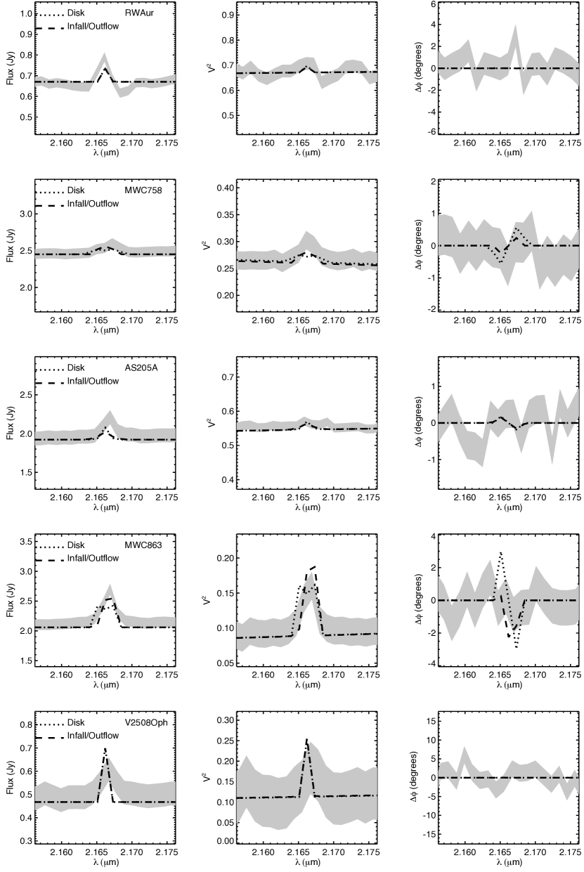
Figure 14: Figure 13 continued.

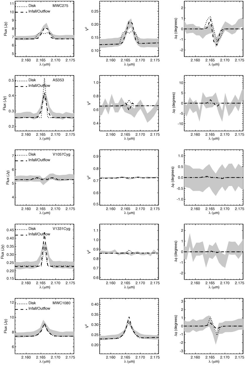
Figure 15: Figure 13 continued.

Figure 16: Inferred average stellocentric radius of Br$\gamma$ emission (from Table 3) plotted against the accretion luminosities derived for these objects (from Table 5).

Figure 17: Best-fit values of $R_{\rm in}$ for the infall/outflow models (from Table 4) plotted against the accretion luminosities derived for these objects (from Table 5). We only considered these two values of $R_{\rm in}$ in our modeling, which is why this plot is quantized.

References

- Acke et al. (2005) Acke, B., van den Ancker, M. E., & Dullemond, C. P. 2005, A&A, 436, 209
- Akeson et al. (2005a) Akeson, R. L., Boden, A. F., Monnier, J. D., Millan-Gabet, R., Beichman, C., Beletic, J., Calvet, N., Hartmann, L., Hillenbrand, L., Koresko, C., Sargent, A., & Tannirkulam, A. 2005a, ApJ, 635, 1173
- Akeson et al. (2005b) Akeson, R. L., Walker, C. H., Wood, K., Eisner, J. A., Scire, E., Penprase, B., Ciardi, D. R., van Belle, G. T., Whitney, B., & Bjorkman, J. E. 2005b, ApJ, 622, 440
- Benisty et al. (2010) Benisty, M., Natta, A., Isella, A., Berger, J., Massi, F., Le Bouquin, J., Mérand, A., Duvert, G., Kraus, S., Malbet, F., Olofsson, J., Robbe-Dubois, S., Testi, L., Vannier, M., & Weigelt, G. 2010, A&A, 511, 74
- Bertout et al. (1988) Bertout, C., Basri, G., & Bouvier, J. 1988, ApJ, 330, 350
- Bertout et al. (2007) Bertout, C., Siess, L., & Cabrit, S. 2007, A&A, 473, L21
- Boden et al. (1998) Boden, A. F., Colavita, M. M., van Belle, G. T., & Shao, M. 1998, in Proc. SPIE Vol. 3350, p. 872-880, Astronomical Interferometry, Robert D. Reasenberg; Ed., 872–880
- Calvet et al. (1991) Calvet, N., Hartmann, L., & Kenyon, S. J. 1991, ApJ, 383, 752
- Calvet et al. (2004) Calvet, N., Muzerolle, J., Briceño, C., Hernández, J., Hartmann, L., Saucedo, J. L., & Gordon, K. D. 2004, AJ, 128, 1294
- Carr (1989) Carr, J. S. 1989, ApJ, 345, 522
- Colavita et al. (2003) Colavita, M., Akeson, R., Wizinowich, P., Shao, M., Acton, S., Beletic, J., Bell, J., Berlin, J., Boden, A., Booth, A., Boutell, R., Chaffee, F., Chan, D., Chock, J., Cohen, R., Crawford, S., Creech-Eakman, M., Eychaner, G., Felizardo, C., Gathright, J., Hardy, G., Henderson, H., Herstein, J., Hess, M., Hovland, E., Hrynevych, M., Johnson, R., Kelley, J., Kendrick, R., Koresko, C., Kurpis, P., Le Mignant, D., Lewis, H., Ligon, E., Lupton, W., McBride, D., Mennesson, B., Millan-Gabet, R., Monnier, J., Moore, J., Nance, C., Neyman, C., Niessner, A., Palmer, D., Reder, L., Rudeen, A., Saloga, T., Sargent, A., Serabyn, E., Smythe, R., Stomski, P., Summers, K., Swain, M., Swanson, P., Thompson, R., Tsubota, K., Tumminello, A., van Belle, G., Vasisht, G., Vause, J., Walker, J., Wallace, K., & Wehmeier, U. 2003, ApJ, 592, L83
- Colavita (1999) Colavita, M. M. 1999, PASP, 111, 111
- Colavita & Wizinowich (2003) Colavita, M. M. & Wizinowich, P. L. 2003, in Interferometry for Optical Astronomy II. Edited by Wesley A. Traub. Proceedings of the SPIE, Volume 4838, pp. 79-88 (2003)., 79–88
- Dullemond et al. (2001) Dullemond, C. P., Dominik, C., & Natta, A. 2001, ApJ, 560, 957
- Edwards et al. (1994) Edwards, S., Hartigan, P., Ghandour, L., & Andrulis, C. 1994, AJ, 108, 1056
- Eisloeffel et al. (1990) Eisloeffel, J., Solf, J., & Boehm, K. H. 1990, A&A, 237, 369
- Eisner (2007) Eisner, J. A. 2007, Nature, 447, 562
- Eisner et al. (2007a) Eisner, J. A., Chiang, E. I., Lane, B. F., & Akeson, R. L. 2007a, ApJ, 657, 347
- Eisner et al. (2007b) Eisner, J. A., Graham, J. R., Akeson, R. L., Ligon, E. R., Colavita, M. M., Basri, G., Summers, K., Ragland, S., & Booth, A. 2007b, ApJ, 654, L77
- Eisner et al. (2009) Eisner, J. A., Graham, J. R., Akeson, R. L., & Najita, J. 2009, ApJ, 692, 309
- Eisner et al. (2005) Eisner, J. A., Hillenbrand, L. A., White, R. J., Akeson, R. L., & Sargent, A. I. 2005, ApJ, 623, 952
- Eisner et al. (2007c) Eisner, J. A., Hillenbrand, L. A., White, R. J., Bloom, J. S., Akeson, R. L., & Blake, C. H. 2007c, ApJ, 669, 1072
- Eisner et al. (2004) Eisner, J. A., Lane, B. F., Hillenbrand, L., Akeson, R., & Sargent, A. 2004, ApJ, 613, 1049
- Folha & Emerson (2001) Folha, D. F. M. & Emerson, J. P. 2001, A&A, 365, 90
- Hartmann (1998) Hartmann, L. 1998, Accretion processes in star formation (Accretion processes in star formation / Lee Hartmann. Cambridge, UK ; New York : Cambridge University Press, 1998. (Cambridge astrophysics series ; 32) ISBN 0521435072.)
- Hartmann et al. (2004) Hartmann, L., Hinkle, K., & Calvet, N. 2004, ApJ, 609, 906
- Hauschildt et al. (1999) Hauschildt, P. H., Allard, F., & Baron, E. 1999, ApJ, 512, 377
- Herbig & Jones (1983) Herbig, G. H. & Jones, B. F. 1983, AJ, 88, 1040
- Herbig et al. (2003) Herbig, G. H., Petrov, P. P., & Duemmler, R. 2003, ApJ, 595, 384
- Hessman & Guenther (1997) Hessman, F. V. & Guenther, E. W. 1997, A&A, 321, 497
- Hillenbrand et al. (1992) Hillenbrand, L. A., Strom, S. E., Vrba, F. J., & Keene, J. 1992, ApJ, 397, 613
- Isella & Natta (2005) Isella, A. & Natta, A. 2005, A&A, 438, 899
- Isella et al. (2008) Isella, A., Tatulli, E., Natta, A., & Testi, L. 2008, A&A, 483, L13
- Königl (1991) Königl, A. 1991, ApJ, 370, L39
- Konigl & Pudritz (2000) Konigl, A. & Pudritz, R. E. 2000, Protostars and Planets IV, 759
- Kraus et al. (2008) Kraus, S., Hofmann, K.-H., Benisty, M., Berger, J.-P., Chesneau, O., Isella, A., Malbet, F., Meilland, A., Nardetto, N., Natta, A., Preibisch, T., Schertl, D., Smith, M., Stee, P., Tatulli, E., Testi, L., & Weigelt, G. 2008, A&A, 489, 1157
- Kurosawa et al. (2006) Kurosawa, R., Harries, T. J., & Symington, N. H. 2006, MNRAS, 370, 580
- Lynden-Bell & Pringle (1974) Lynden-Bell, D. & Pringle, J. E. 1974, MNRAS, 168, 603
- Malbet et al. (2007) Malbet, F., Benisty, M., de Wit, W.-J., Kraus, S., Meilland, A., Millour, F., Tatulli, E., Berger, J.-P., Chesneau, O., Hofmann, K.-H., Isella, A., Natta, A., Petrov, R. G., Preibisch, T., Stee, P., Testi, L., Weigelt, G., Antonelli, P., Beckmann, U., Bresson, Y., Chelli, A., Dugué, M., Duvert, G., Gennari, S., Glück, L., Kern, P., Lagarde, S., Le Coarer, E., Lisi, F., Perraut, K., Puget, P., Rantakyrö, F., Robbe-Dubois, S., Roussel, A., Zins, G., Accardo, M., Acke, B., Agabi, K., Altariba, E., Arezki, B., Aristidi, E., Baffa, C., Behrend, J., Blöcker, T., Bonhomme, S., Busoni, S., Cassaing, F., Clausse, J.-M., Colin, J., Connot, C., Delboulbé, A., Domiciano de Souza, A., Driebe, T., Feautrier, P., Ferruzzi, D., Forveille, T., Fossat, E., Foy, R., Fraix-Burnet, D., Gallardo, A., Giani, E., Gil, C., Glentzlin, A., Heiden, M., Heininger, M., Hernandez Utrera, O., Kamm, D., Kiekebusch, M., Le Contel, D., Le Contel, J.-M., Lesourd, T., Lopez, B., Lopez, M., Magnard, Y., Marconi, A., Mars, G., Martinot-Lagarde, G., Mathias, P., Mège, P., Monin, J.-L., Mouillet, D., Mourard, D., Nussbaum, E., Ohnaka, K., Pacheco, J., Perrier, C., Rabbia, Y., Rebattu, S., Reynaud, F., Richichi, A., Robini, A., Sacchettini, M., Schertl, D., Schöller, M., Solscheid, W., Spang, A., Stefanini, P., Tallon, M., Tallon-Bosc, I., Tasso, D., Vakili, F., von der Lühe, O., Valtier, J.-C., Vannier, M., & Ventura, N. 2007, A&A, 464, 43
- Millan-Gabet et al. (2007) Millan-Gabet, R., Malbet, F., Akeson, R., Leinert, C., Monnier, J., & Waters, R. 2007, in Protostars and Planets V, ed. B. Reipurth, D. Jewitt, & K. Keil, 539–554
- Millan-Gabet et al. (2001) Millan-Gabet, R., Schloerb, F. P., & Traub, W. A. 2001, ApJ, 546, 358
- Monin et al. (1998) Monin, J.-L., Menard, F., & Duchene, G. 1998, A&A, 339, 113
- Monnier (2007) Monnier, J. D. 2007, New Astronomy Review, 51, 604
- Monnier et al. (2006) Monnier, J. D., Berger, J.-P., Millan-Gabet, R., Traub, W. A., Schloerb, F. P., Pedretti, E., Benisty, M., Carleton, N. P., Haguenauer, P., Kern, P., Labeye, P., Lacasse, M. G., Malbet, F., Perraut, K., Pearlman, M., & Zhao, M. 2006, ApJ, 647, 444
- Monnier et al. (2005) Monnier, J. D., Millan-Gabet, R., Billmeier, R., Akeson, R. L., Wallace, D., Berger, J.-P., Calvet, N., D’Alessio, P., Danchi, W. C., Hartmann, L., Hillenbrand, L. A., Kuchner, M., Rajagopal, J., Traub, W. A., Tuthill, P. G., Boden, A., Booth, A., Colavita, M., Gathright, J., Hrynevych, M., Le Mignant, D., Ligon, R., Neyman, C., Swain, M., Thompson, R., Vasisht, G., Wizinowich, P., Beichman, C., Beletic, J., Creech-Eakman, M., Koresko, C., Sargent, A., Shao, M., & van Belle, G. 2005, ApJ, 624, 832
- Muzerolle et al. (2001) Muzerolle, J., Calvet, N., & Hartmann, L. 2001, ApJ, 550, 944
- Muzerolle et al. (2003) Muzerolle, J., Calvet, N., Hartmann, L., & D’Alessio , P. 2003, ApJ, 597, L865
- Muzerolle et al. (1998) Muzerolle, J., Hartmann, L., & Calvet, N. 1998, AJ, 116, 2965
- Najita et al. (1996) Najita, J., Carr, J. S., & Tokunaga, A. T. 1996, ApJ, 456, 292
- Najita et al. (2007) Najita, J. R., Carr, J. S., Glassgold, A. E., & Valenti, J. A. 2007, in Protostars and Planets V, B. Reipurth, D. Jewitt, and K. Keil (eds.), University of Arizona Press, Tucson, 951 pp., 2007., p.507-522, ed. B. Reipurth, D. Jewitt, & K. Keil, 507–522
- Perryman et al. (1997) Perryman, M. A. C., Lindegren, L., Kovalevsky, J., Hoeg, E., Bastian, U., Bernacca, P. L., Crézé, M., Donati, F., Grenon, M., van Leeuwen, F., van der Marel, H., Mignard, F., Murray, C. A., Le Poole, R. S., Schrijver, H., Turon, C., Arenou, F., Froeschlé, M., & Petersen, C. S. 1997, A&A, 323, L49
- Pott et al. (2010) Pott, J.-U., et al. 2010, ApJ, submitted
- Prato et al. (2003) Prato, L., Greene, T. P., & Simon, M. 2003, ApJ, 584, 853
- Shu et al. (1994) Shu, F., Najita, J., Ostriker, E., Wilkin, F., Ruden, S., & Lizano, S. 1994, ApJ, 429, 781
- Steenman & Thé (1991) Steenman, H. & Thé, P. S. 1991, Ap&SS, 184, 9
- Tannirkulam et al. (2008) Tannirkulam, A., Monnier, J. D., Millan-Gabet, R., Harries, T. J., Pedretti, E., ten Brummelaar, T. A., McAlister, H., Turner, N., Sturmann, J., & Sturmann, L. 2008, ApJ, 677, L51
- Tatulli et al. (2007) Tatulli, E., Isella, A., Natta, A., Testi, L., Marconi, A., Malbet, F., Stee, P., Petrov, R. G., Millour, F., Chelli, A., Duvert, G., Antonelli, P., Beckmann, U., Bresson, Y., Dugué, M., Gennari, S., Glück, L., Kern, P., Lagarde, S., Le Coarer, E., Lisi, F., Perraut, K., Puget, P., Rantakyrö, F., Robbe-Dubois, S., Roussel, A., Weigelt, G., Zins, G., Accardo, M., Acke, B., Agabi, K., Altariba, E., Arezki, B., Aristidi, E., Baffa, C., Behrend, J., Blöcker, T., Bonhomme, S., Busoni, S., Cassaing, F., Clausse, J.-M., Colin, J., Connot, C., Delboulbé, A., Domiciano de Souza, A., Driebe, T., Feautrier, P., Ferruzzi, D., Forveille, T., Fossat, E., Foy, R., Fraix-Burnet, D., Gallardo, A., Giani, E., Gil, C., Glentzlin, A., Heiden, M., Heininger, M., Hernandez Utrera, O., Hofmann, K.-H., Kamm, D., Kiekebusch, M., Kraus, S., Le Contel, D., Le Contel, J.-M., Lesourd, T., Lopez, B., Lopez, M., Magnard, Y., Mars, G., Martinot-Lagarde, G., Mathias, P., Mège, P., Monin, J.-L., Mouillet, D., Mourard, D., Nussbaum, E., Ohnaka, K., Pacheco, J., Perrier, C., Rabbia, Y., Rebattu, S., Reynaud, F., Richichi, A., Robini, A., Sacchettini, M., Schertl, D., Schöller, M., Solscheid, W., Spang, A., Stefanini, P., Tallon, M., Tallon-Bosc, I., Tasso, D., Vakili, F., von der Lühe, O., Valtier, J.-C., Vannier, M., & Ventura, N. 2007, A&A, 464, 55
- Tatulli et al. (2008) Tatulli, E., Malbet, F., Ménard, F., Gil, C., Testi, L., Natta, A., Kraus, S., Stee, P., & Robbe-Dubois, S. 2008, A&A, 489, 1151
- White & Ghez (2001) White, R. J. & Ghez, A. M. 2001, ApJ, 556, 265
- Woillez et al. (2010) Woillez, J., et al. 2010, PASP, submitted