Electron Phenomena in Layered Conductors

O.V. KIRICHENKO, Yu.A. KOLESNICHENKO

and V.G. PESCHANSKY

B.I. Verkin Institute for Low Temperature Physics and Engineering,

National Academy of Sciences of the Ukraine

ABSTRACT

The quasi-two-dimensional nature of the charge carriers energy spectrum in layered conductors leads to specific effects in an external magnetic field. The magnetoresistance of layered conductors in a wide range of strong magnetic fields directed in the plane of the layers can increase proportionally to a magnetic field value. The electromagnetic impedance and the sound attenuation rate depend essentially on the polarization of normal to the layers. Propagation of electromagnetic and acoustic waves in these conductors involves virtually all charge carriers in the transfer of acoustic pulses and electromagnetic field spikes to the bulk of the conductor. The orbits of Fermi electrons in a magnetic field are virtually indistinguishable, which allows the inclusion of large number of conduction electrons in the formation of peculiar oscillatory and resonant effects which are absent in the case of ordinary metals. Investigation of these effects introduce the possibilities for detailed study of the dissipative processes in electron systems of layered conductors and the charge carriers energy spectrum.

Point contact investigations of layered metals allow us to obtain the information about electron and phonon spectra. The electron focusing signal and the point contact spectrum are extremely sensitive to the orientation of the magnetic field vector $\boldsymbol{H}$ in relation to the layers with a high electrical conductivity. The values of $\boldsymbol{H}$ for which the electron focusing signal has peaks can be used for determining velocities and extremal diameters for the open Fermi surface. The dependence of the point contact spectra on the magnitude and the relaxation of electrons at various types of phonon excitations.

Electron Phenomena in Layered Conductors

CONTENTS

1. INTRODUCTION

The search for new superconducting materials has focused attention on conductors of organic origin, which possess layered of thread structure with a pronounced anisotropy in the normal (non-superconducting) state. Many of them have the metal-type electrical conductivity, i.e. their resistance increases with increasing temperature and are known as artificial or synthetic metals. However, the electron properties of low-dimensional conductors differ essentially from those of ordinary metals, and the utilization of layered and thread conductors in different spheres of the modern electronics appears to be more effective than metals and semiconductors. In this connection it is useful to make a theoretical analysis of the electron processes proceeding in low-dimensional conductors.

It is of interest to investigate to what extent layered conductors are also the preferred objects for the investigations of the Kapitza’s effect.

A considerable part of organic superconductors are layered structures, and their conductivity along the layers is significantly higher than along the normal $\boldsymbol{n}$ to the layers. Many layered conductors, in particular halides of tetraseleniumtetracen and salts of tetrahiafulvalene, exhibit the metal type conductivity even across the layers. Thus there are grounds for making use of the concept of quasiparticles carrying a charge $e$, analogous to conduction electrons in metals, in order to describe electron processes in such conductors. Evidently, sharp anisotropy of the electrical conductivity is connected with the anisotropy of the charge carriers velocity $\boldsymbol{v}=\partial\varepsilon(\boldsymbol{p})/\partial p$ on the Fermi surface $\varepsilon(\boldsymbol{p})=\varepsilon_{\rm F}$, i.e. their energy

$$\varepsilon(\boldsymbol{p})=\sum_{n=0}^{\infty}\varepsilon_{n}(p_{x},p_{y})\cos\left\{\frac{anp_{z}}{\hbar}\right\}$$ (1.1)

is weakly dependent on the quasi-momentum projection $p_{z}=\boldsymbol{pn}$. The Fermi surface of such conductors represents a weakly corrugated cylinder and, probably, some more closed cavities referring to the small groups of charge carriers.

Here $a$ is the separation between the layers, $\hbar$ is the Planck constant, the maximum values on the Fermi surface of the function $\varepsilon_{1}(p_{x},p_{y})$ is $\eta\varepsilon_{\rm F}\ll\varepsilon_{\rm F}$, and of the functions $\varepsilon_{n}(p_{x},p_{y})$ with $n\geq 2$ being equal to $A_{n}$, is still smaller, i.e. $A_{n+1}\ll A_{n}$. Such form is characteristic of the charge carriers dispersion low in the strong coupling approximation when the overlap of the wave functions of electrons belonging to different bands is negligible.

Below we consider electron phenomena in layered conductors with the metal-type conductivity for the most general assumptions on the form of the quasi-two-dimensional electron energy spectrum.

2. GALVANOMAGNETIC EFFECTS

In contrast to the case of a metal, in the layered conductors placed in a magnetic field $\boldsymbol{H}$ both the absence of a response to the action of the field and the intensification of galvanomagnetic effects, characteristic of metals, are possible.

In 1928, P.L. Kapitza observed a wonderful phenomena – the linear growth with a magnetic field of the resistance of metals at liquid air and liquid carbon oxide temperature ranges [1]. For this purpose Kapitza created powerful magnets, in which the magnetic field attains 30–50 tesla. At that time in Leiden experimental investigations at lower temperatures were carried out, which raised the effectiveness of less strong magnetic fields by increasing the charge carriers mean free path. At liquid hydrogen temperatures instead of the linear increase of the magnetic field, the more complicated dependence of the resistance of single bismuth crystals was observed by Shubnikov and de Haas [2], and at helium temperatures the oscillatory dependence of the resistance on the inverse magnetic field – the Shubnikov–de Haas effect – was clearly demonstrated [3]. The oscillatory dependence is a common effect for metals, which is connected with the presence of the singularities of the density of states of the charge carriers while their energy spectrum is quantized by a magnetic field [4]. The amplitude of the quantum oscillations in metals is substantially less than the amplitude of the oscillations observed in bismuth, which is caused, by the sharp anisotropy of the Fermi surface of bismuth-type semimetals.

The Shubnikov–de Haas effect is also clearly manifested in the tetrathiafulvalene salts and halides of tetraseleniumtetracen, which have a pronounced layered structure [5–14]. A considerable increase in the amplitude of the quantum oscillations of the magnetoresistance in the layered conductors arises from the quasi-two-dimensial character of their electron energy spectrum. In metals, the Shubnikov–de Haas effect is formed only by the small fractions of charge carriers on the Fermi surface. These are electrons near the Fermi surface cross-sections whose areas cut by the plane $p_{\rm H}=\boldsymbol{pH}/H=\mbox{const}$ are close to the extreme magnitude [15–16], or conduction electrons near the self-intersecting orbit [17]. In contrast to metals, in the quasi-two-dimensional conductors almost all charge carriers with the Fermi energy contribute to the quantum oscillatory effects because at $\eta\ll 1$ all closed cross-sections of the Fermi surface cut by the plane $p_{\rm H}=\mbox{const}$ are almost indistinguishable.

It is also of interest to find out to what extent the layered conductors are preferable objects for the investigations of the Kapitza’s effect as well.

The linear growth of the resistance observed by Kapitza was not in agreement with the main principles of the electron theory of metals, because in accordance with the Onsager principle of symmetry of kinetic coefficients [18] the resistance of a conductor must be an even function of a magnetic field. The first attempt to explain the results of the Kapitza’s experiments was made only 30 years later. The agreement with the Onsager principle of the linear increase with $\boldsymbol{H}$ of the resistance is related to the complicated form of the dependence of the charge carriers energy $\varepsilon$ upon their quasimomentum $\boldsymbol{p}$. The fundamental characteristic of the electron energy spectrum – the Fermi surface – is open for almost all metals, and in a magnetic field the orbits of electrons with the Fermi energy $\varepsilon_{\rm F}$ can pass through a large number of cells in the momentum space. The period of revolution of conduction electrons on such strongly elongated orbits $T=2\pi/\Omega$ may be greater than its free path time $\tau$ at however strong magnetic field. As a result averaging of the resistance of a polycrystal wire over all possible orientations of crystallites and, consequently, over electron orbits leads to the linear dependence of the resistance on the magnitude of a strong magnetic field ($\Omega_{0}\tau\gg 1$, where $\Omega_{0}$ is the maximum rotational frequency of the Fermi electron in a magnetic field) [19, 20]. If the thickness of a polycrystal specimen of a metal f with an open Fermi surface significantly exceeds the crystallite dimension, then in a strong magnetic field the resistance $\rho$ is proportional to $H^{4/3}$ [21, 22], i.e. the $H$-dependence of $\rho$ is close to the linear one. If there are saddle points on the Fermi surface the frequency of revolution takes on all values within the interval between zero and $\Omega_{0}$ in a single crystal. This is the case when self-intersecting orbits, on which an electron cannot make a total revolution, may take place. However, a number of electrons near the self-intersecting orbit, for which the period $T$ is greater than the free path time, is proportional to $\exp(-\Omega_{0}\tau)$, because the period as a function of $p_{\rm H}=\boldsymbol{pH}/H$ diverges logarithmically on the self-intersecting orbit. As a result, in a very narrow range of magnetic fields the complicated dependence of $\rho$ upon $H$ changes for the saturation or the quadratical growth with increasing $H$.

In the quasi-two-dimensional conductors the period of revolution of charge carriers in a magnetic field is weakly dependent on the momentum projection $p_{\rm H}$, and there are grounds to expect that in such conductors a number of electrons near the self-intersecting orbit, for which $T>\tau$, is essentially greater than in an ordinary metal. These electrons, make a major contribution to conductivity in a significantly wider range of magnetic fields ($\Omega\tau\gg 1$), and averaging of the frequencies of revolution will give another result in comparison with the case of a metal. In order to find out the connection between the current density

$$j_{i}=\frac{2}{(2\pi\hbar)^{3}}\int ev_{i}f(\boldsymbol{p})\,\mbox{d}^{3}p=\sigma_{ik}E_{k}$$ (2.1)

and electric field $\boldsymbol{E}$ it is necessary to solve the kinetic equation for the charge carriers distribution function $f(\boldsymbol{p})$

$$\left(e\boldsymbol{E}+\frac{[\boldsymbol{v}\boldsymbol{H}e]}{c}\right)\frac{\partial f}{\partial p}=W_{\rm col}\{f\}.$$ (2.2)

At small electric field the deviation of the distribution function

$$f(\boldsymbol{p})=f_{0}(\varepsilon)-eE_{i}\psi_{i}(\boldsymbol{p})\frac{\partial f_{0}(\varepsilon)}{\partial\varepsilon}$$ (2.3)

from the equilibrium Fermi function $f_{0}(\varepsilon)$ is small and the kinetic equation (2.2) can be linearized in small perturbation of the conduction electrons system. In this approximation the collision integral $W_{\rm col}$ represents a linear integral operator applying to $\psi_{i}$, which is the function to be found. At low temperatures when conduction electrons are scattered mainly by impurities and crystal defects, we may take, with sufficient accuracy, the collision integral to be the operator of multiplication by the collision frequency $1/\tau$ of the unequilibrium correction to the Fermi function $f_{0}(\varepsilon)$, i.e. the solution of the kinetic equation appears to be the proper function of the integral operator of collisions. When taking into account the other mechanisms of dissipation, the solution of the kinetic equation should be found in the basis of proper functions of the collision integral operator, but a correct solution of this complicated mathematical problem only enables us to improve unessential numerical factors of the order of unity and does not touch the functional behaviour of the physical characteristics of a conductor, i.e. their dependence on external parameters. In order to find out the dependence of the resistance and the Hall field in the layered conductor on the magnitude and orientation of a magnetic field, the $\tau$-approximation for the collision integral is used. In this approximation the kinetic equation takes the simple enough form

$$\frac{e}{c}[\boldsymbol{v}\times\boldsymbol{H}]\frac{\partial\psi_{i}}{\partial\boldsymbol{p}}+\frac{\psi_{i}}{\tau}=v_{i},$$ (2.4)

and its solution

$$\psi_{i}(t,p_{\rm H},\varepsilon)=\int^{t}_{-\infty}v_{i}(t^{\prime},p_{\rm H},\varepsilon)\exp\left\{\frac{t^{\prime}-t}{\tau}\right\}\,\mbox{d}t^{\prime}$$ (2.5)

allows us to determine the components of the electrical conductivity tensor

$$\sigma_{ik} = -\frac{2e^{3}H}{c(2\pi\hbar)^{3}}\int\mbox{d}\varepsilon\,\frac{\partial f_{0}}{\partial\varepsilon}\,\int\mbox{d}p_{\rm H}\,\int_{0}^{T}\mbox{d}t\,v_{i}(t)$$ (2.6)

$$\times \int^{t}_{-\infty}v_{k}(t^{\prime})\exp\left\{\frac{t^{\prime}-t}{\tau}\right\}\,\mbox{d}t^{\prime}$$

$$= \langle e^{2}v_{i}\psi_{k}\rangle.$$

As the variables in the momentum space we have chosen the integrals of motion $\varepsilon$, $p_{\rm H}$ and the time $t$ of electron motion in a magnetic field $\boldsymbol{H}=(0,H\sin\theta,H\cos\theta)$ according to the equations

$$\frac{\partial p_{x}}{\partial t} = \frac{eH}{c}(v_{y}\cos\theta-v_{z}\sin\theta);$$

$$\frac{\partial p_{y}}{\partial t} = -\frac{eH}{c}v_{x}\cos\theta;$$

$$\frac{\partial p_{y}}{\partial t} = \frac{eH}{c}v_{x}\sin\theta.$$ (2.7)

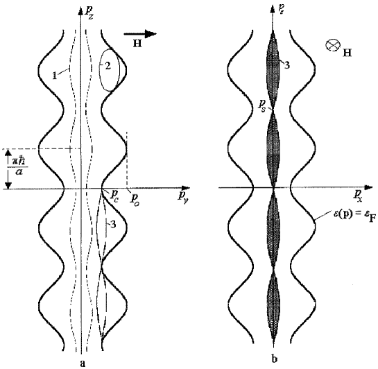
Figure 1: Different types of electron trajectories in the momentum space in a magnetic field applied parallel to the layers: 1, an open trajectory; 2, a closed orbit; 3, the self-intersecting orbit containing the saddle points $\boldsymbol{p}_{\rm s}$. The cross-section $p_{y}=p_{\rm c}$ separates the region of open cross-sections from the closed ones.

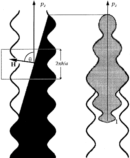
Figure 2: Electron trajectories on the Fermi surface in an oblique magnetic field ($\theta$ is the angle of deviation of the vector $\boldsymbol{H}$ from the layers-plane). An electron orbit (1) passes through a few number of cells in the momentum space.

Suppose the Fermi surface of the layered conductor with the quasi-two-dimensional energy spectrum to be only one weakly corrugated cylinder with the direction of “openness” aligned with the $p_{z}$-axis (Fig. 1). If $\theta$ differs from $\pi/2$, all cross-sections of the weakly corrugated cylinder cut by the plane $\boldsymbol{pH}=\mbox{const}$ are closed and almost indistinguishable for $\eta\ll 1$ (Fig. 2). The angle $\theta$ approaching $\pi/2$, closed electron orbit becomes strongly elongated, and at $\theta=\pi/2$ transforms into two open orbits (Fig. 1). The period of motion changes discontinually and on the open cross-section cut by the plane $p_{\rm H}=p_{y}=\mbox{const}$, takes the form

$$T=\frac{2\pi m^{*}c}{eH}=\frac{c}{eH}\int\limits_{0}^{2\pi\hbar/a}\frac{\mbox{d}p_{z}}{v_{x}}.$$ (2.8)

When approaching the limiting cross-section $p_{y}=p_{\rm c}$, which separates the region of open cross-sections from the small layer of closed ones, the period of motion $T(p_{y})$ increases without limit. This results from the fact that the cross-section $p_{y}=p_{\rm c}$ contains the saddle points $\boldsymbol{p}_{\rm c}=(0,p_{\rm c},2\pi\hbar n/a)$, where open orbits touch one another, and electrons make a long stay near the points of self-intersection because their velocity in the plane orthogonal to $\boldsymbol{H}$ is negligible (Fig. lb).

At $\theta=\pi/2$ the mean value of the velocity $v_{x}$ differs from zero

$${\bar{v}}_{x}=T^{-1}\int\limits_{0}^{T}\mbox{d}t\,v_{x}(t)=\frac{2\pi\hbar ec}{aHT}=\frac{h}{am^{*}},$$ (2.9)

and all directions of drift the charge carriers cover the whole $xy$-plane. In this case the components of the electrical conductivity tensor $\sigma_{xx}$ and $\sigma_{yy}$ coincide in order of magnitude with the conductivity along the layers in the absence of a magnetic field. However, at $\eta\ll 1$ the components of the tensor $\sigma_{ij}$ with one or two $z$ indices are incredible small and in a strong magnetic field they also decrease with increasing $H$ because ${\bar{v}}_{z}=0$.

Being determined up to terms proportional to $\eta$, the period of motion along an orbit sufficiently distant from the self-intersecting one, is inversely proportional to $v_{x}(0)$ (we have taken the central cross-section $p_{z}=0$ as the origin of the variable $t$). When an electron approaches the self-intersecting orbit $p_{y}=p_{\rm c}$, its velocity along the $x$-axis decreases and allowance for small corrections in $\eta$ becomes necessary. The period of motion of electrons along the orbit on which $p_{\rm H}$ is close to $p_{\rm c}$ is very large, since electrons stay for a long time near the saddle point $\boldsymbol{p}_{\rm c}=(0,p_{\rm c},0)$, where $v_{x}=v_{z}=0$ (see Fig. lb). In the vicinity of the cross-section $p_{\rm H}=p_{\rm c}$ the electron velocity projection $v_{x}$ is a complicated function of $t$, but far from this cross-section the small corrections in $\eta$ depending on $t$ can be omitted in the expression for $v_{x}(t)$. The period of charge carriers motion has the form

$$T(p_{\rm H})=\frac{2\pi\hbar c}{aeHv_{y}(0)}=\frac{2\pi v_{\rm F}}{\Omega_{0}v_{x}(0)}$$ (2.10)

and at $v_{x}\ll v_{\rm F}=\varepsilon_{\rm F}a/\hbar$ may become comparable with the free path time. As a result the charge carriers with the small value of the velocity projection $v_{x}$ give the major contribution into $\sigma_{iz}$ and $\sigma_{zi}$. Regardless of the small corrections depending on $t$, $p_{z}$ is the linear function of the time of motion in a magnetic field, and the velocity projection

$$v_{z}=-\sum\limits_{n=1}^{\infty}\frac{an}{\hbar}\varepsilon_{n}(p_{x},p_{y})\sin(n\Omega t)$$ (2.11)

is determined mainly by the first term in Equation (2.11). It is not difficult to calculate the conductivity component $\sigma_{zz}$ in this case:

$$\sigma_{zz}=\frac{2e^{2}\tau}{(2\pi\hbar)^{3})}\int 2\pi m^{*}\,\mbox{d}p_{\rm H}\,\sum\limits_{n=1}^{\infty}\frac{\{\varepsilon_{n}(p_{x},p_{y})an/\hbar^{2}\}}{1+(n\Omega\tau)^{2}}.$$ (2.12)

In the vicinity of the cross-section $p_{\rm H}=p_{\rm c}$ the numerators in Equation (2.12) should be improved by changing them for $|v_{z}^{n}|^{2}$. Since for these charge carriers $p_{z}$ is a complicated function of $t$, the Fourier transforms of the velocities $v_{z}^{n}$ need not be decreasing with $n$, and the contribution in the asymptotic value of $\sigma_{zz}$ from electrons belonging to the vicinity of the saddle point is not limited only by the first harmonic in the Fourier expansion of the function $v_{z}(t)$. At the limiting cross-section $p_{y}=p_{\rm c}$ the maximum value of the velocity of electron motion along the $x$-axis is equal in the order of magnitude to $\eta^{1/2}v_{\rm F}$ and $t$-dependence of $v_{x}$ is of no importance only at $v_{x}(0)\gg\eta^{1/2}v_{\rm F}$.

Let $\sigma_{zz}$ be represented in the form $\sigma_{zz}=\sigma_{zz}^{(1)}+\sigma_{zz}^{(2)}+\sigma_{zz}^{(3)}$, where $\sigma_{zz}^{(1)}$ describes the contribution of the charge carriers whose velocity $v_{z}$ is given by Equation (2.11), the second term is the contribution to $\sigma_{zz}$ from conduction electrons on the open orbits for which $v_{x}\leq\eta^{1/2}v_{\rm F}$, and the last term

$$\sigma_{zz}^{(3)}=\frac{4e^{2}\tau}{(2\pi\hbar)^{3}}\int\limits_{p_{\rm c}}^{p_{0}}\mbox{d}p_{\rm H}\,2\pi m^{*}(p_{\rm H})\sum\limits_{m=1}^{\infty}\frac{|v_{z}^{n}|^{2}}{1+(n\Omega\tau)^{2}}$$ (2.13)

is connected with the charge carriers on the closed orbits.

Here $p_{0}$ is the maximum value of $p_{\rm H}$ in the Fermi surface reference point $\boldsymbol{p}_{0}=(0,p_{0},\pi h/a)$ (Fig. la).

At $\gamma_{0}=1/\Omega_{0}\tau>\eta^{1/2}$ the integration in $p_{\rm H}$ over a small interval where $\eta^{1/2}v_{\rm F}<v_{x}\ll v_{\rm F}$ leads to the following result

$$\sigma_{zz}^{(1)}=\sigma_{0}\eta^{2}\gamma_{0},$$ (2.14)

where $\sigma_{0}$ is of the order of the conductivity along the layers in the absence of a magnetic field.

Near the reference point of the Fermi surface the charge carriers cyclotron mass $m^{*}$ is proportional to $\eta^{-1/2}$ and increases when approaching to the cross-section $p_{\rm H}=p_{\rm c}$, on which it becomes infinite. At $\eta^{1/2}\ll\gamma_{0}$ conduction electrons on the closed cross-sections have no time to make a total revolution along the orbit and give the following contribution into $\sigma_{zz}$:

$$\sigma_{zz}^{(3)}=\frac{4e^{2}\tau}{(2\pi\hbar)^{3}}\int\limits_{p_{\rm c}}^{p_{0}}2\pi m^{*}(p_{\rm H})\,\mbox{d}p_{\rm H}\,{\bar{v}}_{z}^{2}=\sigma_{0}\eta^{5/2}.$$ (2.15)

Here and below we shall omit unessential factors of the order of unity in formulas for $\sigma_{zz}$.

Thus, at $\eta^{1/2}\ll\gamma_{0}\ll 1$ a small fraction of conduction electrons on the open orbits moving slowly along the $x$-axis gives the main contribution to $\sigma_{zz}$.

A number of conduction electrons for which $T>\tau$ decreases with increasing magnetic field, and the contribution to $\sigma_{zz}$ of the charge carriers on the orbits close to the cross-section $p_{\rm H}=p_{\rm c}$ becomes essential. Near the self-intersecting orbit the charge carriers velocity projection $v_{x}$ is small, i.e. their energy is weakly dependent on $p_{x}$, and we can easily find the $p_{\rm H}$-dependence of the period of motion from the expansion of the energy in the powers of $p_{x}$. We retain only the first two terms in Equation (1.1), viz.

$$\varepsilon(\boldsymbol{p})=\varepsilon(0,p_{y})+\frac{p_{x}^{2}}{2m_{1}}+\varepsilon_{1}(0,p_{y})\cos\left(\frac{ap_{z}}{\hbar}\right).$$ (2.16)

Using Equation (2.7) we obtain

$$T(p_{\rm H})=\frac{\hbar c}{aeH}\left\{\frac{m_{1}}{\varepsilon_{1}(0,p_{y})}\right\}^{1/2}\int\limits_{0}^{\pi}\mbox{d}\alpha\,(\xi^{2}+\sin^{2}\alpha)^{1/2},$$ (2.17)

where

$$\xi^{2}=\frac{\varepsilon_{0}(0,p_{\rm c})-\varepsilon(0,p_{y})+\varepsilon_{1}(0,p_{\rm c})-\varepsilon_{1}(0,p_{y})}{2\varepsilon_{1}(0,p_{y})}.$$

At $\xi\ll 1$ the period of motion of charge carriers

$$T(p_{\rm H})\cong\Omega_{0}^{-1}\eta^{-1/2}\ln\left(\frac{1}{\xi}\right)$$ (2.18)

diverges logarithmically, and the contribution into $\sigma_{zz}$ of electrons belonging to the small vicinity (of the order of $\Delta p_{\rm H}=p_{\rm c}-p_{\rm H}\cong p_{\rm c}\eta$) of the limiting cross-section has the form

$$\sigma_{zz}^{(2)}=\sigma_{0}\eta^{5/2}\gamma_{0}^{2}\int\limits_{\infty}^{1}\mbox{d}u\,\frac{u^{3}\exp\{-u\}}{u^{2}\gamma_{0}^{2}+\eta}\cong\sigma_{0}\frac{\gamma_{0}^{2}\eta^{5/2}}{\gamma_{0}^{2}+\eta}.$$ (2.19)

In ordinary metals the period of motion of charge carriers is greater or comparable with the free path time only in a small region (about $\exp[-\Omega_{0}\tau]$) of the Fermi surface self-intersecting cross-section. In contrast to the case of a metal, in the quasi-two-dimensional conductors the condition $T\geq\tau$ is satisfied in a wider range of electron orbits, where $\xi$ can be of the order of unity.

At $\eta^{1/2}\ll\gamma_{0}$ the contribution into $\sigma_{zz}$ of charge carriers in the vicinity of the self-intersecting cross-section of the order of $p_{0}\eta$ is very incredibly small and $\sigma_{zz}\cong\sigma_{zz}^{(1)}$, whereas in the opposite case these charge carriers contribute to conductivity on a level with other conduction electrons. It is easy to determine that at $\eta>\gamma_{0}^{2}$ the conductivity $\sigma_{zz}^{(1)}$ also decreases proportionally to $\gamma_{0}^{2}$ as a magnetic field increases. As a result, in the range of strong magnetic fields when $\gamma_{0}\leq\eta^{1/2}$, we have

$$\sigma_{zz}\cong\sigma_{0}\eta^{3/2}\gamma_{0}^{2}.$$ (2.20)

In the layered conductors the Hall field also behave differently to metals. In order to demonstrate the results obtained more visibly, we consider the galvanomagnetic phenomena using the simple model of the charge carriers dispersion law

$$\varepsilon(\boldsymbol{p})=\frac{p_{x}^{2}+p_{y}^{2}}{2m}-\eta\frac{v_{\rm F}\hbar}{a}\cos\left(\frac{ap_{z}}{\hbar}\right).$$ (2.21)

This is the approximation at which charge carriers are assumed to be almost free in the layers-plane. Since the main contribution to the electrical conductivity across the layers is given by electrons with small $v_{x}$-velocity and the dependence of $\varepsilon_{n}(p_{x},p_{y})$ on $p_{y}$ is nonessential at $\theta=\pi/2$, the analysis of the galvanomagnetic effects given below applies.

Making use of the equation of charge carriers motion in a magnetic field (2.7) at $\theta=\pi/2$ and of the dispersion law (2.21), we have

$$\psi_{z}=\gamma(\psi_{x}-v_{x}\tau),$$ (2.22)

where $\gamma=mc/eH\tau$. From this it follows that

$$\sigma_{zz}=\gamma\sigma_{zx};\quad\sigma_{xz}=\gamma(\sigma_{xx}-\sigma_{0});\quad\sigma_{zx}=-\sigma_{xz},$$ (2.23)

and the matrix $\sigma_{ij}$ has the form

$$\sigma_{ij}=\left(\begin{array}[]{ccc}\sigma_{0}-\gamma^{-2}\sigma_{zz}&0&-\gamma^{-1}\sigma_{zz}\\ 0&\sigma_{0}&0\\ \gamma^{-1}\sigma_{zz}&0&\sigma_{zz}\end{array}\right).$$ (2.24)

For the inverse tensor of the resistance we have

$$\rho_{ij}=\left(\begin{array}[]{ccc}\sigma_{0}^{-1}&0&-(\gamma\sigma_{0})^{-1}\\ 0&\sigma_{0}^{-1}&0\\ (\gamma\sigma_{0})^{-1}&0&\sigma_{zz}^{-1}-\sigma_{0}^{-1}\gamma^{-2}\end{array}\right).\vspace{6pt}$$ (2.25)

It can be seen that the resistance along the normal to the layers $\rho_{zz}$ to a good accuracy is equal to $1/\sigma_{zz}$ and grows linearly with a magnetic field at $\eta^{1/2}\ll\gamma\ll 1$. The Hall field

$$\boldsymbol{E}_{\rm Hall}=R[\boldsymbol{j}\times\boldsymbol{H}]\vspace{5pt}$$ (2.26)

is also proportional to $H$, and the Hall constant $R$ is inversely proportional to the volume within the Fermi surface. In metals, the Hall constant is of the same form only in the absence of the Fermi surface open cross-sections.

The absence of the magnetoresistance $\Delta\rho=\rho(H)-\rho(0)$ for the current directed along the layers is connected with the quadratical dispersion of the charge carriers in the $xy$-plane. For more complicated dependence of the charge carriers energy on $p_{x}$ and $p_{y}$ the resistance grows with increasing $H$ and tends to a finite value in a high magnetic field, as demonstrated in metals. However, the opposite occur in case of a metal, and the quasi-two-dimensional conductors $\Delta\rho$ is very small and disappears at $\eta=0$. This follows from the fact that the only projection onto the normal to the layers of a magnetic field, which disappears at $\theta=\pi/2$, fundamentally affects the charge carriers dynamics.

For $(\pi/2)\leq\eta$ the conductivity along the layers is similar to that in the absence of a magnetic field, and the Equations (2.14) and (2.20) are valid for $\sigma_{zz}$ until $\gamma_{0}\geq\eta$. But at $(\pi/2-\theta)\gg\eta$ there are no self-intersecting orbits, and in actually attained strong magnetic fields the in-plane resistance tends to a finite value in a large range of angles $\theta$ of deviation of the field from the layers-plane.

Using Equation (2.21) for the cargo carriers dispersion law, we have for the conductivity tensor

$$\sigma_{ij}=\left(\begin{array}[]{ccc}\displaystyle\frac{\sigma_{xy}\gamma_{0}}{\cos\theta}&\sigma_{xy}&\displaystyle-\frac{\sigma_{zz}\gamma_{0}\sin\theta}{\gamma_{0}^{2}+\cos^{2}\theta}\\[8.0pt] -\sigma_{xy}&\displaystyle\sigma_{0}-\frac{\sigma_{xy}\cos\theta}{\gamma_{0}}&\displaystyle\frac{\sigma_{zz}\sin\theta\cos\theta}{\gamma_{0}^{2}+\cos^{2}\theta}\\[8.0pt] \displaystyle\frac{\sigma_{zz}\gamma_{0}\sin\theta}{\gamma_{0}^{2}+\cos^{2}\theta}&\displaystyle\frac{\sigma_{zz}\sin\theta\cos\theta}{\gamma_{0}^{2}+\cos^{2}\theta}&\sigma_{zz}\end{array}\right);$$ (2.27)

and for the resistance tensor

$$\rho_{ij}=\left(\begin{array}[]{ccc}\sigma_{0}^{-1}&\displaystyle\frac{H\cos\theta}{Nec}&\displaystyle-\frac{H\sin\theta}{Nec}\\[8.0pt] \displaystyle-\frac{H\cos\theta}{Nec}&\sigma_{0}^{-1}&0\\[8.0pt] \displaystyle\frac{H\sin\theta}{Nec}&0&\displaystyle\sigma_{zz}^{-1}-\frac{\sin^{2}\theta}{\sigma_{0}(\gamma^{2}+\cos^{2}\theta)}\end{array}\right);$$ (2.28)

where

$$\sigma_{xy}=\frac{\gamma_{0}\cos\theta}{(\gamma_{0}^{2}+\cos^{2}\theta)^{2}}[\sigma_{0}(\gamma_{0}^{2}+\cos^{2}\theta)-\sigma_{zz}\sin\theta\cos^{2}\theta],$$

$N$, is the charge carriers density.

The matrix $\rho_{ij}$ given above is valid at any value of a magnetic field (including weak fields), the Hall constant being equal to $1/Nec$ for an arbitrary orientation with respect to the layers of both the magnetic field and electric current.

For an arbitrary charge carriers dispersion law the magnetoresistance for the current, coplanar with the layers, differs from zero, as it occurs at $\theta=\pi/2$, and its magnitude depends on the angle of deviation of a magnetic field from the layers-plane. The magnetoresistance increases with increasing $\theta$ and becomes comparable with that in the absence of a magnetic field. On the contrary, the resistance of the layered conductor along the “hard” direction, i.e. along the normal to the layers, is very sensitive to the orientation of a magnetic field, and for small $\eta$ its asymptotic value may change essentially at some values of $\theta$. This follows from the fact that the velocity of the charge carriers drift along the normal to the layers ${\bar{v}}_{z}(p_{\rm H},\theta)$ disappears not only at $\theta=\pi/2$, but also at an infinite number of the values $\theta=\theta_{\rm c}$. On the central cross-section of the Fermi surface cut by the plane $p_{\rm H}=0$ the charge carriers velocity averaged over the period disappears, since

$${\bar{v}}_{z}(0,\theta)=\sum\limits_{n=1}^{\infty}\frac{an}{\hbar T}\int\limits_{0}^{T}\mbox{d}t\,\varepsilon_{n}(t,0)\sin\left(\frac{anp_{y}(t,0)\tan\theta}{h}\right)=0.$$ (2.29)

When $\theta$ differs from zero essentially there always is such a value $\theta=\theta_{\rm c}$, and not a single one, at which

$$\sum\limits_{n=1}^{\infty}\frac{an}{\hbar T}\int\limits_{0}^{T}\mbox{d}t\,\varepsilon_{n}(t,0)\cos\left(\frac{anp_{y}(t,0)\tan\theta_{\rm c}}{h}\right)=0.$$ (2.30)

and near the central cross-section the expansion of ${\bar{v}}_{z}$ starts from cube terms in $p_{\rm H}$. Since for $\eta\ll 1$ the charge carriers velocity is weakly dependent on $p_{\rm H}$, at $\theta=\theta_{\rm c}$ the expansion of the conductivity tensor components $\sigma_{iz}$ and $\sigma_{zj}$ in a power series in the small parameters $\eta$ and $\gamma_{0}/\cos\theta$ start with terms of higher order than at $\theta\neq\theta_{\rm c}$. It is easy to make sure that the expansion in a power series in $\eta$ however small of the components $\sigma_{iz}$ and $\sigma_{zj}$ start with terms of the second or higher order. This results from the fact that for $\cos\theta\gg\eta$ not only the velocity, but also the momentum projection $p_{i}(t,p_{\rm H}=p_{i}(t)+\Delta p+i(t,p_{\rm H})$ are weakly dependent of $p_{\rm H}$.

When calculating the asymptotic value of $\sigma_{zz}$

$$\sigma_{zz}(\eta,H) = \frac{2e^{2}H}{c(2\pi\hbar)^{3}}\int\limits_{0}^{2\pi\hbar\sin\theta/a}\mbox{d}p_{\rm H}\,\Biggl{[}1-\exp\left(-\frac{T}{\tau}\right)^{-1}$$

$$\times \int\limits_{0}^{T}\mbox{d}t\,\int\limits_{t-T}^{t}\mbox{d}t^{\prime}\,\sum\limits_{n,m}\varepsilon_{n}(t,p_{\rm H})\varepsilon_{m}(t^{\prime},p_{\rm H})$$

$$\times \sin\left(an\frac{p_{\rm H}/\sin\theta-p_{y}(t,p_{\rm H})\cot\theta}{\hbar}\right)$$

$$\times \sin\left(am\frac{p_{\rm H}/\sin\theta-p_{y}(t^{\prime},p_{\rm H})\cot\theta}{\hbar}\right)\Biggr{]}\exp\left(\frac{t^{\prime}-t}{\tau}\right)$$

we may omit $\Delta p_{i}$ in Equation (2.33), if we confine ourselves to quadratical in $\eta$ terms. This gives

$$\sigma_{zz} = \sum\limits_{n=1}^{\infty}\int\limits_{0}^{T}\mbox{d}t\,\int\limits_{t}^{-\infty}\mbox{d}t^{\prime}\,\left(\frac{an}{\hbar}\right)^{2}\varepsilon_{n}(t)\varepsilon_{n}(t^{\prime})\exp\left(\frac{t-t^{\prime}}{\tau}\right)$$ (2.32)

$$\times \frac{e^{3}H\cos\theta}{ac(2\pi\hbar)^{2}}\cos\left\{\frac{an}{\hbar}(p_{y}(t)-p_{y}(t^{\prime}))\tan\theta\right\};$$

where all functions under the integral sign depend on $t$ and $t^{\prime}$.

As a result, for small $\eta/\cos\theta$ and $\gamma_{0}\ll\cos\theta$ the component $\sigma_{zz}$ takes the form

$$\sigma_{zz} = \frac{e^{2}\tau am^{*}\cos\theta}{8\pi^{3}\hbar^{4}}\sum\limits_{n=1}^{\infty}n^{2}|I_{n}(\theta)|^{2}$$ (2.33)

$$+ \sigma_{0}\eta^{2}\left\{\eta^{2}f_{1}(\theta)+\left(\frac{\gamma_{0}}{\cos\theta}\right)^{2}f_{2}(\theta)\right\};$$

where

$$I_{n}(\theta)=T^{-1}\int\limits_{0}^{T}\mbox{d}t\,\varepsilon_{n}(t)\exp\left\{\frac{ian}{\hbar}p_{y}(t)\tan\theta\right\},$$ (2.34)

$f_{1}(\theta)$ and $f_{2}(\theta)$ are about unit and depend on the concrete form of the charge carriers dispersion law. Reference to them is essential only for those $\theta=\theta_{\rm c}$, at which in the sum over $n$ the main term $I_{1}(\theta)$ disappears.

For $\tan\theta\gg 1$ the expression under the integral sign in Equation (2.34) is a rapidly oscillating function, and $I_{n}(\theta)$ can be calculated easily by means of the stationary phase method. If there are only two points of stationary phase, where $v_{x}$ disappears, the asymptotic value of $I_{n}$ takes the form

$$I_{n}(\theta) = T^{-1}\varepsilon_{n}(t_{1})\left|\frac{2\pi\hbar c}{anv^{\prime}_{y}(t_{1})\tan\theta}\right|^{1/2}$$ (2.35)

$$\times \cos\left\{\frac{anD_{p}\tan\theta}{2h}-\frac{\pi}{4}\right\}.$$

Here $D_{p}$ is the diameter of the Fermi surface along the $p_{y}$-axis, the prime denotes differentiation with respect to $t$ in the stationary phase point, where $v_{x}(t_{1})=0$.

As it follows from Equation (2.35), zeros of the function $I_{1}(\theta)$, repeat periodically with the period

$$\Delta(\tan\theta)=\frac{2\pi\hbar}{aD_{p}}.$$ (2.36)

When the current is directed along the normal to the layers, the resistance of the layered conductor is determined mainly by the component $\sigma_{zz}$, i.e. $\rho_{zz}\cong\sigma_{zz}^{-1}$, and the Fermi surface diameter can be found by measuring the period of the angular oscillations of the magnetoresistance. Changing the orientation of a magnetic field in the $xy$-plane enables the anisotropy of the Fermi surface diameters to be determined. The possibility of studying the diameters anisotropy in the layered conductors is due to the presence of strongly elongated orbits, which pass through a great number of cells in the momentum space.

If the terms in the sum over $n$ in Equation (2.32) decrease rapidly with $n$ (so that $I_{n}(\theta)$ with $n\geq 2$ is less than $v_{\rm F}n\gamma_{0}/\sin\theta$), then at $\theta=\theta_{\rm c}$ and $\eta<\gamma_{0}/\cos\theta\ll 1$ the resistance along the normal to the layers grows quadratically with $H$ and tends to a finite value about $\sigma_{0}^{-1}\eta^{-4}$ only in the range of stronger magnetic fields when $\gamma_{0}\ll\eta\cos\theta$.

The $\tau$-approximation used for the collision integral is applicable to the analysis of the galvanomagnetic phenomena in the layered conductors with the quasi-two-dimensional electron energy spectrum of the tetrathiafulvalene salts type, because it does not contradict various experimental results. The measured angular dependence of the magnetoresistance [5, 6, 11] verify convincingly the existence of the orientation effect – the essential alteration of the asymptotic behaviour of the magnetoresistance along the normal to the layers for certain orientations of a magnetic field about the layers.

In the layered high-temperature conductors on the basis of oxicuprates the free path lengths are not great and realization of the case of a strong magnetic field ($\gamma\ll 1$) is faced with difficulties. In a weak magnetic field ($\gamma\gg 1$) the role of different mechanisms of the electron relaxation in the magnetoresistance is more essential than their dynamics in a magnetic field. In order to interpret the measured anomalies of the magnetoresistance of bismuth high-temperature superconductors (the nonmonotonical temperature dependence of the magnetoresistance, the negative magnetoresistance along the normal to the layers), the more correct account of the collision integral is necessary.

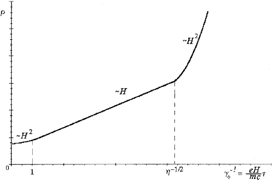
Figure 3: The dependence of the transverse resistance ($\boldsymbol{H}\bot\boldsymbol{j}$) along the normal to the layers on a magnetic field.

For $\eta^{1/2}<\gamma_{0}\ll 1$ the free path time is not contained in the asymptotic expression for the magnetoresistance, and the problem of the collision integral does not arise. When it is possible to obtain more perfect single crystals of the high-temperature metal-oxide conductors, for which the condition of the strong magnetic field can be satisfied, then at $\boldsymbol{H}\bot\boldsymbol{j}$ the linear growth with $H$ of their magnetoresistance will be expected (Fig. 3).

3. PROPAGATION OF ELECTROMAGNETIC WAVES IN
LAYERED CONDUCTORS

The depth of penetration of an electromagnetic wave into the layered conductor with the quasi-two-dimensional electron energy spectrum depends essentially on the polarization of the incident wave. A linearly polarized wave whose electric field is aligned with the normal to the layers can penetrate a priori to a greater depth than a wave with the electric vector coplanar with the layers. Under the normal skin-effect conditions, when the skin layer depth is much more than the charge carriers free path length $l$, the attenuation depth $\delta_{\|}$ for the electric field $E_{z}(\boldsymbol{r})$ is $1/\eta$ times greater than the skin depth $\delta_{\bot}$ for the electric field along the layers

$$\delta_{\bot}=\delta_{\|}\eta.$$ (3.1)

In the case of the anomalous skin effect, when the skin layer depth $\delta_{\|}$ is much less than $l$, the relation between $\delta_{\bot}$ and $\delta_{\|}$ has the form

$$\delta_{\bot}=\delta_{\|}\eta^{3/2}.$$ (3.2)

In a magnetic field, especially under the anomalous skin-effect conditions, the relations between $\delta_{\bot}$ and $\delta_{\|}$ are more variable.

We consider the propagation of electromagnetic waves in the half space $x\geq 0$ occupied by the layered conductor in a magnetic field $\boldsymbol{H}=(H\sin\phi,H\cos\phi\sin\theta,H\cos\phi\cos\theta)$, where $\phi$ is the angle of deviation of a magnetic field from the sample surface $x_{\rm s}=0$.

The complete set of equations representing the problem consists of the Maxwell equations

$$(\nabla\times\boldsymbol{H}) = -i\omega\boldsymbol{E}+\frac{4\pi\boldsymbol{j}}{c};$$ (3.3)

$$(\nabla\times\boldsymbol{E}) = i\omega\boldsymbol{B};$$

$$\boldsymbol{B} = \boldsymbol{H}+4\pi\boldsymbol{M};$$ (3.4)

and the kinetic equation for the charge carriers distribution function $f(\boldsymbol{p},x,t)=f_{0}(\varepsilon)-\psi(\boldsymbol{p},x)\exp\{-i\omega t\}\partial f_{0}(\varepsilon)/\partial\varepsilon$:

$$v_{x}\frac{\partial\psi}{\partial x}+\frac{e}{c}(\boldsymbol{v}\times\boldsymbol{H})\frac{\partial\psi}{\partial\boldsymbol{p}}+\left(\frac{1}{\tau}-i\omega\right)\psi=e\boldsymbol{vE}(x);$$ (3.5)

the solution of which allows us to determine the relation between the current density and the electric field of the wave.

Here $\boldsymbol{M}$ is the magnetization of a conductor. Usually the magnetic susceptibility $\chi_{ij}=\partial M_{i}/\partial B_{j}$ of nonmagnetic conductors is negligible, and below we shall not distinguish between the magnetic field and the magnetic induction $\boldsymbol{B}$, except for some special cases, when the de Haas–van Alfven effect is most pronounced and results in the appearance of diamagnetic domains [24, 25]. The perturbation of the charge carriers system caused by the electromagnetic wave is supposed to be sufficiently weak, and here we confine our consideration to a linear approximation in a weak electric field. The Maxwell equations in this approximation become linear and we can also suppose the electromagnetic wave to be monochromatic with the frequency $\omega$, without loss of the generality. This follows from the fact that the solution of the problem in the case of an arbitrary time-dependence of the fields presents the superposition of the solutions for different harmonics. For this reason the time differentiation in the Maxwell equations (3.3) and (3.4) is equivalent to multiplication by $(-i\omega t)$. Below $t$ will indicate the time of the charge motion in a magnetic field according to Equations (2.9).

The kinetic equation (3.5) should be supplemented with the boundary condition allowing for the scattering of charge carriers by the sample surface $x_{\rm s}=0$

$$\psi(\boldsymbol{p}_{+},0) = q(\boldsymbol{p}_{-})\psi(\boldsymbol{p}_{-},0)$$ (3.6)

$$\times \int\mbox{d}^{3}p\,W(\boldsymbol{p},\boldsymbol{p}_{+})\{1-\Theta[v_{x}(\boldsymbol{p})]\}\psi(\boldsymbol{p},0);$$

where the sample surface specularity parameter $q(\boldsymbol{p})$ is the probability for a conduction electron incident onto the surface $x_{\rm s}=0$ to be reflected specularly with momentum $\boldsymbol{p}$. The specularity parameter is related to the scattering indicatrix $W(\boldsymbol{p},\boldsymbol{p}_{+})$ through the expression

$$q(\boldsymbol{p}_{-})=1-\int\mbox{d}^{3}p\,W(\boldsymbol{p},\boldsymbol{p}_{+})\{1-\Theta[v_{x}(\boldsymbol{p})]\};$$ (3.7)

$\Theta(\zeta)$ is the Heaviside function and the momenta $\boldsymbol{p}_{-}$ and $\boldsymbol{p}_{+}$ (of incident and scattered electrons, respectively) are related by the specular reflection condition, which conserves energy and momentum projection on the sample surface.

The integral term in the boundary condition (3.6) ensures no current through the surface. However, in the range of high frequencies $\omega$ the solution to the kinetic equation depends weakly on this functional of the scattering indicatrix and, without reference to it, has the form

$$\psi(t_{\rm H},p_{\rm H},x) = \int\limits_{\lambda}^{t_{\rm H}}\mbox{d}t\,e\boldsymbol{v}(t,p_{\rm H})\boldsymbol{E}(x(t,p_{\rm H})-x(\lambda,p_{\rm H}))$$ (3.8)

$$\times \exp\{\nu(t-t_{\rm H})\}+\frac{q(\lambda,p_{\rm H})}{1-q(\lambda,p_{\rm H})\exp\{\nu(2\lambda-T)\}}$$

$$\times \int\limits_{\lambda}^{T-\lambda}\mbox{d}t\,e\boldsymbol{v}(t,p_{\rm H})\boldsymbol{E}(x(t,p_{\rm H})-x(\lambda,p_{\rm H}))$$

$$\times \exp\{\nu(t-t_{\rm H}+2\lambda-T)\};$$

where $\nu=-i\omega+1/\tau$, and $\lambda$ is the nearest to $t_{\rm H}$ root of the equation

$$x(t,p_{\rm H})-x(\lambda,p_{\rm H})=\int\limits_{\lambda}^{t}v_{x}(t^{\prime},p_{\rm H})\,\mbox{d}t^{\prime}=x;$$ (3.9)

For electrons that do not collide with the specimen boundary, i.e. at $\{x(t_{\rm H},p_{\rm H})-x_{\rm min}\}<x$, one should put $\lambda=-\infty$.

After several collisions with the surface $x_{\rm s}=0$ in an oblique magnetic field electrons either move into the bulk of the conductor or tend to approach the surface. The relative number of electrons is not large and they do not contribute markedly to an alternating current at $\phi\cong 1$. The contribution of the remaining electrons, naturally, depends on the nature of their interaction with the surface, but the state of the surface influences unessential numerical factors of the order of unity in the expression for the surface impedance.

Following Reuter and Sondheimer [26], we continue the electric field and the current density in an even manner to the region of negative values of $x$, and apply a Fourier transformation, viz.

$$\boldsymbol{E}(k) = 2\int\limits_{0}^{\infty}\mbox{d}x\,\boldsymbol{E}(x)\cos kx;$$

$$\boldsymbol{j}(k) = 2\int\limits_{0}^{\infty}\mbox{d}x\,\boldsymbol{j}(x)\cos kx.$$ (3.10)

As a result, the Maxwell equations after the exclusion of the magnetic field of the wave takes the form

$$\left\{k^{2}-\frac{\omega^{2}}{c^{2}}\right\}E_{\alpha}(k)-\frac{4\pi i\omega j_{\alpha}(k)}{c^{2}}=-2E_{\alpha}^{\prime}(0);\quad\alpha=(y,z),$$ (3.11)

where the prime denotes differentiation with respect to $x$.

The solution of the kinetic equation (3.8) allows us to find the relation between the Fourier transforms of the electric field and the current density.

$$j_{i}(k)=\sigma_{ij}(k)E_{j}(k)+\int\mbox{d}k^{\prime}\,Q_{ij}(k,k^{\prime})E_{j}(k^{\prime});$$ (3.12)

where

$$\sigma_{ij}(k) = \frac{2e^{3}H}{c(2\pi\hbar)^{3}}\int\mbox{d}p_{\rm H}\int\limits_{0}^{T}\mbox{d}t\,v_{i}(t,p_{\rm H})\int\limits_{-\infty}^{t}\mbox{d}t^{\prime}\,v_{j}(t^{\prime},p_{\rm H})$$ (3.13)

$$\times \exp\{\nu(t^{\prime}-t)\}\cos k\{x(t^{\prime},p_{\rm H})-x(t,p_{\rm H})\}$$

$$\equiv \langle e^{2}v_{i}{\hat{R}}v_{j}\rangle.$$

The kernel of the integral operator $Q_{ij}$ depends essentially on the condition of the specimen surface, i.e. on the probability of the specular reflection of charge carriers.

The electric field $E_{x}(x)$ should be determined from the Poisson equation

$$\mbox{div}\,\boldsymbol{E}=4\pi e\langle\psi\rangle,$$ (3.14)

which in conductors with a high charge carriers density reduces to the condition of electrical neutrality of a conductor

$$\langle\psi\rangle=0.$$ (3.15)

The condition of charge conservation, following from the continuity equation

$$-i\omega e\langle\psi\rangle+\mbox{div}\,\boldsymbol{j}=0;$$ (3.16)

and the macroscopic boundary condition (the absence of the current through the surface $x_{\rm s}=0$) enable us to relate the electric field $E_{x}(x)$ with the other components of the field. The equality to zero of the current $j_{x}$ for any $x$,

$$j_{x}(k)=\sigma_{xx}(k)E_{x}(k)+\sigma_{x\alpha}(k)E_{\alpha}(k)=0;\quad\alpha=(y,z),$$ (3.17)

together with the Equation (3.11) allows us to find the Fourier-transform $\boldsymbol{E}(k)$, and then, by using the inverse Fourier transformation, to obtain the distribution of the electric field in the conductor

$$E_{\alpha}(x)=\frac{1}{2\pi}\int\limits_{0}^{\infty}\mbox{d}k\,E_{\alpha}(k)\exp\{-ikx\}.$$ (3.18)

3.1 Normal Skin Effect

The penetration of an electromagnetic field into the conductor under the following conditions: when the current density $\boldsymbol{j}(\boldsymbol{r})$ is determined by the value of the electric field $\boldsymbol{E}(\boldsymbol{r})$ in the same point $\boldsymbol{r}$, is known as the normal skin effect.

In the absence of open electron orbits, the high-frequency current may be produced mainly by conduction electrons that are removed from the surface at greater distance than the electron orbit diameter and do not collide with the sample surface. This takes place in sufficiently strong magnetic fields parallel to the sample surface ($\phi=0$) when the curvature radius $r$ of the charge carriers trajectory is much less than the skin-layer depth. In this case the relation between the current density and the electric field can be treated as local, as in the case of the normal skin-effect, although we may take any proportion between $l$ and $\delta$.

The depth of the skin-layer is determined by the roots of the dispersion equation

$$\mbox{det}\,\left\{\left(k^{2}-\frac{\omega^{2}}{c^{2}}\right)-\frac{4\pi i\omega}{c^{2}}{\tilde{\sigma}}_{\alpha\beta}(k)\right\}=0,$$ (3.19)

where

$${\tilde{\sigma}}_{\alpha\beta}(k)=\sigma_{\alpha\beta}(k)-\frac{\sigma_{\alpha x}(k)\sigma_{x\beta}(k)}{\sigma_{xx}(k)};\quad\alpha,\beta=(y,z).$$ (3.20)

At $kr\ll 1$ the asymptotic expression for $\sigma_{ij}(k)$ is of the same form as that in a uniform electric field, hence $\sigma_{zz}$ can be described by Equations (2.31)–(2.33), where the frequency of collisions $1/\tau$ should be replaced by $\nu$. In a strong magnetic field the asymptotic value of $\sigma_{yy}$ is proportional to $\sigma_{0}(\eta\tan\theta)^{2}$, because ${\bar{v}}_{y}={\bar{v}}_{z}\tan\theta$. However, in this approximation the Hall field is large and ${\tilde{\sigma}}_{zz}$ is of the order of $\sigma_{0}$ ($\sigma_{0}$ is the conductivity in the layers-plane at $H=0$ in an uniform electric field). As a result, at $kr\ll 1$ the electric field $E_{y}$ attenuates at distance

$$\delta_{\bot}\cong\delta_{0}=c(2\pi\omega\sigma_{0})^{-1/2}$$ (3.21)

for any proportion between the free path length and the skin-layer depth.

At $\eta\ll 1$ each of the components $\sigma_{zx}$ and $\sigma_{xz}$ is proportional to $\eta^{2}$ or to higher powers of $\eta$, so that ${\tilde{\sigma}}_{zz}\cong\sigma_{zz}$. For small $\theta$ the asymptotic value of $\sigma_{zz}(k)$ is about $\sigma_{0}\eta^{2}$ and the depth $\delta_{\|}$ is $1/\eta$ times greater than $\delta_{\bot}$ (as for normal skin effect conditions), if the Fermi surface corrugation is not too small and $\eta\geq\delta_{0}\omega/c$. At $\omega\gg\sigma_{0}\eta^{2}$ and $\eta r\leq\delta_{0}$ the skin-layer depth

$$\delta_{\|}=\frac{\delta_{0}^{2}\omega}{c}\left(1+\frac{r^{2}\omega^{2}}{c^{2}}\right)^{-1/2}$$ (3.22)

increases with increasing magnetic field and attains the value $\omega\delta_{0}^{2}/c$.

When $\theta$ is not small, there is a sequence of values $\theta=\theta_{\rm c}$, at which the asymptotic behaviour of $\sigma_{zz}$, (and hence of ${\tilde{\sigma}}_{zz}$) changes essentially. For $\tan\theta\gg 1$ this sequence repeats periodically but the period as well as the values $\theta_{\rm c}$ differ slightly from those in the case of static fields. This results from the fact that the stationary phase points $\boldsymbol{kv}=\omega$ do not coincide with the turning points on an electron orbit where $v_{x}$ disappears. However the phase velocity of the wave $v_{\phi}=\omega/k=(\omega\tau)^{-1/2}\omega c/\omega_{0}\eta$ is much less than the Fermi velocity $v_{\rm F}$, hence the period of changing of the asymptotic value of ${\tilde{\sigma}}_{zz}(k,\theta)$ is determined, to a good accuracy, by the Fermi surface diameter and has the form (2.35). At $\theta=\theta_{\rm c}$ the asymptotic value for $\sigma_{zz}$ decreases significantly for small $\eta$, $\gamma=(\Omega_{0}\tau\cos\theta)^{-1}$, $\omega/\Omega_{0}$ and $kr$, viz.

$${\tilde{\sigma}}_{zz}(k,\eta,\theta_{\rm c})=\sigma_{0}\eta^{2}\{\eta^{2}f_{1}(\theta_{\rm c})+\gamma^{2}f_{2}(\theta_{\rm c})+(kr)^{2}f_{3}(\theta_{\rm c})\},$$ (3.23)

where $f_{i}$ are the functions of $\theta$ of the order of unity.

The penetration depth for the electric field $E_{z}$ grows substantially for $\theta=\theta_{\rm c}$. In the angular dependence of the impedance there is a series of narrow spikes at $\theta=\theta_{\rm c}$, which in pure conductors ($l\eta^{2}>\delta_{0}$) diminish with increasing magnetic field, whereas at $l\eta^{2}<\delta_{0}$ they grow proportionally to $l\delta_{0}/r\eta$ if $l\eta<r<\delta_{0}/\eta$. At certain frequencies (not too high sufficiently), when the displacement current is small compared to the conduction current the solution of the dispersion equation (3.19) at $\theta=\theta_{\rm c}$ can be represented by the following interpolation formula

$$\delta_{\|}=l\left(\frac{r^{2}+\delta_{0}^{2}\eta^{-2}}{r^{2}+l^{2}\eta^{2}}\right)^{1/2}.$$ (3.24)

In the case of low electrical conductivity across the layers, when the condition $\omega/c>\sigma_{0}\eta^{2}(\eta^{2}+r^{2}/l^{2})$ is met, the skin depth $\delta_{\|}$ has the form

$$\delta_{\|}=\frac{\delta_{0}}{\eta^{2}}\left\{1+\left(\frac{r}{l\eta}\right)^{2}+\left(\frac{r\omega}{c\eta}\right)^{2}\right\}^{-1/2}\left\{1+\left(\frac{r\eta}{\delta_{0}}\right)^{2}\right\},$$ (3.25)

and in a strong magnetic field, when $r<(l^{2}\eta^{2}+\delta_{0}^{2}/\eta^{2})^{1/2}$, the electric field decay length across the layers is again $\delta_{0}/\eta^{2}$. In the region of sufficiently strong magnetic fields, when at $\theta=\theta_{\rm c}$ the relation $\delta_{0}/\eta\ll r\ll\delta_{\|}$ is valid, the impedance as a function of a magnetic field has a minimum value because for $r\gg l\eta$ the skin depth

$$\delta_{\|}=l\frac{r\eta}{\delta_{0}}$$ (3.26)

is inversely proportional to the magnetic field magnitude [27, 28].

At $\delta_{\bot}\ll r\ll\delta_{\|}$ the decay length pertaining to the electric field $E_{z}(x)$ is, as before, weakly dependent on the character of charge carriers interaction with the conductor surface, whereas the penetration depth for the electric field $E_{y}(x)$ is very sensitive to the state of the surface if $\delta_{\bot}$ is less or comparable with the charge carriers mean free path. In this range of magnetic fields the normal skin effect is realizable only for $\delta_{\bot}\gg l$, when the local connection between the current density and the electric field takes place at an arbitrary orientation of the magnetic field. Asymptotic expression for ${\tilde{\sigma}}_{yy}(k)$ at $kl\ll 1$ coincides with $\sigma_{0}$ up to numerical factor of the order unity and, hence, $\delta_{\bot}$ is of the same order of magnitude as $\delta_{0}$. However, the penetration depth for the electric field $E_{z}(x)$ depends essentially on the orientation of the magnetic field. The solution of the dispersion equation (3.19) has the form

$$k = \frac{(2\pi\omega)^{1/2}(1+i)}{2c}\Biggl{\{}\sigma_{0}^{-1}+\sigma_{zz}^{-1}$$ (3.27)

$$\pm \left[(\sigma_{zz}^{-1}-\sigma_{0}^{-1})^{2}-\left(\frac{2H\sin\theta\sin\phi}{Nec}\right)^{2}\right]^{1/2}\Biggr{\}}^{-1/2}.$$

Inessential numerical factors of the order of unity depending on the concrete form of the electron energy spectrum are omitted in Equation (3.27). When $\theta$ differs essentially from $\pi.2$, in an extremely strong magnetic field ($\gamma\ll\eta^{2}$) the propagation of helical waves is possible. For $\phi\cong 1$ one of the roots of the dispersion equation describes the attenuation of the electric field along the layers at distances of the order of

$$\delta_{\bot}=\delta_{0}\left\{1+\frac{\sigma_{zz}}{\sigma_{0}\gamma^{2}}\right\}^{1/2}.$$ (3.28)

It is easily seen that the depth of penetration for the field $E_{y}$ grow proportionally to $H$, when $\gamma\ll\eta$. At $\gamma\gg\eta^{2}$ the electric field along the normal attenuates at distances

$$\delta_{\|}=\delta_{0}\left(\frac{\sigma_{0}}{\sigma_{zz}}\right)^{1/2},$$ (3.29)

i.e. at distances of the order of $\delta_{0}/\eta$, as in the absence of a magnetic field.

The specific dependence of the attenuation length for the field $E_{z}(x)$ takes place at $\theta=\pi/2$, when, apart from the charge carriers drift along $\boldsymbol{H}$-direction, in the $xy$-plane there are many possible directions of drift for charge carriers belonging to open Fermi surface cross-sections. In this case the dependence of $\sigma_{zz}$ on the magnitude of a strong magnetic field ($\gamma_{0}\ll 1$), given by the following interpolation expression

$$\sigma_{zz}=\sigma_{0}\gamma_{0}^{2}\eta^{2}(\gamma_{0}^{2}+\eta)^{-1/2},$$ (3.30)

is the same for any orientation of a magnetic field in the $xy$-plane.

Using Equations (3.29) and (3.30), it is easy to demonstrate that at $\eta^{1/2}\ll\gamma_{0}\ll 1$ the attenuation length $\delta_{\|}$ increases with increasing magnetic field as $H^{1/2}$, and at $\eta^{2}\ll\gamma_{0}\leq\eta^{1/2}$ the length of electric field attenuation along the normal to the layers $\delta_{\|}\cong\delta_{0}/\gamma_{0}\eta^{3/4}$ grows linearly with a magnetic field.

3.2 Anomalous Skin Effect

When the frequency of the electromagnetic wave increases, a local connection between the current density and the electric field $E_{y}(x)$ may be broken and the Maxwell equations appear to be integral even in the Fourier representation. In the presence of a magnetic field a strict solution of the problem has been suggested by Hartmann and Luttinger for some special cases [29]. If the numerical factors of the order of unity are not used, the dependencies of the surface impedance and other characteristics of waves on physical parameters can be obtained by means of the correct estimation of the contribution given by the integral term in Equation (3.12) to the Fourier transform of the high-frequency current. In a magnetic field applied parallel to the sample surface, the contribution to the current from charge carriers colliding with the surface is essential at $\delta_{\bot}\leq r$. When the reflection of charge carriers at the specimen boundary is close to specular (the width of the scattering indicatrix $w$ is much less than $r^{3/2}/l\delta_{\bot}^{1/2}$), the contribution to the high-frequency current from electrons “slipping” along the sample surface is great and the asymptotic expression for ${\tilde{\sigma}}_{yy}(k)$ at large $k$ has the form

$${\tilde{\sigma}}_{yy}(k)=\frac{\omega_{0}^{2}}{\Omega(kr)^{1/2}(w+r/l)}.$$ (3.31)

By means of the dispersion equation (3.19) the length of electric fields decay can be easily determined

$$\delta_{\bot}=\delta_{0}^{6/5}r^{-1/5}\left(w+\frac{r}{l}\right)^{2/5};\quad\delta_{\|}=\frac{\delta_{0}}{\eta}.$$ (3.32)

In this region of weak magnetic fields ($\delta_{\bot}\ll r\ll l$) the impedance has a minimum at $r=wl$, the width of the scattering indicatrix being determined by the position of the minimum.

In a magnetic field applied parallel to the sample surface under the conditions of anomalous skin-effect, when the skin depth is the smallest length parameter, i.e. both $\delta_{\bot}$, and $\delta_{\|}$ are much less than $r$ and $l$, the universal relation between $\delta_{\bot}$ and $\delta_{\|}$ takes place at $w\ll r^{3/2}/l\delta_{\|}^{1/2}$, viz.

$$\delta_{\bot}=\delta_{\|}\eta^{4/5}.$$ (3.33)

If $w\gg r^{3/2}/l\delta_{\bot}^{1/2}$ and $\delta_{\bot}\ll r\ll l$, the high-frequency current is produced mainly by charge carriers that do not collide with the sample surface and the relation between $\delta_{\bot}$ and $\delta_{\|}$ has the form (3.2).

In the intermediate case, when $r^{3/2}/l\delta_{\|}^{1/2}\ll w\ll r^{3/2}/l\delta_{\bot}^{1/2}$, only $\delta_{\bot}$ is essentially dependent on $w$ for $w\geq r/l$:

$$\delta_{\|} = r^{1/3}\left(\frac{\delta_{0}}{\eta}\right)^{2/3};$$

$$\delta_{\bot} = (wl)^{2/5}\delta_{0}^{4/5}r^{-1/5}.$$ (3.34)

In the absence of open electron orbits the information on the skin-layer field can be electronically transported deeper into the conductor in the form of narrow field spikes, predicted by Azbel’ [30]. The electron transport of the electromagnetic field and the screening of the incident wave at the surface $x_{\rm s}=0$ is due mainly to the charge carriers that are in phase with the wave and move nearly parallel to the sample surface. At $\eta\leq\delta/r$ field spikes are produced with the participation of almost all charge carriers [31]. Without reference to collisions, the intensities of the spikes at distances, that are multiples of the electron orbit diameter along the $x$ axis, are in the same range. Allowance for the scattering of conduction electrons in the bulk of a conductor, results in the attenuation of the field in the spikes at distance of the order of the mean free path. Thus under the anomalous skin effect conditions there are two scale lengths of wave decay. Apart from the damping effect over the skin depth the electromagnetic field penetrates into the conductor to distances of the order of the mean free path $l$.

In the case when $\eta\gg\delta/r$, spike formation is provided by a small fraction of order $(\delta/r\eta)^{1/2}$ of the charge carriers whose orbit diameter scatter near the extremal section is comparable to the skin layer depth. As a result, the spike intensities decrease as the distance from the face $x_{\rm s}=0$ increases, and apart from the factor $\exp\{-x/l\}$ every subsequent spike acquires the small factor $(\delta/r\eta)^{1/2}$.

While the angle $\theta$ approaches $\pi/2$, closed electron orbits become strongly elongated in the $x$-direction. When the orbit diameter along the $x$-axis exceeds the free path length $l$, the spike mechanism of the electromagnetic field penetration into the conductor is replaced by the electron transport of the field in the form of Reuter–Sondheimer quasi-waves.

3.3 Weakly Damping Reuter–Sondheimer Waves

Consider the electron transport of the electromagnetic field at $\theta=\pi/2$. In order to find the field in a depth of the conductor by means of the inverse Fourier transformation (3.18) we continue $\sigma_{ij}(k)$ analytically into the whole complex $k$-plane and supplement the integration contour with an arc of an infinitely large radius. The skin layer depth is determined by poles of the integrand in Equation (3.18), whereas weakly attenuated waves are connected to the integration along the cut-line drawn from the branching point of the function $E_{j}(k)$. It can be easily seen that at however small $\eta$ the components of the tensor $\sigma_{ij}(k)$ has a power $1/2$ singularity:

$$\sigma_{zz}(k) = \frac{\omega_{0}^{2}\eta^{2}}{\nu}\{(\alpha_{+}^{2}-1)^{-1/2}+(\alpha_{-}^{2}-1)^{-1/2}\};$$ (3.35)

$$\Delta\sigma_{yy}(k) = \nu\left(\frac{\omega_{0}}{kv}\right)^{2}\left\{\left(\frac{kv}{\nu}\right)^{2}+1\right\}^{1/2},$$ (3.36)

where $\omega_{0}$ is the plasma frequency, $\alpha_{\pm}=i(kv\pm\Omega_{0})/\nu$ unessential numerical factors of the order of unity are omitted.

The kernel of the integral operator $Q_{ij}(k,k^{\prime})$ as a function of $k$ has such a singularity as well.

At distances from the sample surface that are greater than either the curvature radius of the electron trajectory $r=v/\Omega_{0}$ or the electron displacement $2\pi v/\omega$ per period of the wave the electromagnetic field decreases proportionally to $x^{-3/2}\exp(-x/l)$. For $\Omega_{0}\gg\omega$ the slowly decreasing electric field $E_{z}(x)$ oscillates with $H$ at large $x$:

$$E_{z}(x) = E_{z}(0)\eta^{-4/3}\left(\frac{\omega_{0}}{c}\right)^{4/3}\left(\frac{v}{\omega}\right)^{2/3}r^{-1/2}x^{-3/2}$$ (3.37)

$$\times \exp\left\{\frac{ix}{r}-\frac{x}{l}\right\};\quad r\ll x\ll\frac{r}{\eta}.$$

At $\eta\ll 1$ the attenuation of the electric field $E_{y}(x)$ over the charge carriers free path length has the form

$$E_{y}(x)=E_{y}(0)\left(\frac{\omega_{0}}{c}\right)^{4/3}\left(\frac{v}{\omega}\right)^{2/3}x^{-3/2}\exp\left\{-\frac{x}{l}\right\};\quad\frac{v}{\omega}\ll x\ll\frac{v}{\omega\eta},$$ (3.38)

and does not contain the magnetic field magnitude.

The oscillatory dependence of $E_{y}(x)$ upon the magnetic field magnitude occurs only in the case, when the charge with velocity $v_{y}$ is not an integral of motion, and manifests itself in small corrections proportional to $\eta^{2}$. Numerical factors of order unity, being dependent on the concrete form of the electron dispersion law, are omitted in Equations (3.37) and (3.38).

In a sufficiently strong magnetic field ($r\ll l\eta$) the asymptotic behaviour of the weakly damping field $E_{z}(x)$ changes essentially with displacement from the sample surface. In the absence of a magnetic field $\sigma_{yy}(k)$ and $\sigma_{zz}(k)$ have logarithmic singularities at $k_{1}=i\nu/v_{1}$ and $k_{2}=i\nu/v_{2}$, except were $\eta$ is not small. $v_{1}$ is the electron velocity in the reference point (in the $x$-direction) of the Fermi surface and $v_{2}$ is the velocity projection $v_{x}$ in the Fermi surface saddle point, where the connectivity of the line $v_{x}=\mbox{const}$ changes [32]. At small values of $\eta$ these branching points for the components of the high-frequency conductivity tensor approach each other, and at $\eta=0$ the logarithmic singularity is replaced by the power $1/2$ singularity of the form (3.35), (3.36). Let the integration contour in the $k$-plane at small $\eta$ be drawn along the cut-line from the branching points $k_{1}$ and $k_{2}$ parallel to the imaginary axis, to go round both branching points. Then the electric field $E_{z}(x)$ at large distances from the skin layer takes the following form.

$$E_{z}(x) = \int\limits_{k_{1}}^{k_{1}+i\infty}\frac{\mbox{d}k\,\exp(ikx)}{k^{2}-\omega^{2}/c^{2}-4\pi i\omega c^{-2}\sigma_{zz1}(k)}$$ (3.39)

$$+ \int\limits_{k_{2}}^{k_{2}+i\infty}\frac{\mbox{d}k\,\exp(ikx)}{k^{2}-\omega^{2}/c^{2}-4\pi i\omega c^{-2}\sigma_{zz2}(k)}$$

The integral along the line connecting the branching points $k_{1}$ and $k_{2}$ may be neglected; $\sigma_{zz1}(k)$ is the value of the function $\sigma_{zz}$ on the left side of the cut-line drawn from the point $k_{1}$, $\sigma_{zz1}$ is the value on the right side of the cut-line from the point $k_{2}$. $v_{1}$ is assumed to be larger than $v_{2}$. Making use of the dispersion law (2.21), we obtain the following expressions for the diagonal components of the high-frequency conductivity tensor at $k_{1}\leq k\leq k_{2}$

$$\sigma_{yy}(k) = \frac{\omega_{0}^{2}\eta}{\pi^{3}}\int\limits_{0}^{\pi}\mbox{d}\alpha\,\int\limits_{0}^{\pi/2}\frac{\mbox{d}\phi\,\sin^{2}\phi}{\nu+ikv\cos\phi(1+\eta\cos\alpha)^{1/2}};$$ (3.40)

$$\sigma_{yy}(k) = \frac{\omega_{0}^{2}\eta}{\pi^{3}}\int\limits_{0}^{\pi}\mbox{d}\alpha\,\sin^{2}\alpha\,\int\limits_{0}^{\pi/2}\frac{\mbox{d}\phi}{\nu+ikv\cos\phi(1+\eta\cos\alpha)^{1/2}};$$

It is easily seen that at $\eta=0$ the component of the high-frequency conductivity $\sigma_{zz}(k)$ is proportional to $(\nu+ikv)^{-1/2}$ and $\sigma_{yy}(k)$ is proportional to $(\nu+ikv)^{1/2}$, i.e. at $k=i\nu/v$ both of them have the power $1/2$ singularity,. When the Fermi surface corrugation is not small ($\eta\cong 1$) instead of the power $1/2$ singularity the logarithmic singularity appears for $k=i\nu/v(1+\eta)^{1/2}$ and $k=i\nu/v(1-\eta)^{1/2}$. The integral with respect to $\phi$ has the power $1/2$ singularity at $k=i\nu/v(1+\eta\cos\alpha)^{1/2}$. Interchanging the order of integration with respect to $\alpha$ and $k$ in Equation (3.39), we obtain the following expression for the weakly damping component of the electric field at large distances from the skin layer

$$E_{y}(x) = E_{y}(0)\left(\frac{c}{\omega_{0}}\right)^{4/3}\left(\frac{v}{\omega}\right)^{2/3}x^{-3/2}\left(\frac{\nu}{v}\right)^{1/2}$$ (3.42)

$$\times \int\limits_{0}^{\pi}\mbox{d}\alpha\,\exp\left\{-\frac{\nu x}{v(1+\eta\cos\alpha)^{1/2}}\right\}$$

At great distances from the sample surface the electric field along the normal to the layers can be described by the same formula, if the additional factor $\eta^{-4/3}\sin^{2}\alpha$ is written in the integral over $\alpha$. At $x\gg v/\omega\eta$ the integrand in Equation (3.42) is a rapidly oscillating function and the major contribution to the integral is given by the small vicinities near the stationary phase points $\alpha=(0,\pi)$. After simple calculations we have

$$E_{y}(x) = E_{y}(0)\left(\frac{c}{\omega_{0}}\right)^{4/3}\left(\frac{v}{\omega}\right)^{2/3}x^{-2}\eta^{-1/2}$$ (3.43)

$$\times \left[\exp\left\{-\frac{\nu x}{v(1+\eta)^{1/2}}+\right\}\exp\left\{-\frac{\nu x}{v(1-\eta)^{1/2}}\right\}\right];$$

$$x\gg\frac{v}{\omega\eta}.$$

In the formulas given above unessential numerical factors of order unity are omitted. The factor at the exponent in Equation (3.43) is inversely proportional to $x^{2}$, as in ordinary metals. Such asymptotic behaviour of the electric field in the layered conductors takes place only in the range of large frequencies when $\omega\tau\gg 1/\eta$. The difference in asymptotic behaviour of the electric fields at such frequencies can be understood by watching the wave phase, which is carried away from the skin layer by conduction electrons with different velocity projections $v_{x}$. At a moment $t$ and a distance $x$ electrons carry information on the electromagnetic wave whose phase is late for the quantity $\omega\Delta t=\omega x/v_{x}$. After averaging over different values of $v_{x}$ we have

$$\boldsymbol{E}(x)=\int\mbox{d}v_{x}\,\exp\left\{-i\omega t+\frac{i\omega x}{v_{x}}\right\}.$$ (3.44)

It can be easily seen that the slowly damping wave, propagating with the velocity of electrons from the Fermi surface reference point $v_{1}$, is formed by charge carriers whose velocity $v_{x}$ differs from $v_{1}$, by the quantity $\Delta v_{x}\leq v_{1}^{2}/\omega x$. If $v_{1}-v_{2}\cong v\eta$ is less than $\Delta v_{x}$, i.e. $x\leq v\omega\eta$, then Equation (3.38) takes place, and in the opposite case, when $\Delta v_{x}\ll v\eta$, electrons from the small vicinity of the Fermi surface saddle and reference points produce weakly damping waves of the form (3.43).

In a magnetic field, the charge carriers that belong to one of the sides of the central open Fermi surface cross section, (at which the velocity $v_{x}$ alters periodically with time in the interval between $v_{2}$ and $v_{1}$) move more rapidly into the bulk of the sample. The weakly damping waves propagate with velocity, equal to the extremal value ${\bar{v}}_{x}$, and can be described by Equations (3.37) and (3.38).

Weakly damping waves are of the analogous form, in a magnetic field $\boldsymbol{H}=(H\cos\phi,H\sin\phi\cos\theta,H\sin\phi\cos\theta)$ deflected from the layers-plane. If ??? and $\phi$ differ from zero essentially, the weakly damping wave at $\theta=\pi/2$ propagates with velocity ${\bar{v}}_{x}$, which is equal to the velocity of drift for charge carriers on the open Fermi surface cross-section containing the reference point with respect to the axis $p_{x}$. The asymptotic behaviour of the electric field $E_{y}(x)$ can be described by Equation (3.38), and the oscillatory dependence on the magnetic field, applied orthogonal to the axis of the corrugated cylinder, manifests itself, as before, only in small corrections proportional to $\eta^{2}$. However at $\phi\ll 1$ and $\theta=\pi/2$ the asymptotic behaviour of $E_{z}(x)$ and $E_{y}(x)$ at great distances from the sample surface can change essentially.

In a magnetic field applied orthogonal to the surface ($\phi=0$) the electrons with closed orbits and also a considerable part of charge carriers on open orbits near the self-intersecting orbit, participate in the formation of the weakly damping waves at distances $x\ll v/\omega\eta$. If the charge carriers dispersion law used is, as before, Equation (2.21), $\sigma_{ij}(k)$ takes the form

$$\sigma_{ij}(k)=\frac{2e^{2}}{(2\pi h)^{3}}\sum\limits_{n}\int\mbox{d}p_{x}\,2\pi m^{*}\frac{v_{i}^{-n}v_{j}^{n}}{\nu+ikv_{x}+in\Omega}.$$ (3.45)

At a distance $x\gg v/\omega\eta$ the faster wave is formed by charge carriers with the closed orbit near the Fermi surface reference point and the factor at the exponent in the asymptotic expression for the electric field decreases proportionally to $x^{2}$ with increasing $x$. If $\eta^{1/2}\ll\gamma_{0}$, i.e. an electron has no time to make a complete revolution along the orbit during the free path time, then not only the field $E_{y}$ but also the field $E_{z}$ are independent of $H$ at such great distances.

At low temperatures, when the smearing $k_{\rm B}T$ of the Fermi distribution function for charge carriers is less than the spacing between quantum energy layers $\hbar\Omega$, the magnetic susceptibility as well as other kinetic characteristics oscillates with the inverse magnetic field in the quasiclassical region. In this case the amplitude of the quantum oscillations of the magnetic susceptibility may considerably exceed the monotonically changing part and even equal the magnitude $1/4\pi$. If the sample surface coincides with a plane of symmetry for the crystal, the main axes for the magnetic susceptibility tensor, coincide with the axes $y$ and $z$ accurately. The Maxwell equations in this case take the form

$$\left\{\sigma_{yy}(k)+\frac{\omega}{4\pi i}-\frac{k^{2}c^{2}}{4\pi i\omega}(1-pi\chi_{zz})\right\}E_{y}(k)$$

$$+\sigma^{*}_{yz}(k)E_{z}(k) = -E^{\prime}_{y}(0);$$ (3.46)

$$\sigma^{*}_{zy}(k)E_{y}(k)+$$

$$\left\{\sigma^{*}_{zz}(k)+\frac{\omega}{4\pi i}-\frac{k^{2}c^{2}}{4\pi i\omega}(1-4\pi\chi_{yy})\right\}E_{z}(k) = -E^{\prime}_{z}(0),$$ (3.47)

where

$$\sigma_{\alpha\beta}^{*}(k)=\sigma_{\alpha\beta}(k)-\frac{4\pi\sigma_{\alpha x}(k)\sigma_{x\beta}(k)}{4\pi\sigma_{xx}(k)-i\omega},$$

$(\alpha,\beta)=(y,z)$.

It is easy to make sure that the oscillating part of the magnetization

$$\boldsymbol{M}_{\rm osc} = \frac{\partial}{\partial\boldsymbol{H}}\biggl{\{}2\mbox{Re}\sum\limits_{q=1}^{\infty}\frac{(-1)^{q}}{q^{2}}\frac{eH}{2\pi^{2}c(2\pi h)2}\int\mbox{d}\varepsilon\,\frac{\partial f_{0}}{\partial\varepsilon}\int\mbox{d}p_{\rm H}\,h\Omega$$ (3.48)

$$\times \exp\left(\frac{iqcS(\varepsilon,p_{\rm H})}{eHh}\right)\biggr{\}}$$

decreases with increasing $\theta$, so that the amplitude of the magnetic susceptibility is maximum for the magnetic field directed along the normal to the layers ($\theta=0$), and $M_{\rm osc}$ is proportional to $\eta$ for $\theta=\pi/2$. As a result, when the electric field of the incident wave is linearly polarized along the normal to the layers, the surface impedance undergoes small quantum oscillations with an inverse magnetic field. The electric field in the layers plane attenuates at a distance

$$\delta=\left\{\frac{vc^{2}(1-4\pi\chi)}{\omega\omega_{0}^{2}}\right\}^{1/3},$$

if $\chi=\chi_{zz}<1/4\pi$, and the impedance undergoes giant oscillations at $(1-4\pi\chi^{\rm max})\ll 1$. In the opposite case $((1-4\pi\chi^{\rm max}))<0$ homogeneous state is unstable for some values of a magnetic field which leads to the formation of magnetic domains.

The considered cases of electromagnetic waves propagation in the layered conductors with the quasi-two-dimensional electron energy spectrum prove that they possess a great variety of specific high-frequency properties, that will, undoubtedly, be used in modern electronics.

Such a strong dependence of the intensity of the wave on its polarization allows us to utilize even thin plates of layered conductors (whose thickness is much more than skin depth but less or of the order of the free path length) as filters allowing the wave to pass with a certain polarization.

4. ACOUSTIC TRANSPARENCY OF LAYERED CONDUCTORS

When acoustic waves propagate in a layered conductor placed in a magnetic field, the quasi-two dimensional nature of the charge carriers energy spectrum is expected to be pronounced. Being very sensitive to the form of electron energy spectrum, the magnetoacoustic effects [33–36] have been used successfully for restoration of the Fermi surface, and in the low-dimensional conductors they are worthy of the special examination.

In conducting crystals apart from the sound waves attenuation related to the interaction between thermic phonons and coherent phonons with the frequency $\omega$, there are many mechanisms of electron absorption of acoustic waves. The most essential of them is the so-called deformation mechanism connected with charge carriers energy renormalization under strain

$$\delta\varepsilon=\lambda_{ij}u_{ij}.$$ (4.1)

where $\lambda_{ij}$ is the deformation potential tensor.

In a magnetic field the induction mechanism connected with electromagnetic fields generated by sound waves is also essential. These fields should be derived from the Maxwell equations (3.3), (3.4) and connection of the current density with the strain tensor $u_{ij}$ and electric field

$${\tilde{\boldsymbol{E}}}=\boldsymbol{E}+\frac{(\dot{\boldsymbol{u}}\times\boldsymbol{H})}{c}+\frac{m\ddot{\boldsymbol{u}}}{e}$$ (4.2)

can be found with the aid of the solution of the Boltzman kinetic equation. The field $\tilde{\boldsymbol{E}}$ is determined in the concomitant system of axes which moves with the velocity $\dot{\boldsymbol{u}}$.

The last term in the Equation (4.2) is connected with the Stewart–Tolmen effect.

In a weakly deformed crystal the complete set of equations for this problem is suggested by Silin [37] for isotropic metals and generalized by Kontorovich [38] to the case of an arbitrary dispersion law of charge carriers. A complete set of nonlinear equations for this problem, valid for any wave intensity, was derived by Andreev and Pushkarov [39].

Together with the Maxwell equations and Boltzman kinetic equation it is necessary to consider the dynamics equation of the elasticity theory for the ionic displacement $\boldsymbol{u}$.

$$-\omega^{2}\rho u_{i}=\lambda_{ijlm}\frac{\partial u_{lm}}{\partial x_{j}}+F_{i}.$$ (4.3)

Here $\rho$ and $\lambda_{ijlm}$ are the density and elastic tensor of the crystal. The equation contains the force $\boldsymbol{F}$ applied to the lattice from the electron system excited by the acoustic wave which is taken to be monochromatic with the frequency $\omega$. If the lattice strain is small, the force is

$$F_{i}=c[\boldsymbol{jH}]_{i}+\frac{m}{e}i\omega j_{i}+\frac{\partial}{\partial x_{k}}\langle\Lambda_{ik}\psi\rangle,$$ (4.4)

where $\Lambda_{ik}(\boldsymbol{p})=\lambda_{ik}(\boldsymbol{p})-\langle\lambda_{ik}(\boldsymbol{p})\rangle/\langle 1\rangle$.

In the linear approximation of the deformation tensor the change of charge carrier dispersion law (1.1) can be described with the aid of the deformation potential $\lambda_{ij}$ whose components depend on the quasimomentum $\boldsymbol{p}$ only and coincide in order of magnitude with the characteristic energy of the electron system, viz., the Fermi energy $\varepsilon_{\rm F}$.

Confining ourselves only to the linear approximation in a weak perturbation of conduction electrons under deformation of the crystal in kinetic equation, we obtain for $\psi$ the following expression:

$$\psi=\hat{R}\{\Lambda_{ij}(\boldsymbol{p})\dot{u}_{ij}+e\tilde{\boldsymbol{E}}\boldsymbol{v}\},$$ (4.5)

where $\hat{R}$ is the resolvent of Equation (2.2) when $1/\tau\to\nu=1/\tau-i\omega$.

Let us consider an acoustic wave propagating in $x$-direction orthogonal to a magnetic field $\boldsymbol{H}=(0,H\sin\theta,H\cos\theta)$. Using the Fourier method, derive from the Maxwell equations and Equation (4.3) a set of equations for the Fourier components of the electric field $E_{i}(k)$ and ionic displacements $u_{i}(k)$:

$$\frac{4\pi i\omega}{c^{2}}j_{\alpha}(k) = k^{2}E_{\alpha}(k)-\left(\frac{\omega}{c}\right)^{2}E_{\alpha}(k),\quad\alpha=y,z$$

$$j_{x}(k) = 0,$$

$$-\omega^{2}\rho u_{i}(k) = -\lambda_{iklx}k^{2}u_{l}+\frac{im\omega}{e}j_{i}(k)+\frac{1}{c}[\boldsymbol{j}(k)\boldsymbol{H}]_{i}+ik\langle\Lambda_{ix}\psi\rangle.$$

Using the kinetic equation solution, we can conveniently express the parameters $j_{i}(k)=\langle ev_{i}\psi(k)\rangle$ and $\langle\Lambda_{ix}\psi(k)\rangle$, which characterize the system response to the acoustic wave, in the form

$$j_{i}(k) = \sigma_{ij}(k)\tilde{E}_{j}(k)+a_{ij}(k)k\omega u_{j}(k),$$

$$\langle\Lambda_{ix}\psi(k)\rangle = b_{ij}(k)\tilde{E}_{j}(k)+c_{ij}(k)k\omega u_{j}(k),$$ (4.7)

where the Fourier components of the conductivity tensor and of acousto-electronic coupling tensors are

$$\sigma_{ij}(k)=\langle e^{2}v_{i}\hat{R}v_{j}\rangle; a_{ij}(k)=\langle ev_{i}\hat{R}\Lambda_{jx}\rangle;$$

$$b_{ij}(k)=\langle e\Lambda_{ix}\hat{R}v_{j}\rangle; c_{ij}(k)=\langle\Lambda_{ix}\hat{R}\Lambda_{jx}\rangle.$$ (4.8)

By substituting Equations (4.8) into the equation set (4.6), we obtain a system of linear algebraic equations in $u_{i}(k)$ and $\tilde{E}_{i}(k)$. After the inverse Fourier transform of the solutions of the obtained equation system, the problem of the distribution of the electric and strain fields in a conductor will be solved completely.

4.1 The Rate of Sound Attenuation

The condition for the existence of nontrivial solution of the set of equations for $u_{i}(k)$ and $\tilde{E}_{i}(k)$ (which is equal to zero of the system determinant) represents the dispersion relation between the wavevector $\boldsymbol{k}$ and the frequency $\omega$. The imaginary part of the root of the dispersion equation determines the decrements of the acoustic and electromagnetic waves and the real part describes the renormalization of their velocities related to the interaction between the waves and conduction electrons.

However the sound attenuation rate can be also determined by means of the dissipation function $Q$ which is proportional to the variation with time of the entropy of a conductor [40]. Taking into account only the electron absorption of acoustic waves we have for the dissipation function

$$Q=\langle\psi\hat{W}_{\rm col}\{\psi\}\rangle;$$ (4.9)

and for the sound damping decrement

$$\Gamma=\left\langle\frac{|\psi|^{2}}{\rho u^{2}s\tau}\right\rangle,$$ (4.10)

where $s$ is the sound velocity, the collision integral is taken in the $\tau$-approximation.

In ordinary metals the electromagnetic fields generated by sound are essential in the range of strong enough magnetic fields when the radius of curvature of the electron trajectory is much less than the mean free path and also than the sound wavelength, i.e. $kr\ll 1$. If the charge carriers trajectories are bent so that

$$1\ll kr\ll kl,$$ (4.11)

the absorption of sound wave energy in a metal is determined mainly by the deformation mechanism. In low-dimensional conductors the role of electromagnetic fields generated by a sound wave turns out to be essential in a wider range of magnetic fields, including a magnetic field which satisfies the condition (4.11) [41]. In this range of magnetic fields, the energy absorption coefficient $\Gamma$ of the acoustic wave in an ordinary (quasi-isotropic) metal oscillates with variation of the reciprocal magnetic field. The amplitude of these oscillations is small compared with the slowly varying component of $\Gamma$, and the period is determined by the extreme diameter of the Fermi surface. This effect, which was predicted by Pippard [33], is associated with a periodic repetition of the conditions of absorption of the acoustic wave energy by electrons on a selected orbit, when a number of acoustic wavelengths fitting in this orbit changes by unity. Under conditions of strong anisotropy in the energy-momentum relation for charge carriers, Pippard’s oscillations are formed not by small fractions of electrons, but by almost all charge carriers on the Fermi surface. As a result, the amplitude of periodic variations of $\Gamma$ increases sharply compared with the case of quasi-isotropic metal, and these variations acquire the form of resonance peaks [42, 43].

If the acoustic wave polarization is aligned with its wavevector ($\boldsymbol{u}=(u,0,0)$) the equations system after the exclusion of $\tilde{E}_{x}$ takes the form

$$\left(\tilde{a}_{yx}k\xi+\frac{iH_{z}}{c}\right)\omega u+(\xi\sigma_{yy}-1)\tilde{E}_{y}+\xi\tilde{\sigma}_{yz}\tilde{E}_{z} = 0;$$

$$\left(\tilde{a}_{zx}k\xi+\frac{iH_{z}}{c}\right)\omega u+(\xi\sigma_{zz}-1)\tilde{E}_{z}+\xi\tilde{\sigma}_{zy}\tilde{E}_{y} = 0;$$

$$(\omega^{2}-s^{2}k^{2})\rho u+\left[ik\tilde{c}_{xx}+\frac{1}{c}(\tilde{a}_{yx}H_{z}-\tilde{a}_{zx}H_{y})k\omega u\right]$$

$$+\left[ik\tilde{b}_{xy}+\frac{1}{c}(\tilde{\sigma}_{yy}H_{z}-\tilde{\sigma}_{zy}H_{y})\tilde{E}_{y}\right]$$

$$+\left[ik\tilde{b}_{xz}+\frac{1}{c}(\tilde{\sigma}_{yz}H_{z}-\tilde{\sigma}_{zz}H_{y})\tilde{E}_{y}\right] = 0,$$

where

$$\tilde{\sigma}_{\alpha\beta}=\sigma_{\alpha\beta}-\frac{\sigma_{\alpha x}\sigma_{x\beta}}{\sigma_{xx}}, \tilde{a}_{\alpha j}=a_{\alpha j}-\frac{a_{xj}\sigma_{\alpha x}}{\sigma_{xx}},$$

$$\tilde{b}_{i\beta}=b_{i\beta}-\frac{b_{ix}\sigma_{x\beta}}{\sigma_{xx}}, \tilde{c}_{ij}=c_{ij}-\frac{b_{ix}a_{xj}}{\sigma_{xx}},\quad\alpha,\beta=y,z.$$

$$s=\left(\frac{\lambda_{xxxx}}{\rho}\right)^{1/2}, \xi=\frac{4\pi i\omega}{k^{2}c^{2}-\omega^{2}}.$$

For $\omega\tau\ll 1$ one root of the dispersion equation is close to $\omega/s$, so we seek its solution in the form

$$k=\frac{\omega}{s}+k_{1}.$$ (4.13)

For $k_{1}$ we have

$$k_{1} = \frac{ik^{2}}{2\rho s}\frac{1}{(1-\xi\tilde{\sigma}_{yy})}\biggl{\{}\xi(\tilde{a}_{yx}\tilde{b}_{xy}-\tilde{c}_{xx}\tilde{\sigma}_{yy})$$ (4.14)

$$+ \tilde{c}_{xx}-i(\tilde{a}_{yx}-\tilde{b}_{xy})\frac{H_{z}}{kc}+\tilde{\sigma}_{yy}\frac{H^{2}_{z}}{k^{2}c^{2}}\biggr{\}}_{k=\omega/s}.$$

The acousto-electronic tensors components oscillate with the magnetic field. When $1\ll kr\ll 1/eta$ the spread of electron orbit diameters, $\Delta D\cong 2r\eta$, is much smaller than the acoustic wavelength, and the amplitude of the oscillations may be comparable to the slowly varying parts of these functions. This leads to weak damping of acoustic waves under these conditions except for the values of a magnetic field at which the magnetoacoustic resonance occurs.

For example, for $\sigma_{yy}$ and $a_{yj}$ we have

$$\sigma_{yy}(k) = \frac{G}{kD}(1-\sin kD);$$

$$a_{yx}(k) = -i\frac{G\Lambda_{xx}}{evkD}\cos kD,$$ (4.15)

were

$$G=\frac{4vD_{\rm p}e^{2}\tau}{ac(2\pi\hbar)^{2}},\quad D=\frac{cD_{\rm p}}{eH\cos\theta}$$

and $D_{\rm p}$ is the diameter of the Fermi surface along the $p_{y}$-axis, $v$ and $\Lambda_{jx}$ are the electron velocity and value of $\lambda_{jx}(\boldsymbol{p})$ at the reference point along the $p_{y}$-axis.

It is easily seen that the parameter $\tilde{\sigma}_{yy}$ is largely controlled by the component $\sigma_{yy}$ and the denominator in the expression (4.14) decreases considerably at $kD=2\pi(n+1/4)$, and terms of higher order with respect to the small parameters $1/kD$ and $\gamma=r/l$ should be retained in the asymptotic expression for $\sigma_{yy}$-component of the tensor of high-frequency conductivity. This leads to the sharp increase of $\Gamma$, and the height of resonant peaks

$$\Gamma_{\rm res}=\frac{\omega\tau}{r}$$ (4.16)

is proportional to $H$ if $l\ll kr^{2}$.

Out of the resonance, in a wide range of magnetic fields until $\sin kD$ differs essentially from unity, there is no need to take into account small corrections in the formula for $\sigma_{yy}$ and the sound damping decrement has the form

$$\Gamma=\frac{\omega\tau}{r}\left[\left(\frac{r}{l}\right)^{2}+(rt\eta)^{2}\right].$$ (4.17)

In this case the rate of sound attenuation decreases with increasing of the magnetic field magnitude. The attenuation length for a longitudinal wave is the largest when $kD$ is close to $2\pi(n-1/4)$. As a result, between resonant values of the sound decrement, which repeat with the period

$$\Delta\left(\frac{1}{H}\right)=\frac{2\pi e\cos\theta}{kcD_{\rm p}}$$ (4.18)

the anomalous acoustic transparency should be observed with the same period (Fig. 4).

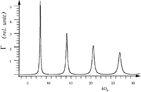
Figure 4: The magnetic field dependence for the attenuation rate of the longitudinal sound wave at $kr\gg 1$.

One can easily derive explicit expressions for $\Gamma$ at any $kr\eta$ making use of an example of a layered conductor whose electron spectrum has the form

$$\varepsilon(\boldsymbol{p})=\frac{p_{x}^{2}+p_{y}^{2}}{m}+\eta\frac{\hbar}{a}v_{0}\cos\left(\frac{ap_{z}}{\hbar}\right),\quad v_{0}=\frac{2\varepsilon_{\rm F}}{m},$$ (4.19)

and assume that the magnetic field is perpendicular to the layers [43]. In this case, at the lowest order in the small parameters $\gamma$ and $(kr)^{-1}$ the conductivity component is of the form

$$\sigma_{yy}=\frac{2Ne^{2}\tau}{\pi mkr_{0}}[1-J_{0}(kR\eta)\sin(2kr_{0})],$$ (4.20)

where $N$ is the charge carriers density, $r_{0}=v_{0}/\Omega$, $\Omega=eH/mc$, $R=2hc/eHa$ and $J_{0}$ is the Bessel function.

For $kR\eta\gg 1$, the Fermi surface corrugation is essential, and the acoustic absorption is similar to that in an ordinary (nearly isotropic) metal:

$$\Gamma=\frac{Nm\omega n_{0}}{4\pi\rho s^{2}}\Omega\tau\left[1+\left(\frac{2}{\pi kR\eta}\right)^{1/2}\cos\left(kR\eta-\frac{\pi}{4}\right)\sin(2kr_{0})\right]_{k=\omega/s}$$ (4.21)

for $kR\eta\ll 1$, peculiar properties of a quasi-two-dimensional conductor are manifested clearly, and $\Gamma$ is described by the expression

$$\Gamma = \frac{Nm\omega v_{0}}{4\pi\rho s^{2}}\Omega\tau$$ (4.22)

$$\times \mbox{Re}\,\Biggl{[}(\pi\gamma)^{2}+\frac{(kR\eta)^{2}}{2}+i\mu[1+\sin(2kr_{0})]$$

$$\times \biggl{(}1-\sin(2kr_{0})+\frac{(\pi\gamma)^{2}}{2}+\frac{(kR\eta)^{2}}{2}$$

$$+ \frac{1}{2}\left(\frac{3}{4kr_{0}}\right)^{2}+i\mu\biggr{)}^{-1}\Biggr{]}_{k=\omega/s},$$

where

$$\mu=\frac{\pi v_{0}c^{2}\omega}{2s^{3}\omega^{2}_{0}\Omega\tau}$$

and $\omega_{0}$ is the plasma frequency. If it is comparable to that of ordinary metals ($10^{15}$–$10^{16}$ s^-1), the parameter $\mu$ in the range of ultrasonic frequencies is fairly small, and the function $\Gamma(1/H)$ has giant resonant oscillations. This shape of $\Gamma(1/H)$ is usual for any electron spectrum described by Equation (1.1).

It should be noted that the resonance attenuation of acoustic waves in ordinary metals in a magnetic field is observed only if the charge carriers drift along the direction of the wave vector [35].

In the case of transverse acoustic wave polarization, $\boldsymbol{u}=(0,u_{y},u_{z})$, the external magnetic field $\boldsymbol{H}=(0,H_{y},H_{z})$ is contained only in expressions for acousto-electric coefficients, hence

$$E_{\alpha}=\frac{m\omega^{2}}{e}u_{\alpha}+\xi j_{\alpha}.$$

Having excluded $\tilde{E}_{\alpha}$ using Equation (4.8), we obtain

$$j_{y}(1-\xi\tilde{\sigma}_{yy})-j_{z}\xi\tilde{\sigma}_{yz} = \left(k\omega\tilde{a}_{yy}+\frac{m\omega^{2}}{e}\tilde{\sigma}_{yy}\right)u_{y}$$

$$+ \left(k\omega\tilde{a}_{yz}+\frac{m\omega^{2}}{e}\tilde{\sigma}_{yz}\right)u_{z},$$

$$-j_{y}\xi\tilde{\sigma}_{zy}+j_{z}(1-\xi\tilde{\sigma}_{zz}) = \left(k\omega\tilde{a}_{zy}+\frac{m\omega^{2}}{e}\tilde{\sigma}_{zy}\right)u_{y}$$ (4.23)

$$+ \left(k\omega\tilde{a}_{zz}+\frac{m\omega^{2}}{e}\tilde{\sigma}_{zz}\right)u_{z}.$$

Taking a combination of these equations with the elasticity equations (4.3), we obtain the equation system, whose self-consistency condition

$$\left|{\scriptsize\begin{array}[]{cccc}1-\xi\tilde{\sigma}_{yy}\!\!\!\!&\!\!\!\!-\xi\tilde{\sigma}_{yz}\!\!\!\!&\!\!\!\!\chi_{yy}\!\!\!\!&\!\!\!\!\chi_{yz}\\ -\xi\tilde{\sigma}_{zy}\!\!\!\!&\!\!\!\!1-\xi\tilde{\sigma}_{zy}\!\!\!\!&\!\!\!\!\chi_{zy}\!\!\!\!&\!\!\!\!\chi_{zz}\\ (i\omega m/e)+ik\xi\tilde{b}_{yy}\!\!\!\!&\!\!\!\!ik\xi\tilde{b}_{yz}\!\!\!\!&\!\!\!\!(\omega^{2}-s^{2}_{y}k^{2})\rho+\phi_{yy}\!\!\!\!&\!\!\!\!\phi_{yz}\\ ik\xi\tilde{b}_{zy}\!\!\!\!&\!\!\!\!(i\omega m/e)+ik\xi\tilde{b}_{zz}\!\!\!\!&\!\!\!\!\phi_{zy}\!\!\!\!&\!\!\!\!(\omega^{2}-s^{2}_{z}k^{2})\rho+\phi_{zz}\end{array}}\right|=0$$ (4.24)

yields damping parameters of the acoustic wave and the co-moving electromagnetic wave. Here $s_{y}=(\lambda_{yzyx}/\rho)^{1/2}$ and $s_{z}=(\lambda_{zxzx}/\rho)^{1/2}$ are the velocities of $y$- and $z$-polarized sound, respectively;

$$\chi_{\alpha\beta} = -k\omega\tilde{a}_{\alpha\beta}-\frac{m\omega^{2}}{e}\tilde{\sigma}_{\alpha\beta},$$

$$\phi_{\alpha\beta} = ik\left[k\omega\tilde{c}_{\alpha\beta}+\frac{m\omega^{2}}{e}\tilde{b}_{\alpha\beta}\right],$$ (4.25)

and the components of the elastic tensor, $\lambda_{yxzx}$ and $\lambda_{zxyx}$, equal to zero if, for example, the $xy$ plane is a crystal symmetry plane [44]. Otherwise these components should be taken into account, but they do not essentially affect the result. This crystal symmetry is implied in Equation (1.1).

The pronounced anisotropy of the electron spectrum in layered conductors leads to different attenuation lengths of sound with polarizations perpendicular and parallel to the layers, in the limit of small $\eta$, the displacement of ions along the normal to the layers decays over a length $\eta^{-2}$ times larger than a wave with $y$-polarization. One can easily prove that expansions in powers of $\eta$ of the components of acousto-electronic tensors with one or two $z$ indices start with terms of second or higher order. Omitting in Equation (4.24) terms of the order higher than two with respect to $\eta$, we obtain

$$[(\omega^{2}-s_{y}^{2}k^{2})\rho+\phi_{yy}](1-\xi\tilde{\sigma}_{zz})\chi_{yy}\left[\frac{i\omega m}{e}+ik\xi\tilde{b}_{yy}\right] ?$$

$${}[(\omega^{2}-s_{z}^{2}k^{2})\rho+\phi_{zz}]\left[1-\xi\tilde{\sigma}_{zz}-\chi_{zz}\frac{i\omega m}{e}\right] = 0$$

Since Equation (4.26) is factored, acoustic waves with $y$- and $z$-polarization do not interfer in this approximation. By equating to zero the first miltiplicator in (4.26), we obtain the equation for $k=\omega/s_{y}+k_{2}$, from which follows

$$k_{2} = \frac{i}{2\rho s_{y}^{2}(1-\xi\tilde{\sigma}_{yy})}\biggl{[}\xi k\omega(\tilde{a}_{yy}\tilde{b}_{yy}-\tilde{c}_{yy}\tilde{\sigma}_{yy})$$ (4.27)

$$+ \frac{m\omega^{2}}{e}(\tilde{a}_{yy}+\tilde{b}_{yy})k\omega\tilde{c}_{yy}+\frac{m^{2}\omega^{3}}{ke^{2}}\tilde{\sigma}_{yy}\biggr{]}_{k=\omega/s_{y}}.$$

The denominator in this equation is similar to that in the equation for $k_{1}$, so the absorption of the $y$-polarized wave has the same resonances as the longitudinal wave.

The deviation of the other root of Equation (4.26) from $\omega/s$ is proportional to $\eta^{2}$ when $\eta\to 0$ and described by the expression

$$k_{3} = \frac{i}{2\rho s_{z}^{2}}\Biggl{[}\frac{m\omega^{2}}{e}\left(\frac{\tilde{a}_{zz}}{1-\xi\tilde{\sigma}_{zz}}+\tilde{b}_{zz}\right)+\left(\frac{m\omega^{2}}{e}\right)^{2}\frac{s_{z}\tilde{\sigma}_{zz}}{1-\xi\tilde{\sigma}_{zz}}$$ (4.28)

$$+ \frac{\omega^{2}}{s_{z}}\tilde{c}_{zz}\Biggr{]}_{k=\omega/s_{z}}.$$

The transparency of the layered conductor for the acoustic wave with the polarization parallel to the normal to the layers occurs only at selected values of a magnetic field when $\sin kD=-1$. If $\sin kD$ differs essentially from $-1$ the sound attenuation rate has the form [45]:

$$\Gamma=\frac{\omega\tau}{r}\eta^{2}\{1+\sin kD+kr\eta^{2}(1-\sin kD)\}.$$ (4.29)

At a higher magnetic field, when $kr\ll 1$, acousto-electronic coefficients appear to be very susceptible to the magnetic field orientation with respect to the layers [46]. If in the expression for $\Lambda_{zz}$ and $v_{z}$, i.e.

$$\Lambda_{xx}(\boldsymbol{p}) = \sum\limits_{n=1}^{\infty}\Lambda_{n}(p_{x},p_{y})\cos\frac{anp_{z}}{\hbar};$$ (4.30)

$$v_{z}(\boldsymbol{p}) = -\sum\limits_{n=1}^{\infty}n\varepsilon_{n}(p_{x},p_{y})\frac{a}{h}\sin\frac{anp_{z}}{\hbar}$$ (4.31)

the functions $\Lambda_{n}(p_{x},p_{y})$ and $\varepsilon_{n}(p_{x},p_{y})$ decrease rapidly with $n$, the asymptotic form of the acousto-electronic coefficients are essentially different at some angles $\theta$ between the magnetic field and the normal to the layers. These are the values $\theta=\theta_{\rm c}$ at which $\eta^{2}$ in the expansion in powers of $\eta$ equal zero. For $\tan\theta\gg 1$ these terms turn to zero repeatedly with a period $\Delta(\tan\theta)=2\pi\hbar/D_{\rm p}$, where $D_{\rm p}$ is the Fermi surface diameter along the $p_{y}$ axis. These oscillations are due to the Larmour precession of electrons in strongly elongated cross-sections of the Fermi surface which intersect a large number of cells in the reciprocal lattice, while the oscillation period is associated with a change of this number by unity.

In the case when the dispersion law is described by Equation (4.19), $\Gamma(\eta)$ is given by

$$\Gamma=\eta^{2}\frac{Nm\omega v_{0}}{4\pi\rho s^{2}}\frac{sl}{r^{2}\omega}\frac{J_{0}^{2}(\zeta)\sin\theta}{1+\alpha^{2}J_{0}^{2}(\zeta)},$$ (4.32)

where

$$\alpha=\eta^{2}\frac{s\omega_{0}^{2}\tau}{c^{2}\omega},\quad\zeta=\frac{av_{0}m}{h}\tan\theta.$$

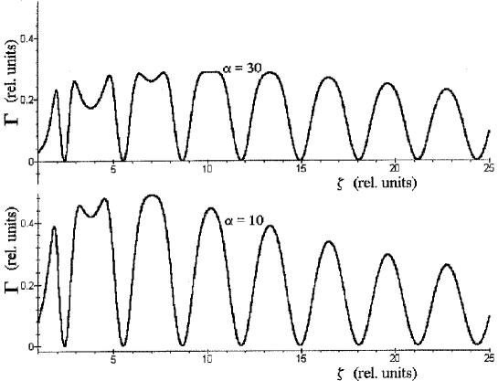
Figure 5: The angular dependence of the sound attenuation rate at $kr\ll 1$.

If the plasma frequency comparable with the value $\omega_{0}\sim 10^{15}$–$10^{16}$ s^-1 for a “good metal”, the parameter $\alpha$ is generally not small in spite of a small value of $\eta$. This complicates the form of the angular oscillations of $\Gamma$ (Fig. 5) [46].

One can easily find that the last term in expression (4.28) is a factor of $(v_{\rm F}/s_{z})^{2}$ larger than other term in brackets. If $\theta$ is different from $\theta_{\rm c}$, the following expression can be derived for $\Gamma=\mbox{Im}\,k_{3}$ for $kr\ll 1$ and $\omega\tau\ll 1$:

$$\Gamma=\frac{N\varepsilon_{\rm F}}{\rho s_{z}^{3}}\omega^{2}\tau\eta^{2}.$$ (4.33)

But at $\theta=\theta_{\rm c}$ the acoustic attenuation length $l_{\rm at}=1/\Gamma$ is considerably larger because $\Gamma$ takes the form:

$$\Gamma=\frac{N\varepsilon_{\rm F}}{\rho s_{z}^{3}}\omega^{2}\tau\eta^{2}\left[\eta^{2}+(kr)^{2}+\left(\frac{s_{z}}{v_{\rm F}}\right)^{2}f(\eta)\right].$$ (4.34)

The latter term in Equation (4.34) is due to the mismatch between the zeros of the functions $\tilde{a}_{zz}(\theta)/\eta^{2}$ and $\tilde{b}_{zz}(\theta)/\eta^{2}$, on one side, and $\tilde{c}_{zz}(\theta)/\eta^{2}$, on the other side, at $\eta\to 0$.

For an electron spectrum of the form (1.1), (4.30), (4.31) the acousto-electronic coefficients $a_{zz}$ and $b_{zz}$ tend to zero at $\eta\to 0$ faster than $\eta^{2}$, i.e. $f(\eta)$ also tends to zero at a small $\eta$. Strictly speaking, this is the main feature of the electron spectrum (1.1). For this reason we retain the parameters $\tilde{a}_{zz}$ and $\tilde{b}_{zz}$ in the final formulas for $k_{3}$, although this does not correspond to the actual accuracy of the formulas, given the electron spectrum described by Equation (1.1).

If $\eta$ is not infinitesimal, but satisfies the condition

$$\frac{\omega c}{\omega_{0}s_{z}}(\omega\tau)^{-1/2}\ll\eta\ll 1,$$ (4.35)

the term $\xi\tilde{\sigma}_{zz}$ in the denominator of Equation (4.28) cannot be omitted. For $kr\gg 1$ the damping rate of the sound with $z$-polarization may have resonances if

$$\frac{\omega c}{\omega_{0}s_{z}}(\omega\tau)^{-1/2}\ll\eta\ll(kr)^{-1}\ll 1.$$ (4.36)

The condition of the magnetoacoustic resonance in rather strict for tetrathiafulvalene salts, which have been extensively investigated recently. In these compounds the mean free path is $10^{-3}$–$10^{-2}$ cm, and resonances can be observed at acoustic frequencies of the order of $10^{9}$ s^-1. But the effect of field orientation on the sound absorption can be observed in such layered materials at acoustic frequencies of the order of $10^{8}$ s^-1 because for $kr\ll 1$ the ratio of the electron mean free path to the acoustic wavelength is not essential, and only the condition $r\ll l$, which is fulfilled in a field of 10–20 T, is obligatory.

The specific behaviour of damping of acoustic waves with different polarization can be used in filters transmitting waves of a definite polarization, and sound absorption may be a very accurate tool for studying electron spectra in layered conductors.

If an electron drifts along the sound wavevector (for instance, the sound wave propagates along the $y$-axis) the sound decrement reduces in $(kl\eta)^{2}$ times for $r/l\ll kr\eta\ll 1$ [47]. The solution of the kinetic equation in this case takes the form

$$\psi=\{\exp(\nu T+i\bar{\boldsymbol{k}}\bar{\boldsymbol{v}}T)-1\}^{-1}\int\limits_{t}^{t+T}\mbox{d}t^{\prime}\,g(t^{\prime})\exp\{i\boldsymbol{k}[\boldsymbol{r}(t^{\prime})-\boldsymbol{r}(t)]\},$$ (4.37)

where $g(t)=\Lambda_{ji}(t)k_{i}u_{j}+e\boldsymbol{v}(t)\tilde{E}$.

At $1\ll kl\eta\ll l/r$ in the expansion in the powers of $\nu T$ and

$$\bar{\boldsymbol{k}}\bar{\boldsymbol{v}}T=\int\limits_{0}^{T}\mbox{d}t\,\boldsymbol{kv}(t)$$

of the factor in front of the integral, the terms proportional to $\bar{\boldsymbol{k}}\bar{\boldsymbol{v}}T$ are the most essential. Finally, in the case when the charge carriers drift along $\boldsymbol{k}$ with the velocity $\bar{v}_{y}=\bar{v}_{z}\tan\theta\cong\eta v\tan\theta$, in the expression for the rate of sound attenuation $\nu T$ should be replaced by $kr\eta\tan\theta$. If $kr\eta\tan\theta\gg 1$, i.e. during the free path time an electron is capable of drifting along the sound wavevector at distance which exceeds significantly the sound wavelength; the magnetoacoustic resonance predicted and studied theoretically by Kaner, Privorotsky and one of the authors of this paper [35] takes place. The resonance occurs at $\bar{\boldsymbol{k}}\bar{\boldsymbol{v}}T=2\pi n$ and in contrast to the case of an ordinary metal the amplitude of the resonant oscillations is determined by the parameter $kr\eta$ rather than by $kr$.

The formulas given above are valid when $\cos\theta\gg cD_{\rm p}/eHl$. If $\theta$ is close to $\pi/2$, i.e. $\cos\theta$ is so small that an electron has no time to make a total rotation along the orbit in a magnetic field, then the components of the tensors $\tilde{\sigma}_{yy}$ and $\tilde{\sigma}_{zz}$ are close to their values in the absence of a magnetic field. This results from the fact that in the quasi-two-dimensional conductor only the projection $H_{z}$ affects the charge carriers dynamics, and at $\eta\ll 1$ the component $H_{y}$ manifests itself only in small corrections in the parameter $\eta$.

At $\theta=\pi/2$ the dependence of the sound damping decrement on the magnetic field magnitude is present only in the terms that vanish when $\eta\to 0$, and the magnetoacoustic effects are pronounced in the case of the shear wave with the ionic displacement along a normal to the layers only. In the range of a sufficiently strong magnetic field ($kr\ll 1$) the attenuation rate for the wave with such polarization depends essentially on the magnitude of a magnetic field and its orientation with respect to the layers, and in the $\theta$-dependence of $\Gamma$ sharp peaks and dips appear. At $\tan\theta\gg 1$ they repeat periodically with the period $\Delta(\tan\theta)=2\pi\hbar/D_{\rm p}$. The concrete form of the $\theta$-dependence of $\Gamma$ is analogous to the angular dependence of the electromagnetic impedance for $kr\ll 1$.

When the acoustic waves propagate along the normal to the layers, the Maxwell equations have the form

$$\{1-\xi\tilde{\sigma}_{xx}(k)\}\tilde{E}_{x}-\xi\tilde{\sigma}_{xy}(k)\tilde{E}_{y} = \xi\tilde{a}_{xj}(k)u_{j}-(u_{y}H_{z}-u_{z}H_{y})\frac{i\omega}{c}$$

$$- \frac{m\omega^{2}u_{x}}{e};$$

$$-\xi\tilde{\sigma}_{yx}(k)\tilde{E}_{x}\{1-\xi\tilde{\sigma}_{yy}(k)\}\tilde{E}_{y} = \xi\tilde{a}_{yj}(k)u_{j}+u_{x}H_{z}\frac{i\omega}{c}$$ (4.38)

$$- \frac{m\omega^{2}u_{y}}{e}.$$

It is easy to see that the electric field and the components of the matrix $\tilde{\sigma}_{\alpha\beta}$ do not disappear when $\eta\to 0$ and, consequently, the induction mechanism of the sound waves attenuation is more significant. The drift of conduction electrons along the $z$-axis does not take place only for the magnetic field orientation in the layers-plane. If $\theta$ is not equal to $\pi/2$, at $kr\eta\ll 1$ the displacement of charge carriers along the wavevector for the period of motion in a magnetic field is much less than the sound wavelength. The acousto-electronic coefficients are of the same order of magnitude as the analogous values for the case of weak spatial dispersion being reduced in $kl\eta$ times, if $kl\eta\gg 1$.

The dependence of $\Gamma$ on $H$ occurs only in the range of magnetic fields when $kr\eta\gg 1$. At $\tan\theta\ll leH/cD_{\rm p}$ an ordinary magnetoacoustic resonance takes place and this is connected with the charge carriers drift along the sound wavevector. At $\theta=\pi/2$ electrons drift in the $xy$-plane only, that is the direction orthogonal to the wavevector. In this case the sound attenuation rate oscillates with $1/H$ which is analogous to the Pippard oscillations in metals

$$\Gamma(H)=\frac{\eta\omega\tau}{r}\left\{1-(kr\eta)^{-1/2}\beta\sin\left(\frac{kc\Delta D_{{\rm p}x}}{2eH}+\frac{\pi}{4}\right)\right\}.$$ (4.39)

Measurements of the period of these oscillations

$$\Delta\left(\frac{1}{H}\right)=\frac{4\pi e}{kcD_{{\rm p}x}},$$ (4.40)

enable the corrugation of the Fermi surface to be evaluated. Here $D_{{\rm p}x}$ is the difference between the maximum and minimum diameters along the axis $p_{x}$ at $p_{y}=0$. The condition $kr\eta\gg 1$ is very strict and can be satisfied in the range of a magnetic field where $r\ll l$ only for $\eta\geq 1/10$. Therefore, there are no grounds to expect that the clear dependence of $\Gamma$ on the magnitude and orientation of a magnetic field can be observed in the layered conductors.

4.2 Fermi-Liquid Effects

Charged elementary excitations in conductors form a Fermi liquid, and their energy spectrum is determined by the distribution function for quasiparticles. As a result, the response of the electron system in solids to an external perturbation depends to a considerable extent on the correlation function describing the electron–electron interaction [48, 49]. Usually, the inclusion of the Fermi-liquid interaction of charge carriers leads to a renormalization of kinetic coefficients calculated on the assumption that conduction electrons form a Fermi gas. In some cases, however, the Fermi-liquid interaction approach leads to specific effects such as spin waves in nonmagnetic metals [50] and “softening” of metals in a strong magnetic field [51]. As a rule, in stationary fields Fermi-liquid effects results only in the renormalization of the charge carriers energy within the gas-approximation. For this reason, the analysis of the galvanomagnetic phenomena, when the charge carriers are assumed to form a Fermi-gas with an arbitrary electron energy spectrum, is equivalent to the consideration of the problem in the Fermi-liquid theory.

We consider the propagation of acoustic waves and co-moving electromagnetic waves with reference to the electron–electron interaction [52–54]. Charge carriers are supposed to form, not a Fermi-gas but a Fermi-liquid in which the correlation effects are essential.

Now the energy of charge carriers is a function of the density of elementary excitations. If the temperature is not too low, smearing of the equilibrium Fermi distribution function for charge carriers significantly exceeds the spacing between energy levels quantized by a magnetic field. In this case the energy of elementary excitations carrying a charge in the quasiclassical approximation has the form

$$\varepsilon=\varepsilon_{0}(\boldsymbol{p})+\lambda_{ij}(\boldsymbol{p})u_{ij}+\Psi(\boldsymbol{p},\boldsymbol{r},t),$$ (4.41)

where $\varepsilon_{0}(\boldsymbol{p})$ is the charge carriers energy in undeformed crystal in the gas approximation; the second term takes into consideration the renormalization caused by the deformation; and the function

$$\Psi(\boldsymbol{p},\boldsymbol{r},t)=\int\Phi(\boldsymbol{p},\boldsymbol{p}^{\prime})\delta f(\boldsymbol{p}^{\prime},\boldsymbol{r},t)\frac{2\mbox{d}^{3}p^{\prime}}{(2\pi\hbar)^{3}}$$ (4.42)

accounts for the correlation effects associated with the electron–electron interaction.

Here $\delta f=f(\boldsymbol{p},\boldsymbol{r},t)-f_{0}\{\varepsilon_{0}(\boldsymbol{p})\}$ is the nonequilibrium correction to the Fermi distribution function $f_{0}\{\varepsilon_{0}(\boldsymbol{p})\}$ for charge carriers in the undeformed conductor.

The Landau correlation function $\Phi(\boldsymbol{p},\boldsymbol{p}^{\prime})$ can be expanded in the complete set of orthonormal functions $\phi_{n}(\boldsymbol{p})$:

$$\Phi(\boldsymbol{p},\boldsymbol{p}^{\prime}) = \sum\limits_{n=0}^{\infty}\Phi_{n}\phi_{n}(\boldsymbol{p})\phi_{n}(\boldsymbol{p}^{\prime});$$ (4.43)

$$-\int\phi_{n}(\boldsymbol{p})\phi_{m}(\boldsymbol{p})\frac{\partial f_{0}(\varepsilon_{0})}{\partial\varepsilon_{0}}\frac{2\mbox{d}^{3}p}{(2\pi\hbar)^{3}} = \langle\phi_{n}(\boldsymbol{p})\phi_{m}(\boldsymbol{p})\rangle$$ (4.44)

$$= \delta_{nm},$$

and the nonequilibrium correction $\delta f(\boldsymbol{p},\boldsymbol{r},t)$ should be found by means of the solution for the kinetic equation

$$\frac{\partial f}{\partial t}+\frac{\partial f}{\partial\boldsymbol{r}}\frac{\mbox{d}\boldsymbol{r}}{\mbox{d}t}+\frac{\partial f}{\partial\boldsymbol{p}}\frac{\mbox{d}\boldsymbol{p}}{\mbox{d}t}=W_{\rm col}\{f\}.$$ (4.45)

The collision integral $W_{\rm col}\{f\}$ disappears being applied to the Fermi function $f_{0}(\varepsilon)$ depending on the charge carriers energy with regard to the correlation effects. Below we shall consider the collision integral in the $\tau$-approximation, i.e.

$$W_{\rm col}\{f\}=\frac{f_{0}(\varepsilon)-f}{\tau}=\frac{\Psi}{\tau}\frac{\partial f_{0}(\varepsilon)}{\partial\varepsilon}.$$ (4.46)

The equation of charge carriers motion in this case is of the form

$$\frac{\mbox{d}\boldsymbol{p}}{\mbox{d}t}=e\boldsymbol{E}+\frac{e}{c}\frac{\partial\varepsilon}{\partial(\boldsymbol{p}\times\boldsymbol{H})}-\frac{\partial\varepsilon}{\partial\boldsymbol{r}},$$ (4.47)

where the last tern accounts not only for the force of the deformation but also for the Fermi-liquid interaction of charge carriers.

In the linear approximation in a weak perturbation of charge carriers the kinetic equation (4.45) takes the form

$$\left\{\frac{\partial\Psi}{\partial t}+e\boldsymbol{Ev}+\Lambda_{ij}\frac{\partial u_{ij}}{\partial t}-\frac{\partial\psi}{\partial t}-\boldsymbol{v}\frac{\partial\psi}{\partial\boldsymbol{r}}-\frac{\partial\psi}{\partial t_{\rm H}}\right\} \times$$

$$\frac{\partial f_{0}(\varepsilon_{0})}{\partial\varepsilon_{0}} = \frac{\psi}{\tau}\frac{\partial f_{0}(\varepsilon_{0})}{\partial\varepsilon_{0}}$$

or

$$\frac{\partial\psi}{\partial t}+\boldsymbol{v}\frac{\partial\psi}{\partial\boldsymbol{r}}+\frac{\partial\psi}{\partial t_{\rm H}}+\frac{\psi}{\tau}=\frac{\partial\Psi}{\partial t}+e\tilde{\boldsymbol{E}}Bv+\Lambda_{ij}\frac{\partial u_{ij}}{\partial t},$$ (4.49)

where

$$\boldsymbol{v} = \frac{\partial\varepsilon_{0}}{\partial\boldsymbol{p}},$$

$$\frac{\partial\psi}{\partial t_{\rm H}} = \frac{e}{c}\frac{\partial\varepsilon_{0}}{\partial(\boldsymbol{p}\times\boldsymbol{H})}$$ (4.50)

the function $\Psi(\boldsymbol{p},x)$ is found with the help of the solution for the following integral equation:

$$\Psi(\boldsymbol{p},x,t) = \int\Psi(\boldsymbol{p},\boldsymbol{p}^{\prime})\{\Psi(\boldsymbol{p}^{\prime},x,t)-\psi(\boldsymbol{p}^{\prime},x,t)\}$$ (4.51)

$$\times \frac{\partial f_{0}(\varepsilon_{0}^{\prime})}{\partial\varepsilon_{0}^{\prime}}\frac{2\mbox{d}^{3}p^{\prime}}{(2\pi\hbar)3},$$

where $\varepsilon_{0}^{\prime}=\varepsilon_{0}(\boldsymbol{p}^{\prime})$.

Using the Fourier representation

$$\Psi(\boldsymbol{p},\boldsymbol{r})=\sum\limits_{n=0}^{\infty}\int\mbox{d}k\,\Psi_{n}(k)\phi_{n}(\boldsymbol{p})\exp\{i\boldsymbol{kr}\},$$ (4.52)

we obtain the following system of the algebraic equations for the Fourier transforms $\Psi_{n}(k)$:

$$\displaystyle\Psi_{n}(k)\{1+\Phi_{n}^{-1}\}+i\omega\langle\phi_{n}(\boldsymbol{p})\hat{R}\sum\limits_{m}\phi_{m}(\boldsymbol{p})\rangle\Psi_{m}(k)=$$

$$\displaystyle-ik_{j}u_{i}(k)\langle\phi_{n}(\boldsymbol{p})\Lambda_{ij}(\boldsymbol{p})\rangle+\langle\phi_{n}(\boldsymbol{p})\hat{R}[e\boldsymbol{v}\tilde{\boldsymbol{E}}(k)-k_{j}\omega\Lambda_{ij}(\boldsymbol{p})u_{i}(k)]\rangle,$$

where

$$\hat{R}g=\int\limits_{-\infty}^{t}\mbox{d}t^{\prime}\,g(t)\exp\{i\boldsymbol{k}[\boldsymbol{r}(t^{\prime})-\boldsymbol{r}(t)]+\nu(t^{\prime}-t)\}.$$ (4.54)

The value of $\omega\tau$ is smaller than unity even in pure conductors at low temperatures in a wide acoustic frequency range, and the integral term in Equation (4.53) can he taken into account in the perturbation theory. In the asymptotic approximation in the small parameter $\omega\tau$, the Fourier transform of the kinetic equation solution $\psi(k)$ is of the form

$$\psi(k) = \hat{R}\{e\tilde{E}_{j}(k)v_{j}+k_{i}\omega\Lambda_{ji}u_{j}(k)\}-i\omega\hat{R}\sum\limits_{n}\Phi_{n}(1+\Phi_{n})^{-1}$$ (4.55)

$$\times [\langle\phi_{n}\hat{R}e\tilde{E}_{j}v_{j}\rangle-ik_{i}u_{j}\langle\phi_{n}\Lambda_{ji}\rangle+\omega\langle\phi_{n}\Lambda_{ji}\rangle k_{i}u_{j}]\phi_{n}$$

and the acousto-electronic coefficients can be found easily. In the case, when $\boldsymbol{k}=(k,0,0)$ and displacement of ions is in the $xy$-plane, they are given by

$$\sigma_{ij}(k) = \langle e^{2}v_{i}\hat{R}v_{j}\rangle$$ (4.56)

$$- i\omega e^{2}\sum\limits_{n=1}^{\infty}\Phi_{n}(1+\Phi_{n})^{-1}\langle v_{i}\hat{R}\phi_{n}\rangle\langle\phi_{n}\hat{R}v_{j}\rangle;$$

$$a_{ij}(k) = \langle ev_{i}\hat{R}\Lambda_{jm}\rangle-\sum\limits_{n=1}^{\infty}\Phi_{n}(1+\Phi_{n})^{-1}\langle ev_{i}\hat{R}\phi_{n}\rangle$$ (4.57)

$$\times \left\{\langle\phi_{n}\lambda_{jm}\rangle\frac{k_{m}}{k}+i\omega\langle\phi_{n}\hat{R}\Lambda_{jm}\rangle\right\};$$

$$b_{ij}(k) = \langle e\Lambda_{i}\hat{R}v_{j}\rangle$$ (4.58)

$$- i\omega e\sum\limits_{n=1}^{\infty}\Phi_{n}(1+\Phi_{n})^{-1}\langle\Lambda_{ix}\hat{R}\phi_{n}\rangle\langle\phi_{n}\hat{R}v_{j}\rangle;$$

$$c_{ij}(k) = \langle e\Lambda_{ix}\hat{R}\Lambda_{jx}\rangle-\sum\limits_{n=1}^{\infty}\Phi_{n}(1+\Phi_{n})^{-1}$$ (4.59)

$$\times \langle e\Lambda_{ix}\hat{R}\phi_{n}\rangle\{\langle\phi_{n}\Lambda_{jx}\rangle+i\omega\langle\phi_{n}\hat{R}\Lambda_{jx}\rangle\}.$$

Using Equations (4.56)–(4.59) we can easily determine the rate of absorption for the acoustic wave. For brevity of computations only, we assume that $\phi_{1}(-\boldsymbol{p})=\phi_{1}(\boldsymbol{p})$ and $\phi_{2}(-\boldsymbol{p})=-\phi_{2}(\boldsymbol{p})$, while $\phi_{n}$ with $n>2$ are equal to zero. Taking into account that $\varepsilon(-\boldsymbol{p})=\varepsilon(\boldsymbol{p})$, at $\eta\ll kr\eta\ll 1$ we obtain for $\sigma_{yy}$ the following expression:

$$\sigma_{yy}^{\rm liquid}=\sigma_{yy}^{\rm gas}(1-L),$$ (4.60)

where

$$L=\frac{i\omega\Omega\langle 1\rangle}{\pi\nu kv}\left\{\frac{\Phi_{1}}{1+\Phi_{1}}\phi_{1}^{2}(1+\sin kD)+\frac{\Phi_{2}}{1+\Phi_{2}}\phi_{2}^{2}(1-\sin kD)\right\},$$ (4.61)

and $\phi_{1}$, $\phi_{2}$ and $v$ are the values of the functions $\phi_{i}(t)$ and the velocity modulus in the point where $\boldsymbol{kv}=\omega$.

At $kr\ll 1$ the angular dependence of neither the electromagnetic impedance nor the sound attenuation rate undergo substantial changes due to the allowance for the Fermi-liquid interaction between charge carriers.

Naturally, the acoustic transparency and the sound attenuation rate of layered conductors with a quasi-two-dimensional electron energy spectrum depend on the intensity of the Fermi-liquid interaction between charge carriers. The inclusion of the Fermi-liquid interaction significantly affects the shape of the resonance curve but the period of oscillations of $\Gamma$ with $1/H$ and the positions of sharp peaks in the angular dependence $\Gamma(\theta)$ remain unchanged when Fermi-liquid effects are taken into account.

The magnitude of the Fermi-liquid interaction between charge carriers can be determined from measured electromagnetic and acoustic impedances either for different wave frequencies or at sufficiently low temperatures, when effects of the charge carriers energy quantization are manifested clearly.

5. POINT-CONTACT SPECTROSCOPY OF LAYERED
CONDUCTORS

5.1 Point-Contact Investigation of Electron Energy Spectrum

In 1965 Sharvin [55] studied the dynamics of conduction electrons by using a magnetic field for longitudinal focusing of carriers injected into a metal from a point contact. Figure 6 shows the schematic diagram of the circuit for longitudinal electron focusing, in which an uniform magnetic field $\boldsymbol{H}$ is directed along the line connecting two point contacts, viz., the emitter E and the collector C situated at the opposite surfaces of a thin plate. The longitudinal electron focusing was first observed by Sharvin and Fisher [56].

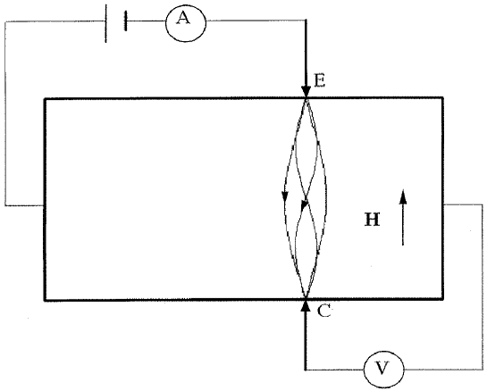
Figure 6: The schematic diagram of the circuit for observing longitudinal electron focusing.

Another possibility for observing focused electron beams in metals is associated with the geometry of the experiments in which the magnetic field $\boldsymbol{H}$ is directed at a right angle to the line connecting the contacts at the same surface of the sample (transverse electron focusing). This idea was proposed by Pippard [57] and first realized experimentally by Tsoi [58]. The diagram of a circuit for transverse electron focusing is shown in Fig. 7.

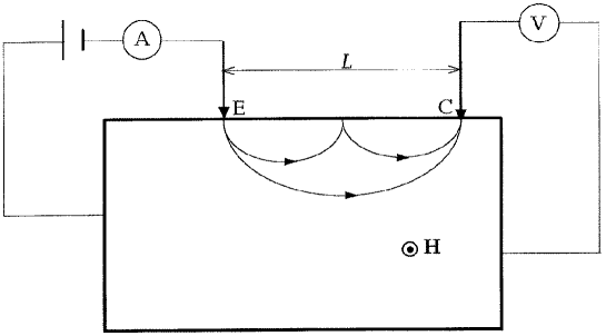
Figure 7: The schematic diagram of the circuit for observing transverse electron focusing.

It was noted even in first experimental [55, 58] and theoretical [59, 60] publications that electron focusing, a ballistic effect in its origin, is extremely sensitive to the energy-momentum relation for charge carriers, and the electron focusing signal might have extrema due to electrons belonging to open Fermi surface cross-sections [60]. A peculiar feature of the further analysis is the quasi-two-dimensional nature of the electron energy spectrum which is responsible for a significant difference in both the amplitude and the shape of electron focusing for the layered conductors and for metals with weakly anisotropic conducting properties [61]. This difference is associated with a small displacement of electrons in the direction perpendicular to the layers over the time of their motion from one point contact to another, and as a result, with the dependence of the electron focusing signal on the relation between the above displacement and point contact diameters.

Let us consider a standard experimental geometry for electron focusing observations, when the current point contact (emitter E) and the measuring point contact (collector C) are mounted either on the same surface or on the opposite surfaces of a plate. The quantity under investigation is the difference (measured by a voltmeter) in electrochemical potentials of the collector and a periphery point of the sample as a function of the magnitude and direction of the magnetic field $\boldsymbol{H}$.

In order to determine quantity $U$, measured with the aid of potential point contacts, let us consider a stationary nonequilibrium electron state described by the distribution function

$$f(\boldsymbol{p},\boldsymbol{r})=f_{0}(\varepsilon)-e\frac{\partial f_{0}}{\partial\varepsilon}(x_{\boldsymbol{p}}-\phi(\boldsymbol{r}))$$ (5.1)

which satisfies the Boltzman equation (2.2) supplemented by the boundary condition on the sample surface $\boldsymbol{R}\in\Sigma$

$$f(\tilde{\boldsymbol{p}},\boldsymbol{R})\!\!\! = \!\!\!f(\boldsymbol{p},\boldsymbol{R})$$ (5.2)

$$+ \!\!\!\int\mbox{d}^{3}\boldsymbol{p}^{\prime}\,\Theta(-v_{n}^{\prime})W(\boldsymbol{p},\boldsymbol{p}^{\prime})[f_{\boldsymbol{p}^{\prime}}(\boldsymbol{p}^{\prime},\boldsymbol{R})-f(\boldsymbol{p},\boldsymbol{R})]\Theta(\boldsymbol{R}\notin S_{i})$$

$$+ \!\!\!\sum\limits_{i}f^{(i)}(\boldsymbol{p},\boldsymbol{R})\Theta(\boldsymbol{R}\in S_{i}),$$

where $v_{n}=\boldsymbol{vn}$; $\boldsymbol{n}$ is the interior normal to the specimen boundary; $\Theta(x)$ is, as before, the Heaviside function, $\Theta(\boldsymbol{R}\in S_{i})$ is a unit function that differs from zero for values of $\boldsymbol{R}$ belonging to the plane $S_{i}$ of the $i$-th contact opening; $\Theta(\boldsymbol{R}\notin S_{i})=1-\Theta(\boldsymbol{R}\in S_{i})$; $f^{(i)}(\boldsymbol{p},\boldsymbol{R})$ is the electron-distribution function on the plane $S_{i}$. The electron monenta $\tilde{\boldsymbol{p}}$ and $\boldsymbol{p}$ are connected through the specular reflection conditions:

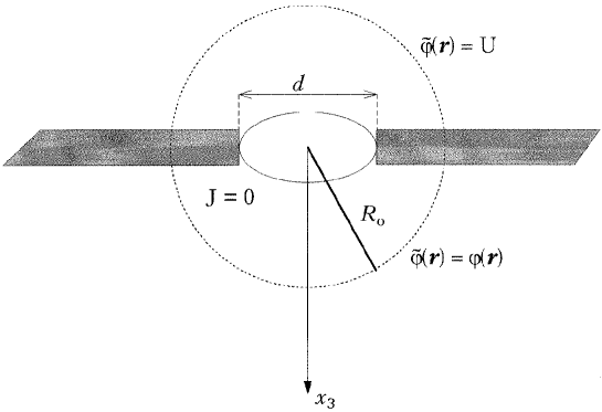
Figure 8: A model of the measuring contact (collector C) shaped as a circular orifice of a diameter $d$.

$$\varepsilon(\boldsymbol{p})=\varepsilon(\tilde{\boldsymbol{p}});\quad[\boldsymbol{pn}]=[\tilde{\boldsymbol{p}}\boldsymbol{n}].$$ (5.3)

The Equation (5.2) takes into account the surface scattering of electrons and the injection of charge carriers into the sample through the current and potential contacts. The kernel of the integral operator $W(\boldsymbol{p},\boldsymbol{p}^{\prime})$ (the surface scattering indicatrix) depends on the nature of the surface scattering (see [62–64]). The function $f^{(i)}(\boldsymbol{p},\boldsymbol{R})$ depends on the contact shape and the nature of its contamination, and must be found by solving a kinetic equation in the contact region. The condition (5.2) automatically ensures the current does not flow across the surface and potential contacts, and is conserved in the plane of the current orifice. The electric field $\boldsymbol{E}(\boldsymbol{r})=-\nabla\phi(\boldsymbol{r})$ in the sample is determined from the electroneutrality condition (3.15).

In the case of a bulk layered conductor and the current contacts of a large area which are placed at the opposite surfaces of the sample we can ignore the surface effects and not consider the boundary condition (5.2). It is well known [65], that at distances from the sample boundaries larger than the maximum mean free path of electrons $l$, an uniform electric field $\boldsymbol{E}(\boldsymbol{r})=\mbox{const}$ automatically satisfies the equation of electrical neutrality (3.15), and the relation between a current density $\boldsymbol{j}$ and an electric field $\boldsymbol{E}$ has an ordinary form (2.1).

Let a point contact C with an ideal voltmeter (of an infinite resistance) connected to it, be situated at the metal surface. The diameter $d$ of the contact is presumed to be much less than $l$. A transient current which appears at the initial moment will nullify as the potential far from the contact (at distances $|\boldsymbol{R}_{0}|\gg d$) in the bulk reaches a certain value $U$ (Fig. 8). We shall assume that the second potential contact is placed at the specimen periphery ($\boldsymbol{r}\to\infty$, $x>0$) where $f(\boldsymbol{p})=f_{0}(\varepsilon)$ and $\phi=0$. Then the potential difference, as measured by voltmeter, will be equal to $U$. The condition of the absence of the current $J$ through the measuring contact orifice can be written by representing the distribution function in the form

$$f(\boldsymbol{p},\boldsymbol{r}) = f_{0}(\varepsilon)-e\frac{\partial f_{0}}{\partial\varepsilon_{p}}\left\{\begin{array}[]{ll}\tilde{\chi}_{\boldsymbol{p}}(\boldsymbol{r})-\tilde{\phi}(\boldsymbol{r}),&v_{3}<0\\ U-\tilde{\phi}(\boldsymbol{r}),&v_{3}>0\end{array}\right.;$$ (5.6)

$$J = \frac{2e^{2}}{(2\pi h)^{3}}\int\limits_{S_{\rm c}}\mbox{d}^{2}\boldsymbol{r}\,\langle v_{3}(U-\tilde{\chi}_{\boldsymbol{p}}(\boldsymbol{r}))\Theta(v_{3})\rangle=0.$$ (5.7)

In this chapter the angle brackets indicate the integration over Fermi surface

$$\langle\ldots\rangle=-\int\mbox{d}^{3}\boldsymbol{p}\frac{\partial f_{0}}{\partial\varepsilon}\ldots\,,$$

$v_{3}$ is the velocity component perpendicular to the contact plane (Fig. 8); $\tilde{\chi}_{\boldsymbol{p}}$ and $\tilde{\phi}(\boldsymbol{r})$ represent the function $\chi_{\boldsymbol{p}}$ and the potential $\phi$ being perturbed by the measuring contact. The integration in Equation (5.5) is carried out over the area of the contact orifice, $S_{\rm c}=\pi d^{2}/4$. At distances $|\boldsymbol{R}_{0}|\gg d$ from the contact we have

$$\tilde{\chi}_{\boldsymbol{p}}\cong\left\{\begin{array}[]{ll}\chi_{p},&x_{3}>0\\ 0,x_{3}<0\end{array}\right.;\quad\tilde{\phi}(\boldsymbol{r})\cong\left\{\begin{array}[]{ll}\phi(\boldsymbol{r}),&x_{3}>0\\ U,x_{3}<0\end{array}\right..$$ (5.8)

These relations are valid under the condition $d\ll|\boldsymbol{R}_{0}|\ll L_{0}$, where $L_{0}$ is the characteristic spatial scale of variation of the function $\chi_{\boldsymbol{p}}$ far from the contact C. When $d$ tends to zero, from Equations (5.5) and (5.6) we obtain the following expression for the quantity $U$ [66]:

$$U=\frac{\langle v_{3}\chi_{\boldsymbol{p}}(\boldsymbol{L})\Theta(-v_{3})\rangle}{\langle v_{3}\Theta(-v_{3})\rangle},$$ (5.9)

where the vector $\boldsymbol{L}$ defines the position of the measuring contact at the surface.

The function $\chi_{\boldsymbol{p}}(\boldsymbol{r})$ in the solution (5.1) of the kinetic equation (2.2) in the approximation of the relaxation time $\tau$ can be presented in the form

$$\chi_{\boldsymbol{p}}(\boldsymbol{r}) = F(\boldsymbol{r}-\boldsymbol{r}(t))\exp\left(\frac{\lambda-t}{\tau}\right)$$ (5.10)

$$+ \int\limits_{\lambda}^{t}\mbox{d}t^{\prime}\,\phi(\boldsymbol{r}+\boldsymbol{r}(t^{\prime})-\boldsymbol{r}(t))\exp\left(\frac{t^{\prime}-t}{\tau}\right),$$

where $\lambda(\boldsymbol{r},\boldsymbol{p})\leq t$ is the instant of time when an electron is reflected from the specimen boundary at the point $\boldsymbol{R}$ given by equation

$$\int\limits_{\lambda}^{t}\mbox{d}t^{\prime}\,\boldsymbol{v}(t^{\prime})=\boldsymbol{r}(t)-\boldsymbol{r}(\lambda)=\boldsymbol{r}-\boldsymbol{R},$$ (5.11)

$F(\boldsymbol{r}-\boldsymbol{r}(t))$ is an arbitrary function of characteristics whose value is preserved along the trajectory of motion of charge carriers between two collisions with the surface. The condition (5.2) enables us to obtain an explicit expression for the function $F$. Representing the distribution function of electrons leaving the emitter in the form

$$f^{(E)}(\boldsymbol{p},\boldsymbol{r})=f_{0}(\varepsilon)-\frac{\partial f_{0}}{\partial\varepsilon}(\chi_{\boldsymbol{p}}^{*}-\phi(\boldsymbol{r})),$$

we can write the following expression for the value of the function $\chi_{\boldsymbol{p}}$ in the plane $S_{\rm c}$,of the collector orifice [67]:

$$\chi_{\boldsymbol{p}}(\boldsymbol{L})=\chi_{\boldsymbol{p}}^{*}\sum\limits_{n}q^{n-1}\Theta(\boldsymbol{L}-\Delta\boldsymbol{R}_{n}\in S_{\rm E})\left(\exp-\frac{\Delta T_{n}}{\tau}\right)+\Delta\chi_{\boldsymbol{p}}(\boldsymbol{R}).$$ (5.12)

where

$$q(\boldsymbol{p})=1-\int\mbox{d}^{3}\boldsymbol{p}^{\prime}\,\Theta(-v_{n}^{\prime})W(\boldsymbol{p},\boldsymbol{p}^{\prime})$$

is the specular reflection parameter.

Equation (5.10) contains the summations over the number $n$ of collisions with the surface of electrons injected from the emitter. The displacement of these electrons in the plane parallel to the boundary during the time $\Delta T_{n}$ of motion from contact to contact is $\Delta R_{n}$. The first term on the right-hand side of Equation (5,10) is the nonequilibrium component of the distribution function for electrons moving strictly along ballistic trajectories. This term determines the part of the signal on the measuring contact, which depends nonmonotonically on the magnetic field and contains singularities (extremes and kinks) known as electron focusing lines. The second term in Equation (5.10) results from electron scattering in the bulk as well as from scattering on the surface of the conductor ($\Delta\chi_{\boldsymbol{p}}\to 0$, if $\tau\to\infty$, $q=1$). This term is responsible for the emergence of background in the $U(H)$ signal which varies smoothly with $\boldsymbol{H}$. In this version, we will consider a more informative (from the experimental point of view) situation when $\Delta T_{n}\ll\tau$ and $1-q\ll 1$, therefore we shall not adduce the explicit form of the function $\chi_{\boldsymbol{p}}(R)$ whose contribution to the electron focusing signal $U(H)$ can be discounted when the above inequalities are satisfied. In the case of pure contacts, whose diameter $d$ is much less than $l$, and relatively weak magnetic field, considered below, the affect of the field on electron trajectories can be discounted over a distance of the order $d$. In this case the function $\chi_{\boldsymbol{p}}^{*}$ is independent of the coordinate and momentum and is equal to the voltage $V$ applied to the contact [68].

In the case when the separation $L$ between the point contacts is much greater than the contact diameter $d$, the asymptotic behaviour of the integral in Equation (5.7) is conditioned by the fact that only a small faction of charge carriers starting from the emitter can reach the collector. These are electrons that belong to a small region of the Fermi surface near the points $p=p_{0}(\boldsymbol{H},n)$ specified by equations:

$$\Delta\boldsymbol{R}_{n}(\boldsymbol{p}_{0})=\boldsymbol{L}.$$ (5.13)

The approximation of the step function $\Theta(\boldsymbol{R}\in S_{\rm E})$ by the function $\exp[-|\boldsymbol{R}|^{2}/(d/2)^{2}]$ for $d/L\to 0$ allows us to find the asymptotic value of the quantity $U$ by using the Laplace method. Retaining the main term in the asymptotic series, it is convenient to write the amplitude of the electron focusing signal in the form

$$U(H)=V\sum\limits_{n=n_{0}}^{N}\exp\left(-\frac{\Delta T_{n}(p_{0})}{\tau}\right)A(\boldsymbol{p}_{0}),$$ (5.14)

where $n_{0}(\boldsymbol{H})$, $N(\boldsymbol{H})$ are the minimum and maximum numbers of collisions with the boundary by which an electron can reach the collector for a given value of the magnetic field. $A(\boldsymbol{p}_{0})$ is the partial contribution to the electron focusing signal from the electrons having a momentum $\boldsymbol{p}_{0}(\boldsymbol{H},n)$, and getting from the current contact to the measuring one without scattering. The form of function $A$ is determined by the mutual orientation of the crystal surface, line $\boldsymbol{L}$ connecting the contacts, and the magnetic field vector $\boldsymbol{H}$.

We shall consider below the two main experimental geometries when the axes of the contacts are either parallel or orthogonal to the layers with a high electrical conductivity, in addition to the expression for the function $A(\boldsymbol{p}_{0})$ which is valid for an arbitrary form of the functions $\varepsilon_{0}$ and $\varepsilon_{1}$ characterizing the Fermi surface (1.1), we shall give the results of calculations based on a commonly used simple model (2.21). This model enables us to obtain the magnetic field dependence of $U$ in an explicit form.

1. The contacts are on the crystal boundary perpendicular to the layers with a high electrical conductivity. In this geometry, it is possible to observe the transverse electron focusing by a magnetic field applied parallel to the boundary (Fig. 9a). If the vector $\boldsymbol{H}=(0,0,H)$ is oriented at an angle $\theta$ to the plane of the layers, charge carriers perform a periodic motion over the surface. Their displacement along the boundary $\Delta\boldsymbol{R}$ during the time $\Delta T$ between two collisions with the boundary is the same for all segments of the trajectory:

$$\Delta\boldsymbol{R}_{n} = n\Delta\boldsymbol{R}=(\Delta y_{n},\Delta z_{n})=\frac{nc}{eH}\left(D_{x},\frac{\partial S_{\rm seg}}{\partial p_{z}}\right)=\boldsymbol{L};$$

$$\Delta T_{n} = \frac{nc}{eH}\frac{\partial S_{\rm seg}}{\partial\varepsilon_{p}},$$ (5.15)

where $n$ is the number of a collision with the boundary, $D_{x}(p_{y},p_{z})$ is the chord of the section of the Fermi surface $\varepsilon(\boldsymbol{p})=\varepsilon_{\rm F}$ cut by the plane $p_{z}=\mbox{const}$, which is parallel to the normal $\boldsymbol{n}=(1,0,0)$ to the boundary; $S_{\rm seg}$ is the area of the segment cut by the chord $D_{x}$ on this section; and $\boldsymbol{L}=(0,L_{y},L_{z})$.

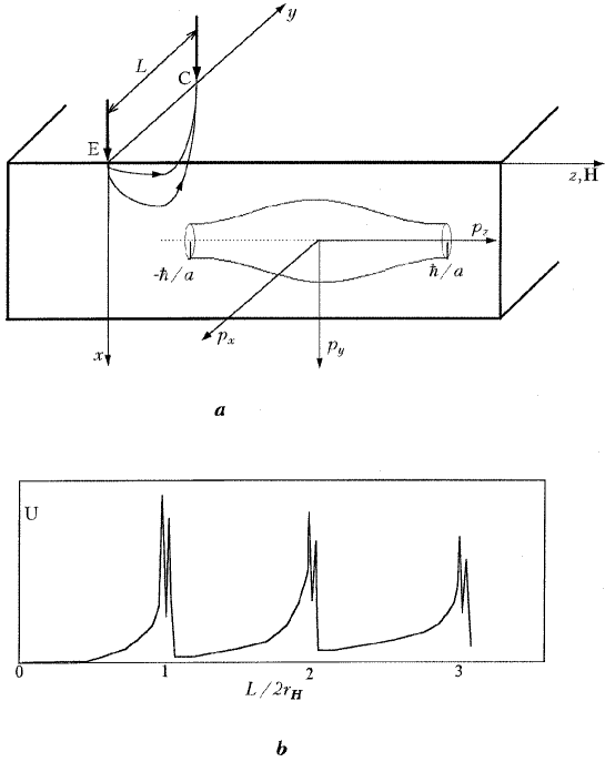
Figure 9: Experimental geometry (a) and the shape of the transverse ($\boldsymbol{L}\bot\boldsymbol{H}$) electron focusing peaks (b) in the case when the line $\boldsymbol{H}$ connecting the contacts on the same face of the crystal lies in the plane of the layers, and the magnetic field vector $\boldsymbol{H}$ is orthogonal to the layers.

The minimum number of the collisions $n_{0}$ with which an electron can reach the collector is connected with the maximum displacement $R_{m}=|\Delta R^{\rm max}|$ through the inequalities $L/R_{m}<n_{0}<L/R_{m}-1$, and the maximum number of the collisions $N$ tends to infinity and corresponds to charge carriers sliding over the crystal surface at very small angles.

The magnitude of the electron focusing amplitude is extremely sensitive to the relation between two small parameters $\mu=d/L$ and $\eta=\varepsilon_{1}/\varepsilon_{\rm F}$, that characterize the relative number of electrons participating in the formation of the signal and anisotropy of the energy spectrum, respectively. For $\mu\ll\eta$, only the charge carriers having momenta from the narrow strips on the Fermi surface ($\Delta p_{z}a/\hbar\simeq\mu$) can reach the collector ($a$ is the distance between the layers). In this case, the computation of the quantity $A$ in Equation (5.12) leads to the following results:

$$A(\boldsymbol{p}_{0})=\frac{D_{x}^{2}}{\langle v_{x}\Theta(-v_{x})\rangle}\left\{\begin{array}[]{ll}\displaystyle\frac{\pi}{4}\mu^{2}D^{-1},&D\neq 0\\[8.0pt] \displaystyle\frac{\sqrt{\pi}}{2}\Gamma\left(\frac{1}{4}\right)\mu^{3/2}Q^{-1};&D=0;\;Q\neq 0\end{array}\right.$$ (5.16)

where

$$D = \frac{\partial D_{x}}{\partial p_{y}}\frac{\partial^{2}S_{\rm seg}}{\partial p_{z}^{2}}+\left(\frac{\partial D_{x}}{\partial p_{z}}\right)^{2};$$

$$Q = \frac{\partial^{2}S_{\rm seg}}{\partial p_{z}^{2}}\left|D_{x}\frac{\partial^{2}D_{x}}{\partial p_{y}^{2}}\right|^{1/2}.$$

The peaks of the electron focusing signal correspond to the values of the field $H_{n}$ satisfying the condition (5.11) for which $D=0$.

If the large-diameter contacts satisfy the condition $1\gg\mu\gg\eta$ and the angle $\theta$ between the vector $\boldsymbol{H}$ and the Fermi surface cylinder axis is less than $\eta$, the drift $\Delta z_{n}$ along the $\boldsymbol{H}$-direction is smaller than the contact diameter $d$ for all electrons leaving the emitter. In other words, electrons with any value of the component $p_{z}$ can get from contact to contact. An increase in the number of electrons hitting the collector results in a stronger signal as compared to the situation when $\mu\ll\eta$. Assuming that the Fermi surface is cylindrical ($\varepsilon(\boldsymbol{p})=\varepsilon_{0}(p_{x},p_{y})$) in the main approximation in the parameter $\eta/\mu\ll 1$, we obtain the following expression for the function $A$:

$$A=\frac{D_{x}^{2}}{\langle v_{x}\Theta(-v_{x})\rangle}\left\{\begin{array}[]{ll}\displaystyle\sqrt{\pi}\mu\left|\frac{\partial D_{x}}{\partial p_{y0}}\right|^{-1},&\displaystyle\frac{\partial D_{x}}{\partial p_{y0}}\neq 0\\[8.0pt] \displaystyle\frac{\Gamma(1/4)}{2^{1/4}}\mu^{1/2}\left|D_{x}\frac{\partial^{2}D_{x}}{\partial p^{2}_{y0}}\right|^{-1/2},&\displaystyle\frac{\partial D_{x}}{\partial p_{y0}}=0\end{array}\right.$$ (5.17)

For $\boldsymbol{H}\bot\boldsymbol{L}$ (Fig. 9a), the electron focusing signal has peaks for those values of a magnetic field $H=H_{n}$ at which electrons, reaching the collector, have the maximum displacement along the surface and correspond to the extremal Fermi surface diameter ($D_{x}^{\rm ext}=D_{x}(p_{0e})$) [58–60]. However, separate observation of transverse electron focusing peaks associated with charge carriers belonging to different extremal cross sections of Fermi surface is possible only for contacts with a small diameter ($\mu\ll\eta$).

For a quadratic and isotropic energy-momentum relation for electrons in the layers (2.21) and for $\boldsymbol{H}\bot\boldsymbol{L}\bot p_{z}$ Equation (5.14) and (5.15) take the simple form

$$\mu\ll\eta$$

$$A = \frac{p_{\rm F}h}{m\varepsilon_{1}a}\left\{\begin{array}[]{ll}\displaystyle\mu^{2}\frac{\xi_{n}^{3}}{\arcsin(\xi_{n})\sqrt{1-\xi_{n}^{2}}},&\xi_{n}<1\\[8.0pt] \displaystyle\Gamma\left(\frac{1}{4}\right)\pi^{3/2}\mu^{3/2},&\xi_{n}=1\end{array}\right.$$ (5.20)

$$\mu\gg\eta$$

$$A = \left\{\begin{array}[]{ll}\displaystyle\frac{\sqrt{\pi}}{4}\mu\frac{\xi_{n}^{3}}{\sqrt{1-\xi_{n}^{2}}},&\xi_{n}<1\\[8.0pt] \displaystyle\Gamma\left(\frac{1}{4}\right)2^{9/2}\mu^{1/2},&\xi_{n}=1\end{array}\right.$$ (5.23)

where $n\geq n_{0}$; $\xi_{n_{0}}<1$, and $\xi_{n_{0}-1}>1$. The quantity $\xi_{n}$ in Equation (5.16) has the two values $\xi_{n}=L/2nr_{\rm H}(1\pm\eta)$ ($r_{\rm H}=cp_{\rm F}/eH$; $p_{\rm F}=\sqrt{2m\varepsilon_{\rm F}}$) for the same value of $n$, which correspond to the contributions from electrons belonging to the maximum and minimum Fermi surface cross-sections. We must put $\xi_{n}=L/2nr_{\rm H}$ in Equation (5.17) which is valid to within the terms proportional to $\eta/\mu\ll 1$.

The period of motion along the trajectory is a multiple valued function of $\xi_{n}$ ($\Delta T^{(1)}=(T_{\rm H}/\pi)\arcsin\xi_{n}$; $\Delta T^{(2)}=T_{\rm H}-\Delta T^{(1)}$; $T_{\rm H}=2\pi mc/eH$), since the same displacement over the surface corresponds to the two possible electron orbits with the height of segment $\Delta x^{(1,2)}=r_{\rm H}(1\pm\sqrt{1-\xi_{n}^{2}})$.

Figure 9b is plotted as a result of numerical calculations based on the Equations (5.12) and (5.16) and shows the $U(H)$ dependence for $\mu\ll\eta$. The split structure of the electron focusing peaks is due to a small difference between the extremal diameters of the cross-sections cut by $p_{z}=0$ and $p_{z}=\pm\hbar/a$.

The angle $\theta$ between the vector $\boldsymbol{H}$ and Fermi surface cylinder axis significantly affects the form of electron trajectories. As the value $\theta$ increases, the orbits become elongated along the normal to the sample boundary and acquire additional indentations associated with Fermi surface corrugation (see Fig. 2b). For certain magnetic field orientations, electron trajectories acquire saddle points (halt points), and the period of motion tends logarithmically to infinity (Equation (2.18)). With increasing $\theta$, the electron drift along the magnetic field is enhanced due to an increase in the period of motion along the trajectory as well as an increase in possible values of the electron velocity components along the vector $\boldsymbol{H}$ [69].

In accordance with the evolution of electron orbits described above, the rotation of the line connecting the contacts in the plane of the surface leads to a nonmonotonic dependence of the electron focusing signal amplitude on the angle $\theta$ [60] and to the emergence of additional electron focusing peaks associated with the emergence of new extremal diameters on the Fermi surface cross section satisfying Equation (5.11).

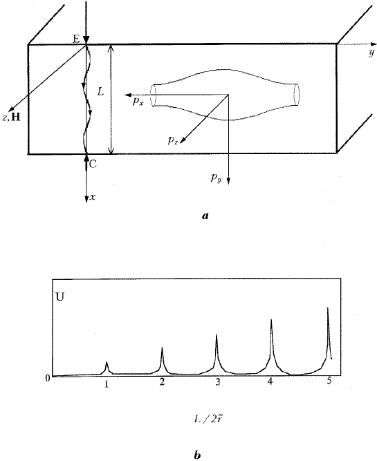
Figure 10: Experimental geometry (a) and the shape of the transverse ($\boldsymbol{L}\bot\boldsymbol{H}$) electron focusing peaks (b) in the case when the line $\boldsymbol{L}$ connects the contacts at opposite faces of a thin plate, and the magnetic field vector $\boldsymbol{H}$ lies in the plane of the layers.

In the limiting case when the vector $\boldsymbol{H}$ lies in the plane of the layers ($\theta=\pi/2$), charge carriers belonging to open Fermi surface cross sections move along periodic trajectories into the bulk of the sample, which allows the observation of the effect analogous to the longitudinal electron focusing with the help of the point contact located on the second surface of thin plate with the thickness $L<l$ (Fig. 10a). If both of the point contacts are on the $x$-axis, the electron from the emitter can reach the collector only if its displacement in the direction orthogonal to this axis over the time $\Delta T$ of motion from one surface of the plate to another is less then the contact diameter $d$. For $d\to 0$ we have the conditions:

$$\Delta\boldsymbol{R} = \left(\frac{c}{eH}(p_{x0}(\lambda+\Delta T),v_{z0}\Delta T)\right)=0,$$

$$\Delta x = \frac{c}{eH}(p_{y0}(\lambda+\Delta T)-p_{y0}(\lambda))=L,$$ (5.24)

where $\lambda$ characterizes the position of an electron on the Fermi surface at the moment of its “start” from the emitter. When the condition $2\pi\hbar ck/eHa=L$ ($k=1,2,\ldots$) is satisfied, the time $\Delta T=L/\bar{v}_{y}$ is multiple of the period of motion $T_{\rm op}$. In this case all the electrons have zero displacement along the $y$-axis, and the amplitude of the electron focusing signal attains its maximum value. For $\boldsymbol{L}\bot p_{z}\bot\boldsymbol{H}$, only the electrons that do not interact with the sample surface can get from contact to contact along the ballistic trajectory, and we must put $n_{0}=N=1$ in Equation (5.12). The partial contribution to the amplitude $A(\boldsymbol{p})$ is associated with electrons for which the focusing conditions (5.18) are satisfied:

$$A(p) = \frac{(m_{zz})\bar{v}^{2}_{y}}{\langle v_{x}\Theta(v_{x})\rangle}\frac{eH}{c}$$ (5.27)

$$\times \left\{\begin{array}[]{ll}\displaystyle\frac{\pi}{2}\mu^{2}\frac{L}{|v_{x}-v_{x}^{\prime}|},&\Delta T\neq kT_{\rm op}\\[8.0pt] \displaystyle\frac{\sqrt{\pi}}{4}\mu T\left[1+\left(m_{zz}v_{x}\frac{1}{T}\frac{\mbox{d}T}{\mbox{d}p_{z}}\right)^{2}\right]^{-1/2},&\Delta T=kT_{\rm op}\end{array}\right.$$

where

$$\bar{v}_{y}=\frac{L}{\Delta T};\quad m^{-1}_{zz}=\frac{\partial\varepsilon}{\partial p_{z}^{2}};\quad\boldsymbol{v}^{\prime}=\boldsymbol{v}(\lambda+\Delta T);$$

$T_{\rm op}$ is the period of electron motion along an open trajectory.

For the energy-momentum relation (2.21), Equation (5.19) takes the form

$$A=\left\{\begin{array}[]{ll}\displaystyle\frac{\mu^{2}}{\pi}\frac{L}{r_{\rm H}}\frac{1}{\eta^{\prime}\sin\pi\gamma^{\prime}},&\gamma\neq k\\ \displaystyle\frac{\mu}{\sqrt{\pi}},&\gamma=k\;(k=0,1,\ldots)\end{array}\right.$$ (5.29)

where $\gamma=L/(v_{\rm F}T_{\rm op})$; $T_{\rm op}2\pi hmc/eHp_{\rm F}a$.

Note that the necessary condition for the nonmonotonic dependence of the electron focusing signal on $H$ is that the size, characteristic for the electron trajectory in the direction of the “openness” of the Fermi surface ($\Delta y_{m}\simeq\tilde{r}\eta$; $\tilde{r}=\pi\hbar c/eHa$), must be much larger than the contact diameter. In strong fields, when $\tilde{r}$ becomes smaller than $d/\eta$, the signal $U$ depends smoothly on $H$. Figure 10b shows the results of numerical calculations based on Equations (5.12) and (5.20). It can be seen that electron focusing peaks are equidistant in the magnetic field and have a symmetric shape.

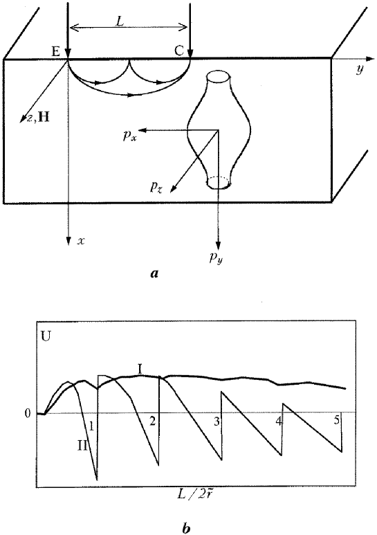
Figure 11: Experimental geometry (a) and the shape of the transverse ($\boldsymbol{L}\bot\boldsymbol{H}$) electron focusing signal (curve I) and its derivative with respect to $\boldsymbol{H}$ (curve II) in the case when the line $\boldsymbol{L}$ connecting the contacts on the same face of the sample and the magnetic field vector $\boldsymbol{H}$ lies in the plane of the layers.

2. The crystal surface bearing contacts coincides with a high-conductivity plane. In this case, a thin layer (whose thickness is of the order of $\tilde{r}\eta$) of “jumping” electron trajectories exists in a magnetic field $\boldsymbol{H}\bot p_{y}$ parallel to the boundary, in the transverse electron focusing geometry (Fig. 11a), such electrons ensure a ballistic transport of charge between point contacts arranged at the same face of the crystal, and the function $A$ is defined by relations (5.15). In the case under investigation, the values of a magnetic field for which the separation between contacts is multiple to the maximum jump over the surface are preferred [60, 61], i.e.,

$$L=\frac{2\pi hnc}{eH_{n}a},\quad(n=1,2,\ldots).$$ (5.30)

For $H=H_{n}$, the $U(H)$ dependence has kinks rather than extrema (curve 1in Fig. 11b) since electrons having the maximum displacement along the surface over a period approach the surface at small angles, and their contribution to the emf measured by collector is small in accordance with Equation (5.7). In the Fermi surface model (2.21) in which the cross section $p_{z}=\mbox{const}$ does not contain extremal diameters (and hence ordinary electron focusing peaks are absent), the partial amplitude $A$ for $\boldsymbol{H}\bot\boldsymbol{L}$ and $H\neq H_{n}$ is given by

$$A=\mu^{2}\frac{\zeta^{2}_{n}\sin\pi\zeta_{n}}{2F(\sqrt{\eta},\pi\zeta_{n}/2)\sqrt{1-\eta\sin^{2}(\pi\zeta_{n}/2)}},\quad\zeta_{n}<1,$$ (5.31)

where

$$\zeta_{n}=\frac{L}{2n\tilde{r}};\quad\tilde{r}=\frac{\pi hc}{eHa};\quad n\geq n_{0};\quad\zeta_{n_{0}}<1;\quad\zeta_{n_{0}-1}>1.$$

The contribution of electrons, sliding along the surface with a small velocity component normal to the boundary, cannot be described by Equation (5.15) and must be taken into account with the help of the next approximation in the small parameter $\mu$:

$$A^{\rm max} = \frac{\sqrt{\pi}(2\pi\hbar/a)}{\langle v_{x}\Theta(-v_{x})\rangle}\mu^{3}\frac{\dot{v}_{x}L}{nv_{y}^{2}(\partial^{2}S/\partial p_{z}^{2})}$$ (5.32)

$$= \pi^{-3/2}\mu^{3}\frac{1}{K(\eta)\sqrt{1-\eta}},\quad v_{x}=0,\zeta_{n}=1,$$

where $K(k)$, $F(k,\varphi)$ are complete and incomplete elliptic integrals of the first kind. The dot in Equation (5.23) denotes the differentiation of electron velocity of motion along the trajectory with respect to time. All the Fermi surface characteristics in Equation (5.23) are taken at the point $\boldsymbol{p}_{0}$ at which

$$v_{x}(\boldsymbol{p}_{0})=v_{z}(\boldsymbol{p}_{0})=0.$$ (5.33)

Apparently, it would be more convenient in this case to investigate experimentally the derivative $\partial U/\partial H$ of the electron focusing signal with respect to a magnetic field, which has jumps at the values $H_{n}$ determined by Equation (5.21). Figure 11b shows the magnetic field dependence of the electron focusing signal (curve 1) and its derivative (curve 2) for the simple model of the Fermi surface (2.21).

In a magnetic field orthogonal to the crystal surface, electrons injected by the emitter move along helical trajectories to the bulk of the crystal. Setting the collector and emitter at opposite faces of a thin plate and directing the vector $\boldsymbol{H}$ along the line connecting the contacts, we can observe the effect of the longitudinal electron focusing (Fig. 12a). It can be seen that with such a geometry, only the electrons for which the time of motion $\Delta T=L/\bar{v}_{z}$ is a multiple of their period of motion in a magnetic field ($\Delta T=kT_{\rm H}$; $k=1,2,\ldots$) can get from contact to contact.

The peaks of the longitudinal electron focusing signal correspond to the value of the field at which electrons have the extremal value of the time-averaged velocity component $\bar{v}_{z}$:

$$H_{n}=\frac{kc}{eL}\left(\frac{\partial S}{\partial p_{z0}}\right)_{\rm extr},$$ (5.34)

where

$$p_{z0}=-\frac{\pi\hbar}{2a}\left(\frac{\partial S}{\partial p_{z0}}\right)_{\rm extr}$$

is the extremal value of the derivative of the Fermi surface cross-sections perpendicular to the axis.

In the case when the Fermi surface (1.1) is a body of revolution, we obtain the following expression for the partial amplitude:

$$A = \frac{m^{*}m_{zz}v_{z}^{2}}{\langle v_{z}\Theta(v_{z})\rangle}$$ (5.38)

$$\times \left\{\begin{array}[]{ll}\displaystyle\sqrt{\pi}\mu\frac{v_{z}}{v_{\bot}},&\displaystyle\frac{\partial v_{z}}{\partial p_{z0}}=m^{-1}_{zz}\neq 0;\\[8.0pt] \displaystyle\frac{1}{2}\Gamma\left(\frac{1}{4}\right)\mu^{1/2}\left(\frac{a}{\hbar}m_{zz}\sqrt{v_{\bot v_{z}}}\right)^{-1},&\displaystyle\frac{\partial v_{z}}{\partial p_{z0}}=m^{-1}_{zz}=0,\\[8.0pt] &\displaystyle p_{z0}=-\frac{\pi\hbar}{2a}\end{array}\right.$$

where

$$v_{\bot}=\sqrt{v_{x}^{2}+v_{y}^{2}};\quad m^{*}=\frac{1}{2\pi}\frac{\partial S}{\partial\varepsilon_{p}}.$$

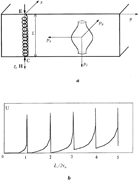
Figure 12: Experimental geometry (a) and the shape of the longitudinal ($\boldsymbol{L}\|\boldsymbol{H}$) electron focusing peaks (b) in the case when the line $\boldsymbol{L}$ connecting the contacts on the same face of the crystal and the magnetic field vector $\boldsymbol{H}$ is orthogonal to the plane of the layers.

If the function $\varepsilon_{0}$ is quadratic and isotropic. Equation (5.26) can be transformed to

$$A=\sum\limits_{k=k_{0}}^{\infty}\left\{\begin{array}[]{ll}\displaystyle\frac{\sqrt{\pi}}{2}\mu\frac{\varepsilon_{1}a}{v_{\rm F}\hbar}\frac{\lambda_{k}^{3}}{[(1-\eta\sqrt{1-\lambda_{k}^{2}})(1-\lambda_{k}^{2})]^{1/2}},&\lambda_{k}<1;\\[8.0pt] \displaystyle\frac{\Gamma(1/4)}{4}\mu^{1/2}\left(\frac{a\varepsilon_{1}}{\hbar v_{\rm F}}\right)^{1/2},&\lambda_{k}=1\end{array}\right.$$ (5.40)

where

$$\lambda_{k}=\frac{L}{2\pi kr_{0}};\quad r_{0}=\frac{\varepsilon_{1}aT_{\rm H}}{2\pi\hbar};\quad\lambda_{k_{0}}<1;\quad\lambda_{k_{0}-1}>1.$$

The time of motion along the trajectory for an electron reaching the collector over $k$ complete periods is $\Delta T=Lh/\varepsilon_{1}a\lambda_{k}$. The explicit form of the magnetic field dependence for the longitudinal electron focusing signal can be easily obtained, if we substitute Equation (5.27) into Equation (5.12) and put $n_{0}=N=1$ in it. The results of numerical calculations are presented in Fig. 12b.

Thus, the magnetic field dependence $U(H)$ of the electron focusing signal in the layered conductors is determined by the size of the point contacts and their orientation, relative to crystallographic axes. If the contacts are arranged on the crystal surface perpendicular to the layers with a high electrical conductivity, electron focusing can be observed only in a magnetic field directed along this surface. Setting both of the point contacts at the same sample boundary, we can determine the diameters of closed Fermi surface cross-sections from the positions of transverse electron focusing peaks on the magnetic field scale. The shape of the lines ($U(H)$ dependence) depends significantly on the relation between two small parameters: the ratio $\eta$ of the conductivity across the layers to the conductivity in the layers-plane and the ratio $\mu$ of the diameter of contacts to the separation between them.

In the case when vector $\boldsymbol{H}$ lies in the layers-plane, the electrons injected by emitter are displaced along an open trajectory to the bulk of the sample. In the thin plate (the thickness of which is much smaller than the mean free path), such electrons can be focused by a magnetic field at the collector arranged on the sample face opposite to the emitter. However, electron focusing in such geometry can be observed only for very small contacts for which $\mu\ll\eta$.

If the plane of the surface bearing the contacts is parallel to high conductivity layers, and the magnetic field is orthogonal to the Fermi surface axis electrons belonging to open Fermi surface cross sections move along periodic trajectories along the crystal boundary. For values of the field $H$ corresponding to the separation between the electrodes that are multiple of the electron displacement in an open trajectory over period $T_{\rm op}$, the derivative $\mbox{d}U/\mbox{d}H$ of the electron focusing signal undergoes jumps. The presence of singularities in the derivative $\mbox{d}U/\mbox{d}H$ and not in the signal $U(H)$ can be explained by the fact that electrons, for which the time between two consecutive collisions with the boundary is close to $T_{\rm op}$, reach the collector at small angles and their contribution to $U(\boldsymbol{H})$ is small.

The effect of longitudinal electron focusing can be observed in a magnetic field orthogonal to the surface. The values of $H$ for which the signal $U(\boldsymbol{H})$ has peaks can be used for determining the extremal value of the electron velocity along the Fermi surface cylinder axis.

Thus, the electron focusing in the layered organic metals being a source of information on their Fermi surface, enable us to obtain, along with the extremal diameters and velocities, the period of constant energy surfaces in the direction of the “openness”. Another important advantage of the electron focusing is the applicability of this method to the analysis of surface scattering of electron.

5.2 Resistance of Point-Contact between Layered Conductors

Two bulk metallic electrodes, contacting one another (contiguously) over a small area, form an electrical contact of small dimensions – a point contact. When an electric current is passed through such a system, it is concentrated in a narrow region (system with concentration of current), reaching densities of $10^{13}$–$10^{14}$ A/m². The metal in this narrow region is not overheated due to the effective heat flow to the banks (the electrodes) of the contact, provided that mean free path for energetic relaxation of electrons $l_{\varepsilon}$ is greater than the characteristic (the largest) dimension of the narrow region. Two possible asymptotic regimes can be distinguished for the electric current through a point contact: the ballistic regime (clean conductor) when the mean free path for elastic relaxation $l_{i}$ is much greater than $d$ and the diffusion regime (impure conductor) when $l_{i}\ll d$ (where $d$ is the characteristic dimension of the contact).

Let us consider a junction in the form of a single – sheet hyperboloid of revolution (Fig. 13a)

$$F(x_{1},x_{2},x_{3})=\frac{\rho^{2}}{\nu^{2}}-\frac{x_{3}^{2}}{\beta^{2}}-1=0$$ (5.41)

subjected to a voltage $V$ and placed in a magnetic field $\boldsymbol{H}$ directed at an angle $\theta$ with respect to the $x_{3}$-axis ($\rho^{2}=x_{1}^{2}+x_{2}^{2}$) This model allows us to examine the limiting cases: the model of aperture with an infinitely thin flat partition, dividing the two metallic half-spaces ($\beta\to 0$) (see Fig. 13b) and the model of a long channel (the length of the channel is much larger than its diameter $d=2\nu$), filled with metal and connecting the bulk metallic banks ($\nu\to 0$).

In the semiclassical approximation the current

$$\boldsymbol{I}=\frac{2e^{2}}{(2\pi\hbar)^{3}}\int\limits_{S_{\rm c}}\int\mbox{d}^{3}\boldsymbol{p}\,\boldsymbol{v}f(\boldsymbol{p})$$ (5.42)

flowing through a contact area $S_{\rm c}=\pi\nu^{2}$ should be determined by means of the nonequilibrium electron-distribution function $f(\boldsymbol{p},\boldsymbol{r})$ satisfying the Boltzman equation (2.2).

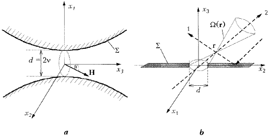
Figure 13: A model of the point-contact in the form of a single-sheet hyperboloid of revolution (a); its limiting case ($\beta=0$) is a circular orifice (b); $\Omega(\boldsymbol{r})$ is the solid angle within which velocities of the electrons passing the contact along the ballistic trajectories fit.

In the zeroth approximation in electron–phonon collision integral, the distribution function $f(\boldsymbol{p},\boldsymbol{r})=f_{\boldsymbol{p}}^{(0)}(\boldsymbol{r})$ can be presented in the form [70]

$$f_{\boldsymbol{p}}^{(0)}(\boldsymbol{r}) = \alpha_{\boldsymbol{p}}(\boldsymbol{r})f_{0}\left(\varepsilon(\boldsymbol{p})+e\Phi(\boldsymbol{r})-\frac{eV}{2}\right)$$ (5.43)

$$+ (1-\alpha_{\boldsymbol{p}}(\boldsymbol{r}))f_{0}\left(\varepsilon(\boldsymbol{p})+e\Phi(\boldsymbol{r})+\frac{eV}{2}\right),$$

where $f_{0}$ is the Fermi distribution function, $\Phi(\boldsymbol{r})$ is the electrical potential, and $\alpha_{\boldsymbol{p}}(\boldsymbol{r})$ signifies the probability for an electron with the momentum $\boldsymbol{p}$ to arrive at the point $\boldsymbol{r}$ from $+\infty$. For $eV\ll\varepsilon_{\rm F}$, the function $\alpha_{\boldsymbol{p}}(\boldsymbol{r})$ satisfies a field-independent kinetic equation which, for the sake of simplicity, can be written in the approximation of the mean relaxation time $\tau$

$$\frac{\partial\alpha_{\boldsymbol{p}}(\boldsymbol{r})}{\partial t}+\frac{\alpha_{\boldsymbol{p}}-\alpha}{\tau}=0.$$ (5.44)

The boundary condition to Equation (5.31) ensures that the current does not flow through the surface $\Sigma$

$$\alpha_{\boldsymbol{p}}(\boldsymbol{r})=\alpha_{\tilde{\boldsymbol{p}}}(\boldsymbol{r}),\quad\boldsymbol{r}\in\Sigma$$ (5.45)

and that equilibrium is restored in the electron subsystem at the contact banks $|\boldsymbol{r}|\to\infty$

$$\alpha_{\boldsymbol{p}}(\boldsymbol{r}\to\infty)=\Theta(x_{3}).$$ (5.46)

The momenta $\boldsymbol{p}$ and $\tilde{\boldsymbol{p}}$ satisfy Equations (5.3). In order to avoid cumbersome calculations, we shall consider the specular reflection of electrons at the boundary (Equation (5.32)).

Here

$$\alpha(\boldsymbol{r},\boldsymbol{H})=\frac{\langle\alpha_{\boldsymbol{p}}\rangle}{\langle 1\rangle};\quad\langle\ldots\rangle=\frac{eH}{c}\int\limits_{\varepsilon(\boldsymbol{p})=\varepsilon_{\rm F}}\mbox{d}t\,\mbox{d}p_{\rm H}\,\ldots\,,$$ (5.47)

$t$ is, as below, the time of the electron motion along its trajectory in a magnetic field, and $p_{\rm H}$ is the momentum projection on the direction of the vector $\boldsymbol{H}$. The integration in Equation (5.34) is carried out over the open constant-energy surface within the limits of the Brillouin zone.

The distribution of the electric potential $\Phi(\boldsymbol{r})$ in a sample satisfies the Poisson equation which can be reduced to the electroneutrality condition (3.15) if a Debye screening radius is small in comparison with the contact diameter. It was shown in [70, 71] that having the probability $\alpha_{\boldsymbol{p}}(\boldsymbol{r})$ determined, we can calculate the contact resistance for low voltages ($V\to 0$)

$$R^{-1}=\frac{I}{V}=\frac{2e^{2}}{(2\pi\hbar)^{3}}\int\limits_{S_{\rm c}}\mbox{d}S\,\langle\boldsymbol{v}\alpha_{\boldsymbol{p}}\rangle,$$ (5.48)

and the electrical potential distribution

$$\Phi(\boldsymbol{r})=\frac{V}{2}(2\alpha(\boldsymbol{r},\boldsymbol{H})-1).$$ (5.49)

The solution of Equation (5.31) can be formally presented as

$$\alpha_{\boldsymbol{p}}(\boldsymbol{r},\boldsymbol{H})=\frac{1}{\tau}\int\limits_{-\infty}^{t}\mbox{d}t^{\prime}\,\exp\left(\frac{t-t^{\prime}}{\tau}\right)\alpha(\boldsymbol{r}-\boldsymbol{r}(t)+\boldsymbol{r}(t^{\prime})).$$ (5.50)

If the electric potential, and hence (in view of Equation (5.36)) the mean probability $\alpha$, varies smoothly at distances comparable with the characteristic size $\boldsymbol{r}(t)-\boldsymbol{r}(t-\tau)$ of the electron trajectory in the corresponding direction, the integral equation (5.37) for $\alpha_{\boldsymbol{p}}(\boldsymbol{r})$ can be replaced by a differential equation for its mean value $\alpha$. We expand $\alpha(\boldsymbol{r}-\boldsymbol{r}(t)+\boldsymbol{r}(t^{\prime}))$ in the integral in Equation (5.37) into a series near the point $\boldsymbol{r}(t)=\boldsymbol{r}(t^{\prime})$:

$$\alpha_{\boldsymbol{p}}(\boldsymbol{r}) = \alpha-\frac{\partial\alpha}{\partial\boldsymbol{r}}$$

$$+ \frac{\partial^{2}\alpha}{\partial x_{i}\partial x_{k}}\int\limits_{-\infty}^{t}\mbox{d}t^{\prime}\,\exp\left(\frac{t-t^{\prime}}{\tau}\right)v_{i}(t^{\prime})(x_{k}(t)-x_{k}(t^{\prime}))\ldots\,,$$

$$g(\boldsymbol{p},\boldsymbol{H}) = \int\limits_{-\infty}^{t}\mbox{d}t^{\prime}\exp\left(\frac{t-t^{\prime}}{\tau}\right)\boldsymbol{v}(t^{\prime}).$$ (5.52)

Averaging Equation (5.38) over the directions of the momentum $\boldsymbol{p}$ and going over to dimensionless variables

$$x_{i}^{\prime}=\frac{2x_{i}}{d}\left(\frac{\sigma_{33}}{\sigma_{ii}}\right)^{1/2}$$ (5.53)

we obtain the following equation for $\alpha(\boldsymbol{r},\boldsymbol{H})$

$$\Delta\alpha(\boldsymbol{r}^{\prime})+\sum\limits_{i\neq k}C_{ik}^{(\rm s)}\frac{\partial^{2}\alpha}{\partial x_{i}^{\prime}\partial x_{k}}=0,$$ (5.54)

where

$$C_{ik} = \frac{\sigma_{ik}}{\sqrt{\sigma_{ii}\sigma_{kk}}},$$ (5.55)

$$\sigma_{ik} = \frac{2e^{2}}{(2\pi\hbar)^{3}}\langle v_{i}g_{k}\rangle$$ (5.56)

are the electrical conductivity tensor components in a bulk conductor and $C_{ik}^{(\rm s)}$ is the symmetric part of $C_{ik}$ (5.42). Equation (5.41), which coincides with the continuity equation $\div\boldsymbol{j}=0$, must be supplemented by boundary conditions. Using Equations (5.32) and (5.33), we obtain

$$\alpha(\boldsymbol{r}\to\infty) = \Theta(x_{3});$$ (5.57)

$$\boldsymbol{n}^{\prime}\nabla\alpha(\boldsymbol{r}^{\prime})+\sum\limits_{i\neq k}n_{i}^{\prime}C_{ik}\left.\frac{\partial\alpha}{\partial x_{k}^{\prime}}\right|_{\boldsymbol{r^{\prime}}\in\Sigma^{\prime}} = 0,$$ (5.58)

($\boldsymbol{n}^{\prime}=\nabla F(\boldsymbol{r}^{\prime})/|\nabla F(\boldsymbol{r}^{\prime})|$ is the vector normal to the metal boundary $\Sigma^{\prime}$ (5.28)) in coordinates (5.40). The solution of boundary-value problem (5.41), (5.44), (5.45) would lead to a rigorous criterion for the applicability of the expression (5.38) for the function $\alpha_{\boldsymbol{p}}(\boldsymbol{r})$. In spite of the considerable simplification due to making use of the representation (5.38) for the function $\alpha_{\boldsymbol{p}}(\boldsymbol{r})$, the problem of evaluating the electric field in a metal remains quite complicated and can be solved analytically only if the coefficients $C_{ik}$ are small. In the main approximation ($C_{ik}=0$) the boundary value problem (5.41)–(5.45) is reduced to the Neumann’s problem with zeroth boundary condition for the normal derivative $\partial\alpha/\partial n^{\prime}$ on the hyperboloid surface (5.28) which is no longer a figure of revolution in coordinates (5.40). For this reason, it is convenient to solve the Equation (5.41) by going to the general ellipsoidal coordinates $\xi$, $\eta$, $\zeta$

$$(x_{1}^{\prime})^{2} = \frac{(a^{2}+\xi)(a^{2}+\eta)(a^{2}+\zeta)}{(a^{2}-b^{2})a^{2}};$$

$$(x_{2}^{\prime})^{2} = \frac{(b^{2}+\xi)(b^{2}+\eta)(b^{2}+\zeta)}{(b^{2}-a^{2})b^{2}};$$

$$(x_{3}^{\prime})^{2} = \frac{\xi\eta\zeta}{a^{2}b^{2}};$$ (5.59)

$$-a^{2}\leq\zeta\leq-b^{2};\quad-b^{2}\leq\eta\leq 0;\quad\xi\geq 0;$$

$$a^{2}=c_{1}^{2}+\varkappa^{2};\quad b^{2}=c_{2}^{2}+\varkappa^{2};\quad c_{i}^{2}=\frac{\sigma_{33}}{\sigma_{ii}};\quad\varkappa=\frac{\beta}{\nu}.$$

For the sake of definiteness, we suppose that $\sigma_{11}\leq\sigma_{22}$ and hence $a\geq b$. In these coordinates the contact surface corresponds to $\eta=-\varkappa^{2}$, and we obtain for the probability $\alpha(\boldsymbol{r}^{\prime})$:

$$\alpha(\boldsymbol{r}^{\prime})=\Theta(z^{\prime})-\frac{1}{2K(k)}\mbox{sign}\,(x_{3}^{\prime})F\left(\arctan\frac{a}{\sqrt{\xi}},k\right),$$ (5.60)

where $F(\phi,k)$ and $K(k)$ are incomplete and complete elliptical integrals of the first kind, $k^{2}=1-b^{2}/a^{2}$.

Substituting the expansion (5.38) and the function $\alpha$ (5.45) into Equation (5.35) for the electric current, we have the final result for the resistance [72,7 3]:

$$R^{-1}(h)=\sqrt{\sigma_{11}\sigma_{22}}\mbox{d}a\Psi(\phi,k).$$ (5.61)

Here,

$$\Psi(\phi,k)=F(\phi,k^{\prime})\left[\frac{\boldsymbol{E}(k)}{\boldsymbol{K}(k)}-1\right]+E(\phi,k^{\prime})-\frac{\varkappa}{a}\frac{c_{2}}{c_{1}}$$

$$k^{\prime}=\sqrt{1-k^{2}};\quad\phi=\arcsin\left(\frac{ac_{1}^{2}}{bc_{2}^{2}}\right);\quad d=2\nu$$ (5.62)

and $\boldsymbol{E}(k)$ is a complete elliptic integral of the second kind.

Let us first consider the case when $\boldsymbol{H}=0$ and a contact is formed by conductors with the small elastic mean free path ($l_{i}\ll d$). In this case the function $\boldsymbol{g}(\boldsymbol{p},\boldsymbol{H}=0)$ can be written in the form:

$$\boldsymbol{g}(\boldsymbol{p})=\tau\boldsymbol{v}.$$ (5.63)

In the absence of a magnetic field the conductivity tensor (5.43) is diagonal and (5.47) is the exact solution of Equation (5.41). Using the expression (5.47) for the probability $\alpha$ we can write the resistance for a point contact in the form of aperture $r^{2}=x_{1}^{2}+x_{2}^{2}\leq d^{2}/4$ of diameter $d$ in a plane of insulating partition ($\beta=\varkappa=0$) (see Fig. 13b) as

$$R^{-1}(0)=\frac{\pi}{2}\sqrt{\sigma_{11}\sigma_{22}}\mbox{d}K^{-1}\left(\sqrt{1-\left(\frac{\sigma_{22}}{\sigma_{11}}\right)^{2}}\right);\quad\sigma_{11}\geq\sigma_{22}.$$ (5.64)

Equation (5.51) indicates that the point contact resistance

$$R^{-1}=\left\{\begin{array}[]{ll}d\sqrt{\sigma_{\bot}\sigma_{\|}};&\sigma_{33}=\sigma_{\bot};\;\sigma_{11}=\sigma_{22}=\sigma_{\|},\\[6.0pt] \displaystyle\pi\mbox{d}\sigma_{\|}\ln^{-1}\left(\frac{\sigma_{\|}}{\sigma_{\bot}}\right);&\displaystyle\sigma_{33}=\sigma_{11}=\sigma_{\|};\;\sigma_{22}=\sigma_{\|};\;\frac{\sigma_{\|}}{\sigma_{\bot}}\gg 1,\end{array}\right.$$ (5.65)

where

$$\sigma_{\bot}=\frac{e^{2}\tau m\pi\varepsilon_{1}^{2}a}{(2\pi)^{3}\hbar^{4}};\quad\sigma_{\|}=\frac{8\pi^{2}e^{2}\tau\varepsilon_{\rm F}}{(2\pi\hbar)^{2}a}\left(1-\frac{\varepsilon_{1}}{\varepsilon_{\rm F}}\right),$$

depends not only on the electrical conductivity along the contact axis, but also on the conducting properties of the sample in the direction perpendicular to this axis. This is due to the three-dimensional nature of current flow in the point-contact region. It should be noted that for $\sigma_{33}=\sigma_{\|}$ and $(\sigma_{\|}/\sigma_{\bot})\to\infty$ (strictly two-dimensional conductivity), the resistance (5.52) contains the logarithmic divergence. In this case we must take into account the sample size $D$, and for $(\sigma_{\|}/\sigma_{\bot})\gg(D/d)\gg 1$ the resistance is $R(0)\sim(\sigma_{\|}d)^{-1}\ln(D/d)$.

In pure metals the ballistic mode of current flow through the contact, for which $d\ll l_{i}$ can be realized. In this case we can discount the second term in Equation (5.31). Its solution is $\alpha=\mbox{const}(t)$. Using the boundary condition (5.33) we found $\alpha_{\boldsymbol{p}}(\boldsymbol{r})$ for the contact in the form of aperture

$$\alpha_{\boldsymbol{p}}(\boldsymbol{r})=\Theta(\boldsymbol{v}\in\Omega(\boldsymbol{r}));\quad x_{2}<0,$$ (5.66)

where $\Omega(\boldsymbol{r})$ is the solid angle enclosing the velocities of electrons passing through the aperture and the point $\boldsymbol{r}$ (see Fig. 13b).

Substituting the solution (5.53) into Equation formula (5.35), we obtain the following expression for the resistance:

$$R^{-1}(0)=\left\{\begin{array}[]{ll}\displaystyle\frac{1}{4\pi^{2}}\sigma_{\|}\frac{S_{\rm c}}{l_{i}}\boldsymbol{E}\left(\sqrt{\frac{\varepsilon_{1}}{\varepsilon_{\rm F}}}\right);&\sigma_{33}=\sigma_{11}=\sigma_{\|};\;\sigma_{22}=\sigma_{\bot},\\[8.0pt] \displaystyle\sqrt{\frac{\pi\sigma_{\bot}\sigma_{\|}}{2}}\frac{S_{\rm c}}{l};&\sigma_{33}=\sigma_{\bot};\;\sigma_{11}=\sigma_{22}=\sigma_{\|}.\end{array}\right.$$ (5.67)

It is interesting to note that, according to Equations (5.52) and (5.54), the ratio $R_{\|}/R_{\bot}$ for $\varepsilon_{1}\ll\varepsilon_{\rm F}$ is inversely proportional to the square root of the ratio $\sigma_{\|}/\sigma_{\bot}$ and depends weakly on the relation between the contact diameter $d$ and the electron mean free path $l_{i}$ ($R_{\|}$, $\sigma_{\|}$ and $R_{\bot}$, $\sigma_{\bot}$ are the resistances and the conductivities of the contact with the axis oriented parallel and perpendicular to the layers, respectively).

Thus, the electrical conductivity of the point contact between layered metals is extremely sensitive to the orientation of the crystals in the contact. However, in contrast to the case of a bulk sample, the resistance depends on the metal conductivity in the directions parallel and perpendicular to the contact axis in view of the three-dimensional nature of current flow.

In a strong magnetic field ($\gamma_{0}=cp_{\rm F}/eHl_{i}\ll 1$, $p_{\rm F}$ is the Fermi momentum) the function $\boldsymbol{g}(\boldsymbol{p},\boldsymbol{H})$, appearing in the theory of galvanomagnetic phenomena [69], can be presented in the form of a power series in $1/H$ whose first terms are given by

$$g_{x} = -\frac{c}{eH}(p_{y}\cos\theta-p_{z}\sin\theta);$$

$$g_{y} = v_{\rm H}\tau\sin\theta-\frac{cp_{x}}{eH}\cos\theta;$$

$$g_{z} = \frac{cp_{y}}{eH}\sin\theta+v_{\rm H}\tau\cos\theta,$$ (5.68)

for closed electron orbits ($\gamma=\gamma_{0}\sec\theta\ll 1$, $\boldsymbol{H}=(0,H\sin\theta,H\cos\theta)$) and

$$g_{x}=\frac{c}{eH}(p_{y}-\bar{p}_{y});\quad g_{y}=\bar{v}_{y}\tau;\quad g_{z}=v_{z}\tau$$ (5.69)

for open electron orbits ($\theta=\pi/2$, $\gamma_{0}\ll 1$). In Equations (5.55), (5.56) $v_{\rm H}=\partial\varepsilon(\boldsymbol{p})/\partial p_{\rm H}$ and the bar indicates the value of a function averaged over the period of motion in a magnetic field. In following analysis we shall assume that $\eta\ll\gamma$ and the inclination $\theta$ of the magnetic field does not coincide with the value $\theta_{\rm c}$ for which the conductivity across the layers decreases considerably ($\sigma_{zz}(\theta_{\rm c})\approx\eta^{4}$, see Equations (2.33)). In this case, as it follows from Equations (2.27), and (5.42), the coefficients $C_{xz}$ and $C_{yz}$ are small and the terms containing these coefficients in Equation (5.41) can be omitted. Since the anisotropy of conductivity in the layers-plane is usually not significant, unjustifiably cumbersome formulas can be avoided by assuming that the Fermi surface is a figure of revolution. It was shown for this case (see Equations (2.24), (2.27)) that if the inequality $\eta\ll\gamma$ is satisfied, then $\sigma_{xx}\approx\sigma_{yy}=\sigma_{\|}(H)$ for any angle $\theta$, while for $\theta=\pi/2$ we have $\sigma_{xy}=\sigma_{yz}=0$. The inequality $\eta\ll\gamma$, which is violated only in very strong fields, indicates that the conductivity across the layers always remains much lower than the conductivity along the layers.

We consider separately the two main geometries of the experiment.

1. Contact axis is perpendicular to the layers ($x_{3}=x$; $x_{2}=y$; $x_{3}=z$; $\sigma_{33}=\sigma_{zz}$; $\sigma_{11}=\sigma_{22}=\sigma_{\|}$) (see Fig. 14).

In Equation (5.46) and (5.47) we must replace

$$c_{1}^{2}=c_{2}^{2}=L^{2}=\frac{\sigma_{zz}}{\sigma_{\|}}<1.$$

The probability $\alpha$ can be presented in the form [71]:

$$\alpha(\boldsymbol{r})=\Theta(z)-\frac{1}{\pi}\mbox{sign}(z)\arctan\left(\frac{1}{\chi}\right).$$ (5.70)

where

$$\chi=\left\{\frac{r^{2}}{2\nu^{2}}-\frac{1}{2}+\left[\left(\frac{r^{2}}{2\nu^{2}}-\frac{1}{2}\right)^{2}+\frac{z^{2}L^{2}}{\nu^{2}}\right]^{1/2}\right\}^{1/2}\quad r=\sqrt{x^{2}+y^{2}}.$$ (5.71)

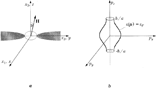
Figure 14: The model of the point (a) in the case when the contact axis coincides with the axis of the Fermi surface (b) of a layered conductor.

It follows from Equations (5.36), (5.57) that the characteristic scale of variation of the electric field along the $z$-axis is of the order of $d/(L^{2}+\varkappa^{2})^{1/2}$ (where $L^{2}=\sigma_{zz}/\sigma_{\|}$, $\varkappa=\beta/\nu$) and may be either larger or smaller than the contact diameter. Substituting the function $\alpha_{\boldsymbol{p}}(\boldsymbol{r})$ in the form (5.38) into the expression (5.35) for the resistance and taking into account the equalities (5.55) and (5.57), we obtain

$$R^{-1}(H)=\sqrt{\sigma_{zz}\sigma_{\|}}d\tan\psi;\quad\psi=\frac{1}{2}\arctan\left(\frac{L}{\varkappa}\right).$$ (5.72)

In view of the oscillatory dependence of $\sigma_{zz}$ on the slope of the magnetic field (Equation (2.33)), the magnetoresistance of the point contact is also a nonmonotonic function of $\theta$. It should be noted that $R(H)$ is highly sensitive to the contact geometry. Thus, for a constriction having a form close to aperture ($\varkappa\ll 1$), we have

$$R^{-1}(H)=\left\{\begin{array}[]{ll}\displaystyle\sigma_{zz}\frac{d^{2}}{4\beta};&1\gg\varkappa\gg L,\\[6.0pt] d\sqrt{\sigma_{zz}\sigma_{\|}};&1\gg L\gg\varkappa.\end{array}\right.$$ (5.73)

The magnetic field variation of the parameter $L^{2}(H)$, viz., the ratio of electrical conductivities across and along the layers, depends significantly on the orientation of the vector $\boldsymbol{H}$. If the vector $\boldsymbol{H}$ is parallel to the contact axis ($\sigma_{zz}(\boldsymbol{H})=\sigma_{\bot}=\mbox{const}(\boldsymbol{H})$), an increase in the field causes a decrease in the conductivity $\sigma_{\|}(H)$ and an increase in $L$. For $L(0)\ll\varkappa$, there exist a range of values of $H$ ($L(H)<\varkappa$) in which $R(H)=\mbox{const}$. Formally, such a situation corresponds to a contact in the form of strongly elongated channel, since, although the real contact length for $\varkappa\ll 1$ is much smaller than its diameter, the electron velocity along the channel axis is much lower than the velocity of diffusive motion along a normal to this axis of the Larmour orbit center. In stronger fields, when $L(H)$ becomes larger than the parameter $\varkappa$ characterizing the shape of the constriction, the quasi-two-dimensional current flow is replaced by the three-dimensional flow, and the contact resistance depends linearly on the magnetic field as in the case of an isotropic metal [13].

The magnetic field, which is orthogonal to the contact axis, suppresses the electric conductivity $\sigma_{zz}$ across the layers, leaving the in-plane conductivity $\sigma_{\|}$ practically unchanged. This corresponds to a decrease in parameter $L$ with increasing $H$. Hence for $L(0)\ll\varkappa$, the contact resistance in strong magnetic fields is proportional to $H^{2}$ for $\gamma_{0}\leq\eta^{1/2}$ (see Equation (2.14)). If, however, $L(0)\gg\varkappa$ (although $L(0)\simeq\eta\ll 1$), the quadratic dependence $R(H)$ is preceded by the linear magnetoresistance $L(H)>\varkappa$.

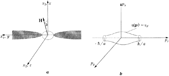
Figure 15: The model of the point-contact (a) in the case when the contact axis is parallel to the layers (b).

2. Contact axis is parallel to the layers ($x_{3}=x$) (Fig. 15).

If the magnetic field is perpendicular to the axis of the cylindrical Fermi surface, the coefficients $C_{ik}$ are small for any angle of inclination of the magnetic field to the contact axis. It follows from (5.48) that if the contact axis lies in the plane of a high electrical conductivity ($\sigma_{33}=\sigma_{\|}$) the resistance depends logarithmically on the magnetic field $H$ (except for the case of a strongly elongated constriction ($\varkappa\gg L^{-2}$), for which $R(H)=\mbox{const}$:

$$R^{-1}(H)=\sigma_{\|}d\left\{\begin{array}[]{ll}\displaystyle\arctan\left(\frac{1}{\varkappa}\right)\ln^{-1}\left(\frac{4}{\varkappa L}\right);&\varkappa L\ll 1,\\[8.0pt] \displaystyle\frac{1}{2\varkappa};&\varkappa L\gg 1.\end{array}\right.$$ (5.74)

Thus, the magnetic field dependence $R(H)$ of contacts oriented at a right angle to the layers with a high electrical conductivity is extremely sensitive to the shape of the constriction. If the square root of the ratio $\sigma_{\bot}/\sigma_{\|}=L^{2}$ is smaller than the ratio $\varkappa=\beta/\nu$ of the length of the contact to its radius, the longitudinal resistance ($\theta=0$, $\theta$ is the angle between the contact axis and vector $\boldsymbol{H}$) and is independent of a magnetic field while the transverse magnetoresistance ($\theta=\pi/2$) is proportional to $H^{2}$. If the opposite inequality $L\gg\varkappa$ is satisfied, the resistance increases linearly with $H$. A variation of the field changes the magnitude $L^{2}$ ($L^{2}$ decreases for $\theta=\pi/2$ and increases in all other cases), thus allowing two types of field dependence $R(H)$ for the same contact in different ranges of $H$. As the inclination of the vector $\boldsymbol{H}$ relative to the layers is changed, $R(\boldsymbol{H})$ becomes a nonmonotonic function of an angle. In the geometry of the experiment, when the contact axis and the vector $\boldsymbol{H}$ lie in the plane of the layers with a high conductivity, the resistance shows a logarithmic dependence on $\boldsymbol{H}$.

5.3 Point-Contact Spectroscopy of Electron–Phonon Interaction

The information about the electron–phonon interaction in layered conductors is of great importance for understanding the nature of the superconducting state and for analysis of transport phenomena in these materials. Point-contact spectroscopy is an effective and reliable method of studying electron–phonon interaction [74, 75, 68]. Point contact spectroscopy is based on a strong nonequilibrium in the electronic system only in a small region of space whose dimension is less than the inelastic mean free path of electrons. In a point contact the Fermi surface splits into two parts with maximum energies differing by the bias energy $eV$. Effectively, there are two electronic beams moving in opposite directions with energies differing at each point of space by exactly the bias energy. Electron–phonon scattering in contacts results in a back flow: some electrons are reflected after entering the constriction and do not contribute to the contact current. Each time the bias $eV$ equals the energy of particular phonon $\hbar\omega_{\boldsymbol{p}}$, the current decreases. When averaged over all phonons, these contributions result in a nonlinear current in the contact. This technique has been used recently for reconstructing the point-contact spectroscopy of the electron–phonon interaction in organic metals $\beta$-(BEDT-TTF)${}_{2}X$ ($X=I_{2}$, $I$Au$I$) [76–80]. The experiments carried out in [76–80] revealed that the form of the point contact spectrum depends to a considerable extent on the orientation of the contact axis relative to planes with a high electrical conductivity.

The inelastic process of the electron–phonon interaction can be taken into account in the collision integral

$$W^{\rm(ep)}_{\rm col}\{f(\boldsymbol{p})\}\!\! = \!\!\sum\limits_{k}\int\frac{\mbox{d}^{2}q}{(2\pi\hbar)^{3}}W_{\boldsymbol{q},k}\big{\{}[f(\boldsymbol{p}+\boldsymbol{q})(1-f(\boldsymbol{p}))(N_{\boldsymbol{q},k}+1)$$ (5.75)

$$- \!\!f(\boldsymbol{p})(1-f(\boldsymbol{p}+\boldsymbol{q}))N_{\boldsymbol{q},k}]$$

$$\times \!\!\delta(\varepsilon(\boldsymbol{p}+\boldsymbol{q})-\varepsilon(\boldsymbol{p})-\omega_{\boldsymbol{q},k})$$

$$+ \!\![f(\boldsymbol{p}-\boldsymbol{q})(1-f(\boldsymbol{p}))N_{\boldsymbol{q},k}$$

$$- \!\!f(\boldsymbol{p})(1-f(\boldsymbol{p}-\boldsymbol{q}))(N_{\boldsymbol{q},k}+1)]$$

$$\times \!\!\delta(\varepsilon(\boldsymbol{p}-\boldsymbol{q})-\varepsilon(\boldsymbol{p})+\omega_{\boldsymbol{q},k})\big{\}}.$$

Here, the summation is carried out over the numbers $k$ of the phonon spectrum branches $\omega_{\boldsymbol{q},k}$; $W_{\boldsymbol{q},k}$ is the square of the magnitude of the electron–phonon interaction matrix element. In general, the system of Equations (2.2), (3.15) must be supplemented by the kinetic equation for determining the phonon distribution function $N_{\boldsymbol{q},k}$. But usually the state of the phonon system in the contact does not influence the form of the point contact spectra so much. This is so in the case of weak phonon–electron scattering, when the phonon distribution function $N_{\boldsymbol{q},k}$ is independent of bias, $V$ [81]. In the following consideration we shall assume that phonons are in thermal equilibrium, i.e.

$$N_{\boldsymbol{q},k}=\left(\exp\left(\frac{h\omega_{\boldsymbol{q},k}}{T}\right)-1\right)^{-1}.$$

We should write [70, 71] the particular solution $f_{\boldsymbol{p}}^{(1)}(\boldsymbol{r})$ of the non-homogeneous Equation (2.2) using the corresponding Green’s function $g_{\boldsymbol{pp}^{\prime}}(\boldsymbol{r},\boldsymbol{r}^{\prime})=g_{-\boldsymbol{p}^{\prime},-\boldsymbol{p}}(\boldsymbol{r}^{\prime},\boldsymbol{r})$:

$$f_{\boldsymbol{p}}^{(1)}(\boldsymbol{r})=\int\mbox{d}\boldsymbol{p}^{\prime}\,\mbox{d}\boldsymbol{r}^{\prime}\,g_{\boldsymbol{pp}^{\prime}}(\boldsymbol{r},\boldsymbol{r}^{\prime})W^{\rm(ep)}_{\rm col}\{f_{\boldsymbol{p}}^{(0)}(\boldsymbol{r}^{\prime})\},$$ (5.76)

where $f_{\boldsymbol{p}}^{(0)}(\boldsymbol{r})$ is the distribution function (5.30) in zeroth approximation in electron–phonon collision integral. The function $g_{\boldsymbol{pp}^{\prime}}(\boldsymbol{r},\boldsymbol{r}^{\prime})$ must be determined from the relations

$$\boldsymbol{v}^{\prime}\frac{\partial}{\partial\boldsymbol{r}^{\prime}}g_{\boldsymbol{pp}^{\prime}}(\boldsymbol{r},\boldsymbol{r}^{\prime})-\frac{1}{\tau}\{g_{\boldsymbol{pp}^{\prime}}-\langle g_{\boldsymbol{pp}^{\prime}}\rangle\} = -\delta(\boldsymbol{p}-\boldsymbol{p}^{\prime})$$ (5.77)

$$- \delta(\boldsymbol{r}-\boldsymbol{r}^{\prime});$$

$$g_{\boldsymbol{pp}^{\prime}}(\boldsymbol{r},\boldsymbol{r}^{\prime}\to\infty) = 0;$$ (5.78)

$$g_{\boldsymbol{pp}^{\prime}}(\boldsymbol{r},\boldsymbol{r}^{\prime}\in\Sigma) = g_{\boldsymbol{p}\tilde{\boldsymbol{p}}^{\prime}}(\boldsymbol{r},\boldsymbol{r}^{\prime}\in\Sigma).$$ (5.79)

Substituting the value $f_{\boldsymbol{p}}^{(1)}(\boldsymbol{r})$ in formula (5.29) we will get the expression for the change in the electric current $\Delta I$ due to the electron phonon interaction

$$\Delta I=\frac{2e}{(2\pi h)^{3}}\int\mbox{d}\boldsymbol{p}\,\mbox{d}\boldsymbol{r}\,G_{\boldsymbol{p}}(\boldsymbol{r})W^{\rm(ep)}_{\rm col}\{f_{\boldsymbol{p}}^{(0)}(\boldsymbol{r}^{\prime})\},$$ (5.80)

where

$$G_{\boldsymbol{p}}(\boldsymbol{r})=\int\mbox{d}S\,n_{3}\int\mbox{d}\boldsymbol{p}^{\prime}\,\mbox{d}v_{3}^{\prime}\,g_{\boldsymbol{p}^{\prime}\boldsymbol{p}}(\boldsymbol{r},\boldsymbol{r}^{\prime}).$$ (5.81)

Multiplying Equation (5.64) by $v_{3}$ and integrating it over the contact area $S_{\rm c}$ and momentum $\boldsymbol{p}$ we get the following equation and the boundary conditions for the function $G_{\boldsymbol{p}}(\boldsymbol{r})$

$$\boldsymbol{v}\frac{\partial}{\partial\boldsymbol{r}}G_{\boldsymbol{p}}(\boldsymbol{r})-\frac{1}{\tau}\{G_{\boldsymbol{p}}(\boldsymbol{r})-\langle G_{\boldsymbol{p}^{\prime}}(\boldsymbol{r})\rangle\} = -\delta(x_{3}),$$ (5.82)

$$G_{\boldsymbol{p}}(\boldsymbol{r}\to\infty) = 0,$$ (5.83)

$$G_{\boldsymbol{p}}(\boldsymbol{r}\in\Sigma) = G_{\tilde{\boldsymbol{p}}^{\prime}}(\boldsymbol{r}\in\Sigma).$$ (5.84)

The probability $\alpha_{\boldsymbol{p}}(\boldsymbol{r})$ satisfies the Equations (5.31)–(5.33), which combined with Equations (5.69)–(5.71) yield the relation [70]

$$G_{\boldsymbol{p}}(\boldsymbol{r})=\alpha_{-\boldsymbol{p}}(\boldsymbol{r})-\Theta(x_{3}).$$ (5.85)

The point contact spectrum is the second derivative of the point contact current $I(V)$ with respect to the voltage $V$. Substituting Equations (5.30) and (5.47) into the expression for the point contact current correction (5.67) and making use of the equality

$$\frac{\mbox{d}^{2}I}{\mbox{d}V^{2}}=-R^{-2}\frac{\mbox{d}R}{\mbox{d}V},$$

where $R(V)$ is the dynamic resistance $\mbox{d}I/\mbox{d}V$, we obtain the relation [68, 70]:

$$\frac{1}{R}\frac{\mbox{d}R}{\mbox{d}V}=\frac{32}{3\pi}e\tau_{0}\int\limits_{0}^{\infty}\frac{\mbox{d}\omega}{T}\,\chi\left(\frac{\hbar\omega-eV}{T}\right)G(\omega),$$ (5.86)

where

$$\tau_{0}=\nu(\varepsilon_{\rm F})\frac{(2\pi\hbar)^{3}d}{2S_{\rm F}};\quad\chi(x)=x(\exp(x)-1),$$

$\nu(\varepsilon_{\rm F})$ is the density of states at the Fermi surface; $S_{\rm F}$ is the area of the Fermi surface within the Brillouin zone. For the isotropic metal the coefficient $\tau_{0}$ is equal to $d/v_{\rm F}$ ($v_{\rm F}$ is the Fermi velocity). The second derivative of the function $\chi(x)$ tends to $\delta(x)$ at low temperatures. At $T=0$ this point contact spectrum is

$$\frac{1}{R}\frac{\mbox{d}R}{\mbox{d}V}=\frac{32}{3\pi\hbar}e\tau_{0}G\left(\frac{eV}{\hbar}\right).$$ (5.87)

The point-contact function of the electron–phonon interaction $G(\omega)$ in Equation (5.73) is defined as

$$G(\omega) = \frac{1}{\langle 1\rangle}\sum\limits_{k}\langle\langle W_{\boldsymbol{p}-\boldsymbol{p}^{\prime},k}K(\boldsymbol{p},\boldsymbol{p}^{\prime})\delta(\omega-\omega_{\boldsymbol{p}-\boldsymbol{p}^{\prime},k})\rangle\rangle;$$ (5.88)

$$K(\boldsymbol{p},\boldsymbol{p}^{\prime}) = \frac{3\pi}{32}\int\mbox{d}^{3}r\,[\alpha_{\boldsymbol{p}}(\boldsymbol{r},\boldsymbol{H})-\alpha_{\boldsymbol{p}^{\prime}}(\boldsymbol{r},\boldsymbol{H})]$$ (5.89)

$$\times [\alpha_{-\boldsymbol{p}}(\boldsymbol{r},-\boldsymbol{H})-\alpha_{-\boldsymbol{p}^{\prime}}(\boldsymbol{r},-\boldsymbol{H})]$$

$$\times \left\{\tau_{0}\int\mbox{d}S\,\frac{\langle\boldsymbol{v}\alpha_{\boldsymbol{p}}(\boldsymbol{r})\rangle}{\langle 1\rangle}\right\}.$$

The expansion (5.38) and the equality (5.47) enable us to write an expression for the function $K(\boldsymbol{p},\boldsymbol{p}^{\prime})$ [72, 73]

$$K(\boldsymbol{p},\boldsymbol{p}^{\prime}) = \frac{3\pi}{32}\frac{e^{2}S_{\rm F}Ra^{2}}{(2\pi\hbar)^{3}K^{2}(k)}\sum\limits_{i=1}^{3}\left(\frac{\sigma_{11}\sigma_{22}}{\sigma_{ii}^{2}}\right)^{1/2}$$ (5.90)

$$\times \big{[}(g_{i}^{\rm(ev)}(\boldsymbol{p})-g_{i}^{\rm(ev)}(\boldsymbol{p}^{\prime}))^{2}-(g_{i}^{\rm(od)}(\boldsymbol{p})-g_{i}^{\rm(od)}(\boldsymbol{p}^{\prime}))^{2}\big{]}$$

$$\times I_{i}(k,\varkappa),$$

where $g_{i}^{\rm(ev)}(\boldsymbol{p},\boldsymbol{H})=g_{i}^{\rm(ev)}(\boldsymbol{p},-\boldsymbol{H})$ and $g_{i}^{\rm(od)}(\boldsymbol{p},\boldsymbol{H})=-g_{i}^{\rm(od)}(\boldsymbol{p},-\boldsymbol{H})$ are even and odd parts of the functions $g_{i}$ (5.55), (5.56);

$$I_{i}(k,\varkappa) = \int\limits_{b^{2}}^{a^{2}}\mbox{d}\zeta\,\int\limits_{\varkappa^{2}}^{b^{2}}\mbox{d}\eta\,\int\limits_{0}^{\infty}\mbox{d}\xi\,\frac{\zeta-\eta}{(\xi+\eta)(\xi+\zeta)}$$

$$\times \left(\frac{\xi(a^{2}+\xi)(b^{2}+\xi)}{(a^{2}-\eta)(b^{2}-\eta)\eta(a^{2}-\zeta)(\zeta-b^{2})\zeta}\right)^{1/2}\left(\frac{\partial x_{i}^{\prime}}{\partial\xi}\right)^{2}.$$

Here, $x_{i}^{\prime}$, $a$, and $b$ are defined by relation (5.46).

Let us first consider the case $\boldsymbol{H}=0$ and a point contact in the form of an aperture ($\varkappa=0$). For an impure conductor ($l_{i}\ll d$), from Equations (5.77), (5.38), (5.50) we obtain the form-factor $K(\boldsymbol{p},\boldsymbol{p}^{\prime})$

$$K(\boldsymbol{p},\boldsymbol{p}^{\prime})=\frac{3\pi}{32}\frac{\tau}{\tau_{0}}\int\mbox{d}^{3}\boldsymbol{r}\,\left((\boldsymbol{v}-\boldsymbol{v}^{\prime})\frac{\partial\alpha}{\partial\boldsymbol{r}}\right)^{2}\left\{\int\limits_{S_{\rm c}}\mbox{d}S\,\langle\boldsymbol{v}(\boldsymbol{v}\nabla\alpha)\rangle.\right\}$$ (5.92)

The form factor $K(\boldsymbol{p},\boldsymbol{p}^{\prime})$ in the case under investigation is given by

$$K(\boldsymbol{p},\boldsymbol{p}^{\prime}) = \frac{3}{128}\frac{\tau}{\tau_{0}}\lambda^{-1/2}\boldsymbol{K}^{-1}(k)\frac{1}{\langle v_{3}^{2}\rangle}$$ (5.93)

$$\times \Biggl{\{}(v_{1}-v_{1}^{\prime})^{2}\frac{\sigma_{33}}{\sigma_{11}}\frac{1}{\lambda-1}\hat{F}\{f(\lambda)\}$$

$$+ (v_{2}-v_{2}^{\prime})^{2}\frac{\sigma_{33}}{\sigma_{22}}\frac{\lambda}{\lambda-1}\hat{F}\{f^{-1}(\lambda)\}$$

$$+ (v_{3}-v_{3}^{\prime})^{2}[4\pi\sqrt{\lambda}\boldsymbol{K}(k)$$

$$- \frac{1}{\lambda-1}(\hat{F}\{f(\lambda)\}+\lambda\hat{F}\{f^{-1}(\lambda)\}]\Biggr{\}},$$

where

$$\lambda=\frac{a^{2}}{b^{2}};\quad k^{2}=1-\frac{1}{\lambda};$$

$$\hat{F}\{f\} = \int\limits_{1}^{\lambda}\mbox{d}\zeta\,\int\limits_{0}^{1}\mbox{d}\eta\,\int\limits_{0}^{\infty}\mbox{d}\xi\,\frac{\zeta-\eta}{(\xi+\eta)(\xi+\zeta)}\left(\frac{\xi}{\zeta\eta}\right)^{1/2}f(\zeta,\eta,\xi);$$

$$f(\zeta,\eta,\xi) = \left[\frac{(\lambda-\eta)(\lambda-\zeta)(\xi+1)}{(1-\eta)(\zeta-1)(\xi+\lambda)}\right]^{1/2}.$$

If the contact axis is oriented at right angle to the planes with a high electrical conductivity (Fig. 15) ($\lambda=1$, $\sigma_{33}=\sigma_{\bot}$, $\sigma_{11}=\sigma_{22}=\sigma_{\|}$), for the Fermi surface (2.21) Equation (5.80) assumes the form

$$K(\boldsymbol{p},\boldsymbol{p}^{\prime}) = \frac{3\pi}{128}\frac{\tau}{\tau_{0}}\frac{\langle 1\rangle}{\langle v_{3}^{2}\rangle}$$

$$\times \left\{\frac{\sigma_{\bot}}{\sigma_{\|}}[(v_{1}-v_{1}^{\prime})^{2}+(v_{2}-v_{2}^{\prime})^{2}]+2(v_{3}-v_{3}^{\prime})^{2}\right\}.$$

For the Fermi surface (1.23) formula (5.81) reduces to

$$K(\boldsymbol{p},\boldsymbol{p}^{\prime})=\frac{3l_{i}}{32d}\left\{\frac{1}{p_{\rm F}^{2}}(\boldsymbol{p}_{\|}-\boldsymbol{p}^{\prime}_{\|})^{2}+8\pi\left[\sin\left(\frac{p_{3}a}{\hbar}\right)-\sin\left(\frac{p_{3}^{\prime}a}{\hbar}\right)\right]^{2}\right\},$$ (5.95)

where $\boldsymbol{p}_{\|}$ is component of $\boldsymbol{p}$ parallel to the layers. In other words, for $\varepsilon_{1}\ll\varepsilon_{\rm F}$ the intensity of the normalized point contact spectrum (5.79) does not depend on $\varepsilon_{1}$, and the contributions to the spectrum from electrons scattering by phonons are of the same order of magnitude for both cases: when the charge carriers velocity changes in parallel and perpendicular directions to the layers.

If, however, the contact axis is parallel to the layers (Fig. 15) ($\sigma_{11}=\sigma_{33}=\sigma_{\|}$; $\sigma_{22}=\sigma_{\bot}$), the quasi-two-dimensional nature of the current flow is responsible for dominating the contribution to the point contact spectrum from the electron scattering involving a change in the momentum component tangential to the layers:

$$K(\boldsymbol{p},\boldsymbol{p}^{\prime})=\frac{3\pi\tau}{32\tau_{0}}\frac{1}{p_{\rm F}}(\boldsymbol{p}_{\|}-\boldsymbol{p}^{\prime}_{\|})^{2};\quad\frac{\sigma_{\bot}}{\sigma_{\|}}\ll 1.$$ (5.96)

The expression for the $K$-factor for the point contact function of the electron–phonon interaction describes the influence of anisotropy in energy-momentum relation for conduction electrons on the point contact spectrum [68]. Substituting the expression for probability (5.53) into Equation (5.76), with reference to the clean conductor ($l_{i}\gg d$) we obtain [68]

$$K(\boldsymbol{p},\boldsymbol{p}^{\prime})=\frac{|v_{3}v_{3}^{\prime}|\Theta(-v_{3}v_{3}^{\prime})}{|v_{3}\boldsymbol{v}^{\prime}-v_{3}^{\prime}\boldsymbol{v}|}.$$ (5.97)

Thus, an analysis of the intensity of the point contact spectra of the layered conductor with various orientations of the contact axis allows us to single out unambiguously, the lines corresponding to electron relaxation at two-dimensional phonon modes whose existence in layered crystals was predicted theoretically [82].

The magnetic field dependence of the point contact spectrum is contained in $K$-factor (5.76). If the contact axis is perpendicular to the layers (Fig. 14) ($x_{3}=z$; $\sigma_{zz}=\sigma_{\bot}(H)$, $\sigma_{yy}=\sigma_{xx}=\sigma_{\|}(H)$), evaluating the integrals of products of functions $\alpha_{\boldsymbol{p}}$ (5.38) and using the asymptotic expressions (5.55) and (5.56) for the function $\boldsymbol{g}$ in strong magnetic fields, we obtain

$$K(\boldsymbol{p},\boldsymbol{p}^{\prime})=\frac{3\pi}{64}\frac{\langle 1\rangle}{\langle v_{z}g_{z}\rangle}\frac{\tau}{\tau_{0}}\left(2A_{\boldsymbol{pp}^{\prime}}\cos^{2}\psi+\frac{\sigma_{zz}}{\sigma_{\|}}B_{\boldsymbol{pp}^{\prime}}\sin^{2}\psi\right),$$ (5.98)

where for $\gamma_{0}\sec\theta\ll 1$:

$$A_{\boldsymbol{pp}^{\prime}} = (v_{\rm H}-v_{\rm H}^{\prime})^{2}\cos^{2}\theta-\gamma_{0}^{2}m^{-2}(p_{x}-p_{x}^{\prime})^{2}\sin\theta;$$

$$B_{\boldsymbol{pp}^{\prime}} = (v_{\rm H}-v_{\rm H}^{\prime})^{2}\sin^{2}\theta$$ (5.99)

$$- \gamma_{0}^{2}m^{-2}[(\boldsymbol{p}_{\|}-\boldsymbol{p}_{\|}^{\prime})^{2}\cos^{2}\theta-(p_{z}-p_{z}^{\prime})^{2}\sin^{2}\theta],$$

and for $\gamma_{0}\ll 1$, $\theta=\pi/2$

$$A_{\boldsymbol{pp}^{\prime}} = -\gamma_{0}^{2}[(p_{y}-p_{y}^{\prime})-(\bar{p}_{y}-\bar{p}_{y}^{\prime})]^{2}$$

$$B_{\boldsymbol{pp}^{\prime}} = [(v_{z}-v_{z}^{\prime})^{2}+(\bar{v}_{y}-\bar{v}_{y}^{\prime})^{2}]$$ (5.100)

where $\gamma_{0}=1/\Omega_{0}\tau$; $\Omega_{0}=eH/mc$; $m$ is the minimum cyclotron mass; $\boldsymbol{p}_{\|}$ is the component of $\boldsymbol{p}$ parallel to the layers;

$$\psi=\frac{1}{2}\arctan\left[\frac{1}{\varkappa}\left(\frac{\sigma_{zz}}{\sigma_{\|}}\right)^{1/2}\right]$$

It follows from Equation (5.85) that the behaviour of $K$-factor in a magnetic field depends significantly on the shape of the contact and the inclination $\theta$ of the field $\boldsymbol{H}$ to the contact axis. In the limiting cases $\theta=0$ and $\theta=\pi/2$, the $K$-factor does not contain the parameter $\gamma\ll 1$ for both very short ($\varkappa\ll L$) and elongated ($\varkappa\gg L$) contacts.

If the contact axis as well as a magnetic field lie in the layers-plane for a contact in the form of an orifice ($\varkappa=0$) (Fig. 10), we obtain simple asymptotic expressions for the integral $I_{i}(L,\varkappa)$ (5.78) at $L\ll 1$:

$$I_{1}\approx 2\pi L;\quad I_{2}\approx\frac{4\pi L}{3}\ln\left(\frac{1}{L}\right);\quad I_{3}\approx\frac{8\pi L}{3}\ln\left(\frac{1}{L}\right);\quad L^{2}=\frac{\sigma_{zz}}{\sigma_{\|}}.$$ (5.101)

Substituting the expressions for $I_{i}$ (5.88) into Equation (5.77) and noting that the function $\Psi(k)=(\pi/2)\ln^{-1}(1/L)$ for $\varkappa\ll 1$, we find

$$K(\boldsymbol{p},\boldsymbol{p}^{\prime}) = \frac{3\pi\tau^{2}}{32\tau_{0}}\frac{\langle 1\rangle}{\langle v_{x}g_{x}\rangle}$$ (5.102)

$$\times \biggl{\{}-\gamma_{0}^{2}m^{-2}[(p_{y}-p_{y}^{\prime})-(\bar{p}_{y}-\bar{p}_{y}^{\prime})]^{2}\frac{\sigma_{\|}}{\sigma_{\bot}\ln(\sigma_{\|}/\sigma_{\bot})}$$

$$+ \frac{2}{3}[2(v_{z}-v_{z}^{\prime})^{2}+(\bar{v}_{y}-\bar{v}_{y}^{\prime})^{2}]\biggr{\}}.$$

It is follows from Equation (5.89) that in the main approximation in above parameters, the point contact, spectrum is practically independent of $H$ in a strong field.

Thus, the point contact spectra differ considerably for different orientations of the contact axis and vector $\boldsymbol{H}$. If the current passes in the direction with low conductivity, the electron–phonon collisions, which change the charge carrier velocity component parallel to the layers, make a negative contribution to the point contact spectrum in a longitudinal field. The situation is reversed as the field $\boldsymbol{H}$ is turned through right angles, and the negative contribution is now made by the scattering processes which change the electron velocity at right angle to the layers. These processes play the most important role and must cause an inversion of the point contact spectrum in a magnetic field transverse to the axis for $L\ll\varkappa$. The intensity and sign of the point contact spectrum are determined by the type of phonons being excited, as well as by the shape of the contact. When the main role in the passage of current through the contact is played by electrons moving parallel to the layers, the point contact spectrum is independent of $\boldsymbol{H}$ in the strong magnetic field.

CONCLUSION

Electron phenomena in quasi-two-dimensional conductors with the metal type of electrical conductivity, analysed above, shows the rich variety of properties of artificial metals.

In contrast to the case of an ordinary metal, the presence of an extra small parameter such as the parameter of quasi-two-dimensionality of the electron energy spectrum, allows us to study theoretically and in far more detail, the relaxation phenomena and also to reveal new effects containing the information about properties of charge carriers in low-dimensional conductors. Among them there is the orientation effect (peculiar dependence of kinetic characteristics of a layered conductor on the orientation of a strong magnetic field) arising from the sharp anisotropy of the velocity of charge carriers with the Fermi energy. The dependencies of magnetoresistance, surface impedance, and sound attenuation rate on the angle between the normal to the layers and a magnetic field show sharp peaks, the spacing between them containing the information on the form of the Fermi surface. Experimental investigations of the orientation effect under the conditions, when the diameter of electron orbit is the least length parameter of the problem, and enable the anisotropy and magnitude of the Fermi surface diameters to be determined.

In ordinary metals only the Fermi surface topology can be restored by galvanomagnetic measurements, but in order to determine the sizes of the Fermi surface the response of electron system to an alternating field must be investigated.

When electromagnetic and acoustic waves propagate in layered conductors, when the wavelength is the least length parameter of the problem, extra possibilities for studying the properties of charge carriers appear. Even if charge carriers are incapable of drifting along the direction of the wave vector, magnetoacoustic resonance takes place, and between resonant peaks the acoustic transparency is observed.

The attenuation length for acoustic and electromagnetic waves in quasi-two-dimensional conductors is very sensitive to the polarization of the wave. Investigations of the high-frequency impedance in a magnetic field at different polarizations of the wave enable the character of the interaction between charge carriers and the sample surface to be studied.

The magnetic field dependence $U(H)$ of the electron focusing signal in layered conductors is determined by the size of point contacts and their orientation in relation to crystallographic axes. If contacts are arranged on the crystal surface perpendicular to the layers with a high electrical conductivity, one can determine the diameters of closed Fermi surface cross sections from the positions of transverse electron focusing peaks on the magnetic field scale. When the vector $\boldsymbol{H}$, lies in the plane of the layers, singularities in the electron focusing signal occur for the values of the field $\boldsymbol{H}$ corresponding to the separation between the electrodes multiple to the electron displacement per period in an open trajectory. The effect of longitudinal electron focusing can be observed in a magnetic field orthogonal to the surface. The values of $H$ for which the signal $U(H)$ has peaks can be used for determining the extremal value of the electron velocity along the Fermi surface cylinder axis. Thus, the electron focusing observations in layered organic metals can serve as a source of information on their Fermi surface.

The magnetic field dependence of the resistance $R(H)$ for contacts oriented at a right angle to the layers with a high electrical conductivity is extremely sensitive to the shape of the constriction and to the ratio of conductivities across and along the layers. A variation of the field changes the ratio of conductivities paving the way for two types of field dependence $R(H)$ for the same contact in different ranges of $H$. As the inclination of the vector $\boldsymbol{H}$ in relation to the layers changes, $R(H)$ becomes a nonmonotonic function of the angle. In the geometry of experiment, when the contact axis and vector $\boldsymbol{H}$ lie in the plane of a layer with a high conductivity, the resistance shows algorithmic dependence on $\boldsymbol{H}$.

The point contact spectra differ considerably for different orientations of both the contact axis and vector $\boldsymbol{H}$. If the current passes in the direction with a low conductivity, the electron–phonon collisions, that change the charge carrier velocity in the layers-plane, make a negative contribution into the point contact spectrum in a longitudinal field. The situation is reversed as the field $\boldsymbol{H}$ turned through a right angle, and the negative contribution is now made by the scattering processes that change the electron velocity at a right angle to the layers. The intensity and sign of the point contact spectrum are determined by the type of phonons, being excited, as well as by the shape of the contact. When the main role in the passage of current through the contact is played by electrons moving parallel to the layers, the point contact spectrum is independent of $\boldsymbol{H}$ in a strong magnetic field.

REFERENCES

• Kapitza, P. (1928) Proc. Roy. Soc., A129, 358

• Schubnikov, L.V. and de Haas, W.J. (1930) Leiden Commun., 19, 207f

• de Haas, W.J., Blom, J.W. and Schubnikov, L.V. (1930) Physica, 2, 907

• Landau, L.D. (1939) Proc. Roy. Soc., 170, 341

• Kartsovnic, V.M., Laukhin, V.N., Nizhankovsky, V.I. and Ignatyev, A.A. (1988) Pis’ma v ZhETF, 47, 302 (JETP Lett, 47, 363 (1988))

• Kartsovnic, V.M., Kononovich, P.A., Laukhin, V.N. and Shchegolev, I.F. (1988) Pis’ma v ZhETF, 48, 498 (JETP Lett., 48, 541 (1988))

• Parker, I.D., Pigram, D.D., Friend, R.H., Kurmo, M. and Day, P. (1988) Synth. Met., 27, A387

• Oshima, K., Mori, T., Inokuchi, H., Urayama, H., Yamochi, H. and Sato, C. (1988) Phys. Rev., B38, 938

• Toyota, N., Sasaki, T., Murata, K., Honda, Y., Tokumoto, M., Bando, H., Kinoshita, N., Anzai, H., Ishiguro, T. and Muto, Y. (1988) J. Phys. Soc. Jpn., 57, 2616

• Kang, W., Montambaux, G., Cooper, J.R., Jerome, D., Batail, P. and Lenoir, C. (1989) Phys. Rev. Lett., 62, 2559

• Kartsovnic, V.M., Kononovich, P.A., Laukhin, V.N., Pesotskii, S.I. and Shchegolev, I.F. (1990) Zh. Eksp. Teor. Fiz., 97, 1305 (in Russian)

• Shchegolev, I.F., Kononovich, P.A., Kartsovnic, V.M., Laukhin, V.N., Pesotskii, S.I., Hilti, B. and Mayer, C.W. (1990) Synth. Met., 39, 357

• Tokumoto, M., Swanson, A.O., Brooks, J.S., Agosta, C.C., Hannahs, S.T., Kinoshita, N., Anzai, H. and J.R.Anderson, (1990) J. Phys. Soc. Jpn., 59, 2324

• Yagi, R., Iye, Y., Osada, T. and Kagoshima, S. (1990) J. Phys. Soc. Jpn., 59, 3069

• Onsager, L. (1952) Phil. Mag, 43, 1006

• Lifshitz, I.M. and Kosevich, A.H. (1955) Zh. Eksp. Teor. Fiz., 29, 743 (Sov. Phys. JETP, 2, 646 (1956))

• Azbel’, M.Ya. (1960) Zh. Eksp. Teor. Fiz., 39, 400 (Sov. Phys. JETP, 12, 283 (1961))

• Onsager, L. (1931) Phys. Rev., 37, 405

• Lifshitz, I.M. and Peschansky, V.G. (1958) Zh. Eksp. Teor. Fiz., 35, 1251 (Sov. Phys. JETP, 8, 875 (1958)).

• Ziman, J. (1959) Phil. Mag., 3, 1117

• Stachowiak, H. (1964) Acta Phys. Pol., 26, 217

• Dreizin, Yu.A. and Dykhne, A.M. (1971) Pis’ma v ZhETF, 14, 101 (in Russian)

• Peschansky, V.G., Roldan Lopez, J.A. and Toji Gnado Jao (1991) Journ. de Physik I (France), 1, 1469

• Schoenberg, D. (19??) Magnetic Oscillations ???

• Privorotsky, I.A. (1967) Zh. Eksp. Teor. Fiz., 52, 1755 (in Russian)

• Reuter, E.H.T. and Sondheimer, B.H. (1948) Proc. Roy. Soc., 195, 336

• Peschansky, V.G., Savel’eva, S.N. and Kheir Bek, H. (1992) Fiz. Tverd. Tela, 34, 1630 (Sov. Phys. Solid State, 34, 871 (1992))

• Peschansky, V.G., Kheir Bek, H. and Savel’eva, S.N. (1992) Fiz. Nizk. Temp., 18, 1012 (Sov. J. Low Temp. Phys., 18, 711 (1992))

• Hartmann, L.E. and Luttinger, L.M. (1966) Phys. Rev., 151, 430

• Azbel’, M.Ja. (1961) Zh. Eksp. Teor. Fiz., 39, 400 (Sov. Phys. JETP, 12, 283 (1961))

• Lur’e, M.A., Peschansky, V.G. and Jiasemides, K. (1984) J. Low Temp. Phys., 36, 277

• Peschansky, V.G., Dassanaeke, M.S. and Tsybulina, B.V. (1983) Fiz. Nizk. Temp., 11, 297 (Sov. Low. Temp. Phys., 11, 162 (1985))

• Pippard, A.B. (1957) Phil. Mag., 2, 1147

• Gurevich, V.L. (1959) Zh. Eksp. Teor. Fiz., 37, 71 (in Russian)

• Kaner, E.A., Peschansky, V.G. and Privorotsky, I.A. (1961) Zh. Eksp. Teor. Fiz., 40, 214 (Sov. Phys. JETP, 13, 147 (1961))

• Gurevich, V.L., Skobov, V.G. and Firsov, Yu.D. (1961) Zh. Eksp. Teor. Fiz., 40, 786 (Sov. Phys. JETP, 13, 552 (1961))

• Silin, V.P. (1960) Zh. Eksp. Teor. Fiz., 38, 977 (Sov. Phys. JETP, 11, 775 (1960))

• Kontorovich, V.M. (1963) Zh. Eksp. Teor. Fiz., 45, 1633 (Sov. Phys. JETP, 18, 1333 (1963))

• Andreev, A.F. and Pushkarov, D.I. (1985) Zh. Eksp. Teor. Fiz., 89, 1883 (Sov. Phys. JETP, 62, 1087 (1985))

• Akhiezer, A.I. (1938) Zh. Eksp. Teor. Fiz., 8, 1338

• Kirichenko, O.V. and Peschansky, V.G. (1994) Journal de Physique, 4, 823

• Gorhfel’d, V.M., Kirichenko, O.V. and Peschansky, V.G. (1995) Zh. Eksp. Teor. Fiz., 108, 2147 (Sov. Phys. JETP, 81, 1171 (1995))

• Kirichenko, O.V. and Peschansky, V.G. (1994) Fiz. Nizk. Temp., 20, 574 (Low. Temp. Phys., 20, 453 (1994))

• Landau, L.D. and Lifshits, B.M. (1986) Theory of Elasticity, Pergamon, Oxford

• Kirichenko, O.V. and Peschansky, V.G. (1996) Pis’ma v ZhETF, 64, 845 (in Russian)

• Gorhfel’d, V.M., Kirichenko, O.V. and Peschansky, V.G. (1993) Fiz. Nizk. Temp., 19, 456 (Low. Temp. Phys., 19, 321 (1993))

• Galbova, O., Ivanovski, G., Kirichenko, O.V. and Peschansky, V.G. (1997) Fiz. Nizk. Temp., 23, 173 (Low. Temp. Phys., 23, 127 (1997))

• Landau, L.D. (1956) Zh. Eksp. Teor. Fiz., 30, 1058 (Sov. Phys. JETP, 3, 920 (1956))

• Silin, V.P. (1957) Zh. Eksp. Teor. Fiz., 33, 495 (Sov. Phys. JETP, 6, 387 (1957))

• Silin, V.P. (1967) Usp. Fiz. Nauk, 93, 185

• Bagaev, V.N., Okulov, V.I. and Pamyatnikh, E.A. (1978) Pis’ma Zh. Eksp. Teor. Fiz., 27, 156 (JETP Letters, 27, 144 (1978))

• Peschansky, V.G., Espeho, G. and Tesgera Bedassa, D. (1995) Fiz. Nizk. Temp., 21, 971 (Low Temp. Phys., 21, 748 (1995))

• Galbova, O., Ivanovski, G., Kirichenko, O.V. and Peschansky, V.G. (1995) Phys. Low-Dim. Struct., 10/11, 295

• Galbova, O., Ivanovski, G., Kirichenko, O.V. and Peschansky, V.G. (1996) Fiz. Nizk. Temp., 22, 425 (Low Temp. Phys., 22, 331 (1996))

• Sharvin, Yu.V. (1965) Zh. Eksp. Teor. Fiz., 48, 984 (Sov. Phys. JETP, 21, 655 (1965))

• Sharvin, Yu.V. and Fisher, L.M. (1965) Pis’ma v ZhETF, 1, 54 (JETP Lett., 1, 152 (1965))

• Hawkins, F.M. and Pippard, A.B. (1965) Proc. Cambridge Philos. Soc., 61, 433

• Tsoi, V.S. (1974) Pis’ma v ZhETF, 19, 114 (JETP Lett., 19, 70 (1974))

• Goncalves da Silva, C.E.T. (1974) J. Low. Temp. Phys., 16, 337

• Korzh, S.A. (1975) Zh. Eksp. Teor. Fiz., 68, 144 (Sov. Phys. JETP, 41, 70 (1975))

• Kolesnichenko, Yu.A., Bedassa, T. and Grishaev, V.I. (1995) Fiz. Nizk. Temp., 21, 1049 (Low Temp. Phys., 21, 806 (1995))

• Baskin, E.M. and Entin, M.V. (1968) Zh. Eksp. Teor. Fiz., 49, 460 (in Russian)

• Fal’kovsky, L.A. (1970) Zh. Eksp. Teor. Fiz., 58, 1830 (Sov. Phys. JETP, 31, 981 (1970))

• Okulov, V.I. and Ustinov, V.V. (1979) Fiz. Nizk. Temp., 5, 213 (Sov. J. Low Temp. Phys., 5, 101 (1979))

• Azbel’, M.Ya. and Peschansky, V.G., (1965) Zh. Eksp. Teor. Fiz., 49, 52; (1968) Zh. Eksp. Teor. Fiz., 55, 1980 (Sov. Phys. JETP, 22, 399 (1966); Sov. Phys. JETP, 22, 1045 (1969))

• Kolesnichenko, Yu.A. and Kulik, I.O. (1992) Fiz. Nizk. Temp., 18, 1005 (Sov. J. Low Temp. Phys., 18, 706 (1992))

• Kolesnichenko, Yu.A. (1992) Fiz. Nizk. Temp., 18, 1059 (Sov. J. Low Temp. Phys., 18, 741 (1992))

• Kulik, I.O., Omel’anchuk, A.N. and Shekhter, R.I. (1977) Fiz. Nizk. Temp., 3, 1543 (Sov. J. Low Temp. Phys., 3, 740 (1977))

• Lifshits, I.M. Azbel’, M.Ya. and Kaganov, M.I. (1972) Electron Theory of Metals, Moscow: Nauka (New York: Consultant Bureau (1973))

• Kulik, I.O., Shekhter, R.I. and Shkorbatov, A.G. (1981) Zh. Eksp. Teor. Fiz., 81, 2126 (Sov. Phys. JETP, 54, 1130 (1981))

• Bogachek, E.N., Kulik, I.O. and Shekhter, R.I. (1987) Zh. Eksp. Teor. Fiz., 92, 730 (Sov. Phys. JETP, 65, 411 (1987))

• Kolesnichenko, Yu.A., Tuluzov, I.G. and Khotkevich, A.V. (1993) Fiz. Nizk.Temp., 19, 402 (Low Temp. Phys., 19, 282 (1993))

• Kolesnichenko, Yu.A., Tuluzov, I.G. and Khotkevich, A.V. (1993) Fiz. Nizk.Temp., 19, 901 (Low Temp. Phys., 19, 642 (1993))

• Yanson, I.K. (1974) Zh. Eksp. Teor. Fiz., 66, 1035 (Sov. Phys. JETP, 39, 506 (1974))

• Yanson, I.K. and Khotkevich, A.V. (1986) Atlas of Point Contact Spectra of Electron–Phonon Interactions in Metals, Kiev: Naukova dumka (Kluwer Academic Publishers (1995))

• Novack, A., Weger, M., Schweitzer, D. and Keller, H.J. (1986) Solid State Commun., 60, 199

• Novak, A., Poppe, U., Weger, M. et al. (1987) Zh. Phys., B68, 41

• Kamarchuk, G.V., Pokhodnya, K.I., Khotkevich, A.V. and Yanson, I.K. (1990) Fiz. Nizk. Temp., 16, 711 (Sov. J. Low Temp. Phys., 16, 419 (1990))

• Kamarchuk, G.V., Khotkevich, A.V., Kozlov, M.E. and Pokhodnya, K.I. (1992) Fiz. Nizk. Temp., 18, 967 (Sov. J. Low Temp. Phys., 18, 679 (1992))

• Kamarchuk, G.V., Khotkevich, A.V., Kolesnichenko, Yu.A., Pokhodnya, K.I. and Tuluzov, I.G. (1994) J. Phys.: Condens. Matter, 6, 3559

• Kulik, I.O. (1985) Pis’ma v ZhETF, 41, 302 (JETP Lett., 41, 370 (1985))

• Syrkin, E.S. and Feodos’ev, S.B. (1991) Fiz. Nizk. Temp., 17, 1055 (Sov. J. Low Temp. Phys., 19, 549 (1991))

INDEX

Acoustic transparency

Acousto-electronic tensors

Anomalous skin effect

Boundary condition

Collision integral

Deformation potential

Distribution function of electrons

Electron focusing

Electron–phonon interaction

Electrical neutrality

Fermi liquid-interaction

Fermi surface

Kinetic equation

Magnetoresistance

Magnetoacoustic resonance

Maxwell’s equation

Normal skin effect

Open electron orbit

Penetration depth

Point contacts

Point contact spectroscopy

Quasi-two-dimensional energy spectrum

Rate of sound attenuation

Scattering indicatrix

Specular parameter

Weakly damping waves