The isotropic correlation function of plane figures: the triangle case.

Abstract

The knowledge of the isotropic correlation function of a plane figure is useful to determine the correlation function of the cylinders having the plane figure as right-section and a given height as well as to analyze the out of plane intensity collected in grazing incidence small-angle scattering from a film formed by a particulate collection of these cylinders. The correlation function of plane polygons can always be determined in closed algebraic form. Here we report its analytic expression for the case of a triangle. The expressions take four different forms that depend on the relative order among the sides and the heights of the triangle.

May 26, 2010

PACS: 61.50.Bf, 61.05.fg, 02.50.-r, 07.05.Pj
Math Rev Class Numb: 78A45, 60D05, 52A22, 53C65

DFPD 10/TH/10

1 Introduction

In small-angle scattering (SAS) theory samples are conceived of being made up of two/three homogeneous phases[1, 2]. In this way the collected scattering intensities are used to determine few structural parameters of the observed samples. In principle the procedure is very simple. Restricting ourselves for definiteness to the case of a two-phase particulate sample and assuming that the particle shape is unique, then the effective scattering density of the sample reads

$$n({\bf r})=(n_{1}-n_{2})\sum_{j=1}^{N}\rho\bigl{(}{{\cal R}^{-1}}_{{\hat{\Omega}}_{j}}({\bf r}/D_{j})-{\bf R}_{j}\bigr{)},$$ (1)

where $(n_{1}-n_{2})$ is the contrast and the sum is performed over the $N$ particles of the samples. Moreover, $D_{j}$, ${\bf R}_{j}$ and ${{\hat{\Omega}}_{j}}$ respectively denote the size, the mass-centre position of the $j$th particle and the three Euler angles specifying the rotation which the $j$th particle has undergone to. ${\cal R}_{{\hat{\Omega}}_{j}}$ denotes the corresponding rotation matrix. Finally, $\rho({\bf r})$ is the function that specifies the particle shape since it is equal to one or zero depending on whether the tip of ${\bf r}$ falls inside or outside the particle of unit size ($D=1$) with its centre (of mass) set at the origin. The observed scattering intensity $I({\bf q})$ $\bigl{[}$with $q=|{\bf q}|=(4\pi/\lambda)\sin(\theta/2)$, $\lambda$ denoting the ingoing beam particle wave-length and $\theta$ the scattering angle$\bigr{]}$ is simply proportional to $|{\tilde{n}}({\bf q})|^{2}$, the square modulus of the Fourier transform (FT) of Eq. (1). The fit of the observed $I({\bf q})$ to $|{\tilde{n}}({\bf q})|^{2}$, calculated by the procedure sketched below, allows one to fix the values of the parameters present in Eq. (1). In practice, before proceeding to the best fit analysis, it is necessary to exploit any information on the physical structure of the sample. To this aim one first considers the convolution of $n({\bf r})$ and then uses the property that its FT yields the scattering intensity. The convolution involves the double sum $\sum_{j,l=1}^{N}T_{j}*T_{l}$ where $T_{j}$ denotes the $j$th addend of Eq. (1). In handling the sum, it is convenient to separate isotropic from anisotropic samples. In the first case, the sum of the terms involving particles with different orientations is assumed to average to zero provided we substitute the remaining convolutions with their isotropic components. These, in turn, are obtained by suitably scaling the expression

$$\gamma_{3}(r)\equiv\frac{1}{4\pi V}\int d{\hat{\omega}}\int\rho({\bf r}_{1})\rho({\bf r}_{1}+r{\hat{\omega}})dv_{1},$$ (2)

which defines the isotropic (auto)correlation function (CF) of the particle of unit size and volume $V$. The FT of $\gamma_{3}(r)$ is the particle (isotropic) form-factor. The scattering intensity is

$$I(q)\propto\sum_{j}D_{j}^{6}{\tilde{\gamma}}_{3}(D_{j}q)+\sum_{j\neq l}D_{j}^{3}D_{l}^{3}{\tilde{\gamma}}_{3}(D_{j}q){\overline{{\tilde{\gamma}}_{3}(D_{l}q)}}e^{-i{\bf q}\cdot({\bf R}_{j}-{\bf R}_{l})},$$ (3)

where the tilde and the over-bar respectively denote the FT and the complex conjugate. Further approximations as the decoupling [1] and the local monodisperse one [3] allow us to simplify somewhat more expression (3). In any case, the final expression requires the knowledge of ${\tilde{\gamma}}_{3}(D_{j}q)$ which is algebraically known only for the spherical shape. It can numerically be evaluated by a one-dimensional integral for the parallelepiped[4, 5], the circular cylinder[6], the rotational ellipsoid[7] and the tetrahedron[8] because the CFs of these shapes are known in terms of transcendental functions. In all the other cases it requires a 3-5 dimensional integral, a condition that makes any numerical analysis with other particle shapes much more awkward. Recently it has been shown that the CF of a cylinder of arbitrary right section is related to the CF of the plane section by a generalized Abel transform[9, 10]. Thus, if one algebraically knows the correlation function of a plane figure, the CF of the associated cylinder is obtained by a quadrature and its FT by a further integration. Generalizing the fact that the CFs of the regular triangle, square[12], pentagon[13] and hexagon[14] are algebraically known, Ciccariello[11] has recently shown that the CF of any plane polygon can be determined in closed algebraic form. By this result it is now practically possible to consider cylindrical shapes more involved than the circular ones, see e.g. [16]. Surprisingly the algebraic expression of the CF of the simplest polygonal shape, namely that of a generic triangle, as yet is not known. In this paper we fill up the gap. This will be done in the next section. Before concluding this section we wish to emphasize that the mentioned property of the CF of a plane polygon can also be used in the case of some anisotropic samples. In fact, in the case of fiber samples (see, e.g., Ref.[17]), one uses the anisotropic CF of a circular cylinder. By the aforesaid result it becomes now possible to consider the correlation function of a polygonal cylinder angularly averaged over the only directions perpendicular to the cylinder axis. This result can also be applied to the out of plane diffuse component of the intensity collected in grazing incidence small-angle scattering (GISAS) experiments[18, 19, 20] when the specular region is avoided so as to make the kinematical approximation satisfactory. See, in particular, the discussion reported in sect. III.A of [19].

Before passing to the illustration of the results relevant to the triangle, we recall three basic relations worked out in Ref.[11] to which one should defer for details. They generalize those of the three dimensional(3D) case and are respectively related to the values at the origin of the first, second and third derivative of the 2D CF. They read

$$\gamma^{{}^{\prime}}(0)=-L/\pi S,$$ (4)

$$\gamma^{{}^{\prime\prime}}(0^{+})=\frac{1}{2\pi S}\sum_{i=1}^{M}[(\pi-\psi_{i})\cot\psi_{i}\ +1],$$ (5)

and

$$\gamma^{{}^{\prime\prime\prime}}(0^{+})\,=\,\frac{1}{4\pi S}\int_{L}\frac{1}{{R^{2}}_{curv}(\tau)}d\tau.$$ (6)

Here $L$ and $S$ are the perimeter length and the surface area, the $\psi_{i}$s are the angles at the possible $M$ vertices of the boundary of the figure and ${R}_{curv}(\tau)$ is the curvature radius at the point of the boundary with curvilinear coordinate $\tau$.

2 The triangle case

According to Ref.[11] the distances that determine the intervals where $\gamma(r)$ takes an appropriate expression are the lengths of the sides and the heights of the considered triangle. Hence we must first establish the order existing among these distances. To this aim, given a triangle, we convey to name $a$ the shortest side, $c$ the longest one and $b$ the third one so as to always have $a<b<c$. Vertices opposite to sides $a$, $b$ and $c$ are named $A$, $B$ and $C$, and the angles at vertices $A$, $B$ and $C$ as $\alpha$, $\beta$ and $\gamma$ (the context will avoid any confusion with the CF’s symbol $\gamma$). The height from $A$ to $a$ is $h_{a}$ and similarly for $h_{b}$ and $h_{c}$ (see figure 1). Owing to condition $a<b<c$ the following inequalities

$$a\ <\ b\ <\ c,\quad h_{c}\ <\ h_{b}\ <\ h_{a}\quad{\rm and}\quad\alpha\ <\ \beta\ <\ \gamma$$ (7)

always hold true. To order the six lengths: $a,b,c,h_{a},h_{b}$ and $h_{c}$ we need to know if $a<h_{a}$ or $a>h_{a}$ and if the triangle is acute or obtuse. Hence the four distinct shapes shown in Fig. 1.

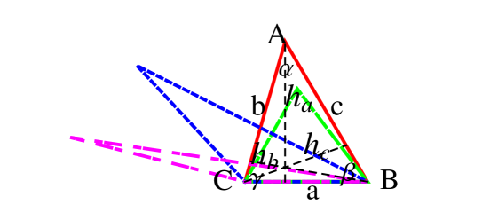
Figure 1: The triangle’s four distinct cases ${\cal A}$, ${\cal B}$, ${\cal C}$ and ${\cal D}$. Red continuous sides $\to$ shape ${\cal A}$, green dashed sides $\to$ shape ${\cal B}$, blue short-dashed sides $\to$ shape ${\cal C}$ and magenta dot-dashed sides $\to$ shape ${\cal D}$. The side lengths of the shown ${\cal A}$, ${\cal B}$, ${\cal C}$ and ${\cal D}$ triangles are (1, 1.5, 1.611), (1, 1.06, 1.127), (1, 1.5, 2.239) and (1, 1.5, 2.470), respectively.

Their names respectively are:

$${\cal A}\ \to \ \ h_{c}\ <\ h_{b}\ <\ a\ <\ h_{a}\ <\ b\ <\ c,\quad\gamma\,<\,{\pi}/{2}$$ (8)

$${\cal B}\ \to \ \ h_{c}\ <\ h_{b}\ <\ h_{a}\ <\ a\ <\ b\ <\ c,\quad\gamma\,<\,{\pi}/{2}$$

$${\cal C}\ \to \ \ h_{c}\ <\ h_{b}\ <\ a\ <\ h_{a}\ <\ b\ <\ c,\quad\gamma\,>\,{\pi}/{2}$$

$${\cal D}\ \to \ \ h_{c}\ <\ h_{b}\ <\ h_{a}\ <\ a\ <\ b\ <\ c,\quad\gamma\,>\,{\pi}/{2}.$$

These inequalities show that we have six $r$-intervals. In case ${\cal A}$ they are: $[0,\,h_{c}]$, $[h_{c},\,h_{b}]$, $[h_{b},\,a]$, $[a,\,h_{a}]$, $[h_{a},\,b]$ and $[b,\,c]$. They will be referred to as $I{\cal A},\,II{\cal A},\,III{\cal A},\,IV{\cal A},\,V{\cal A}$ and $VI{\cal A}$, respectively. The same convention is adopted in cases ${\cal B},\,{\cal C}$ and ${\cal D}$. Since intervals $I{\cal A}$, $I{\cal B}$, $I{\cal C}$ and $I{\cal D}$ coincide we shall simply speak of interval I. The same happens for intervals II and VI. In each of the subcases listed in Eq.(8) we can apply the procedure expounded in ref.[11] and determine the expression of the second derivative of the (isotropic) CF of the considered triangle. The procedure is straightforward though somewhat cumbersome. After putting

$${\cal A}(\alpha,\beta,\gamma)\equiv 3+(\pi-\alpha)\cot\alpha+(\pi-\beta)\cot\beta+(\pi-\gamma)\cot\gamma,$$ (9)

$${\cal B}(\alpha,\beta,\gamma)\equiv(\pi-2\alpha)\cot\alpha+(\pi-2\beta)\cot\beta+2(1+\gamma\cot\gamma),$$ (10)

$${\cal C}(\alpha,\beta,\gamma)\equiv 4+2(\pi-2\alpha)\cot\alpha+\pi\cot\beta+\pi\cot\gamma,$$ (11)

$$c(\alpha,\beta)\equiv\cot\alpha\,+\,\cot\beta$$ (12)

and

$$\Omega_{2}(x)\equiv-2x\sqrt{1-x^{2}}-2\arccos(x),$$ (13)

the final expressions of $\gamma^{{}^{\prime\prime}}(r)$ are

$${\gamma^{{}^{\prime\prime}}}_{{}_{I}}(r) = {{\cal A}(\alpha,\beta,\gamma)}/({2\pi S}),\quad\quad\quad\quad\quad\quad\quad\quad\quad\quad 0<r<h_{c};$$ (14)

$${\gamma^{{}^{\prime\prime}}}_{{}_{II}}(r) = [{c(\alpha,\beta)\Omega_{2}(h_{c}/r)+{\cal A}(\alpha,\beta,\gamma)}]/({2\pi S}),\quad\quad h_{c}<r<h_{b};$$ (15)

$${\gamma^{{}^{\prime\prime}}}_{{}_{III{\cal A}}}(r) = \frac{c(\alpha,\beta)\Omega_{2}(h_{c}/r)+c(\alpha,\gamma)\Omega_{2}(h_{b}/r)+{\cal A}(\alpha,\beta,\gamma)}{2\pi S},\,h_{b}<r<a;$$ (16)

$${\gamma^{{}^{\prime\prime}}}_{{}_{IV{\cal A}}}(r) = \frac{c(\alpha,\beta)\Omega_{2}(h_{c}/r)+c(\alpha,\gamma)\Omega_{2}(h_{b}/r)+{\cal C}(\alpha,\beta,\gamma)}{4\pi S},\,a<r<h_{a};$$ (17)

$${\gamma^{{}^{\prime\prime}}}_{{}_{V{\cal A}}}(r) = \bigl{[}c(\alpha,\beta)\Omega_{2}(h_{c}/r)+2c(\beta,\gamma)\Omega_{2}(h_{a}/r)+c(\alpha,\gamma)\Omega_{2}(h_{b}/r)$$ (18)

$$\quad\quad\quad\quad+{\cal C}(\alpha,\beta,\gamma)\bigr{]}/({4\pi S}),\quad\quad\quad\quad\quad\quad h_{a}<r<b;$$

$${\gamma^{{}^{\prime\prime}}}_{{}_{III{\cal B}}}(r) = {\gamma^{{}^{\prime\prime}}}_{{}_{III{\cal A}}}(r),\quad\quad\quad\quad\quad\quad\quad\quad\quad\quad\quad\quad\quad h_{b}<r<h_{a};$$ (19)

$${\gamma^{{}^{\prime\prime}}}_{{}_{IV{\cal B}}}(r) = \bigl{[}c(\alpha,\beta)\Omega_{2}(h_{c}/r)+c(\beta,\gamma)\Omega_{2}(h_{a}/r)+c(\alpha,\gamma)\Omega_{2}(h_{b}/r)$$ (20)

$$\quad\quad\quad\quad\quad+{\cal A}(\alpha,\beta,\gamma)\bigr{]}/{2\pi S},\quad\quad\quad\quad\quad\quad\quad h_{a}<r<a;$$

$${\gamma^{{}^{\prime\prime}}}_{{}_{V{\cal B}}}(r) = {\gamma^{{}^{\prime\prime}}}_{{}_{V{\cal A}}}(r),\quad\quad\quad\quad\quad\quad\quad\quad\quad\quad\quad\quad\quad a<r<b;$$ (21)

$${\gamma^{{}^{\prime\prime}}}_{{}_{III{\cal C}}}(r) = {\gamma^{{}^{\prime\prime}}}_{{}_{II}}(r),\quad\quad\quad\quad\quad\quad\quad\quad\quad\quad\quad\quad\ \ h_{b}<r<a;$$ (22)

$${\gamma^{{}^{\prime\prime}}}_{{}_{IV{\cal C}}}(r) = {\gamma^{{}^{\prime\prime}}}_{{}_{IV{\cal A}}}(r),\quad\quad\quad\quad\quad\quad\quad\quad\quad\quad\quad\quad a<r<h_{a};$$ (23)

$${\gamma^{{}^{\prime\prime}}}_{{}_{V{\cal C}}}(r) = {\gamma^{{}^{\prime\prime}}}_{{}_{IV{\cal C}}}(r),\quad\quad\quad\quad\quad\quad\quad\quad\quad\quad\quad\quad h_{a}<r<b;$$ (24)

$${\gamma^{{}^{\prime\prime}}}_{{}_{III{\cal D}}}(r) = {\gamma^{{}^{\prime\prime}}}_{{}_{III{\cal C}}}(r),\quad\quad\quad\quad\quad\quad\quad\quad\quad\quad\quad\quad\quad h_{b}<r<h_{a};$$ (25)

$${\gamma^{{}^{\prime\prime}}}_{{}_{IV{\cal D}}}(r) = {\gamma^{{}^{\prime\prime}}}_{{}_{II}}(r),\quad\quad\quad\quad\quad\quad\quad\quad\quad\quad\quad\quad\quad h_{a}<r<a;$$ (26)

$${\gamma^{{}^{\prime\prime}}}_{{}_{V{\cal D}}}(r) = {\gamma^{{}^{\prime\prime}}}_{{}_{IV{\cal A}}}(r),\quad\quad\quad\quad\quad\quad\quad\quad\quad\quad\quad\quad\quad a<r<b;$$ (27)

$${\gamma^{{}^{\prime\prime}}}_{{}_{VI}}(r) = \frac{c(\alpha,\gamma)\Omega_{2}(h_{b}/r)+c(\beta,\gamma)\Omega_{2}(h_{a}/r)+{\cal B}(\alpha,\beta,\gamma)}{4\pi S},\ b<r<c.$$ (28)

From these expressions the calculation of $\gamma^{{}^{\prime}}(r)$ is straightforward after noting that the primitive of $\Omega_{2}(h/x)$ is function $\Omega_{1}(h,x)$ reported below

$$\Omega_{1}(h,x)\equiv\frac{2h\sqrt{x^{2}-h^{2}}}{x}-2x\arccos(h/x).$$ (29)

In fact, integrating Eq. (28) over the interval $[r,\,c]$ with $b<r<c$ one finds that

$${\gamma^{{}^{\prime}}}_{{}_{VI}}(r) = \bigl{[}{\cal B}(\alpha,\beta,\gamma)(r-c)+c(\alpha,\gamma)(\Omega_{1}(h_{b},r)-\Omega_{1}(h_{b},c))+$$

$$\ c(\beta,\gamma)(\Omega_{1}(h_{a},r)-\Omega_{1}(h_{a},c))\bigr{]}/{4\pi S},\quad b<r<c,$$

where we used the property that $\gamma^{{}^{\prime}}(r)$ is continuous at $r=c$ and therefore equal to zero there. It is now convenient to put

$$\hat{\Omega}_{1}(h_{a},r,b)\equiv\Omega_{1}(h_{a},r)-\Omega_{1}(h_{a},b).$$ (30)

The previous derivative expression then reads

$${\gamma^{{}^{\prime}}}_{{}_{VI}}(r) = \bigl{[}{\cal B}(\alpha,\beta,\gamma)(r-c)+c(\alpha,\gamma)\hat{\Omega}_{1}(h_{b},r,c)+c(\beta,\gamma)\times$$

$$\quad\hat{\Omega}_{1}(h_{a},r,c)\bigr{]}/({4\pi S}),\quad\quad b<r<c,$$ (31)

In the same way, integrating Eq. (18) over the interval $[r,\,b]$ with $h_{a}<r<b$ and imposing the continuity at $r=b$, one finds that

$${\gamma^{{}^{\prime}}}_{{}_{V{\cal A}}}(r) = \frac{1}{4\pi S}\bigl{[}2c(\beta,\gamma)\hat{\Omega}_{1}(h_{a},r,b)+c(\alpha,\gamma)\hat{\Omega}_{1}(h_{b},r,b)+$$ (32)

$$\quad c(\alpha,\beta)\hat{\Omega}_{1}(h_{c},r,b)+{\cal C}(\alpha,\beta,\gamma)(r-b)\bigr{]}+{\gamma^{{}^{\prime}}}_{{}_{VI}}(b),\quad h_{a}<r<b,$$

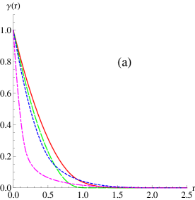
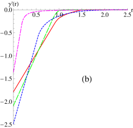
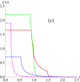
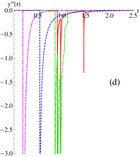
Figure 2: (a): plots of $\gamma(r)$ for triangle ${\cal A}$ (continuous red curve), ${\cal B}$ (green dashed curve), ${\cal C}$ (blue short-dashed) and ${\cal D}$ (magenta dot-dashed). The convention in the curve drawing is the same of Fig. 1; (b): plots of $\gamma^{{}^{\prime}}(r)$ (note, however, that $\gamma^{{}^{\prime}}(r)$ is scaled by a factor $1/5$ in case ${\cal D}$); (c): plots of $\gamma^{{}^{\prime\prime}}(r)$ (the shown $\gamma^{{}^{\prime\prime}}(r)$s are scaled by factors $1/5$ and $1/15$ in cases ${\cal C}$ and ${\cal D}$, respectively); (d): plots of $\gamma^{{}^{\prime\prime\prime}}(r)$ (the shown $\gamma^{{}^{\prime\prime\prime}}(r)$s are scaled by factors $1/20$, $1/5$, $1/10$ and $1/20$ in cases A, B, C and D).

and then, step by step, that

$${\gamma^{{}^{\prime}}}_{{}_{IV{\cal A}}}(r) = \frac{1}{4\pi S}\bigl{[}c(\alpha,\gamma)\hat{\Omega}_{1}(h_{b},r,h_{a})+c(\alpha,\beta)\hat{\Omega}_{1}(h_{c},r,h_{a})+$$ (33)

$$\quad{\cal C}(\alpha,\beta,\gamma)(r-h_{a})\bigr{]}+{\gamma^{{}^{\prime}}}_{{}_{V{\cal A}}}(h_{a}),\quad a<r<h_{a};$$

$${\gamma^{{}^{\prime}}}_{{}_{III{\cal A}}}(r) = \frac{1}{2\pi S}\bigl{[}c(\alpha,\gamma)\hat{\Omega}_{1}(h_{b},r,a)+c(\alpha,\beta)\hat{\Omega}_{1}(h_{c},r,a)+$$

$$\quad{\cal A}(\alpha,\beta,\gamma)(r-a)\bigr{]}+{\gamma^{{}^{\prime}}}_{{}_{IV{\cal A}}}(a),\quad\quad\quad h_{b}<r<a;$$ (34)

$${\gamma^{{}^{\prime}}}_{{}_{II{\cal A}}}(r) = \frac{c(\alpha,\beta)\hat{\Omega}_{1}(h_{c},r,b)+{\cal A}(\alpha,\beta,\gamma)(r-h_{b})}{2\pi S}+$$ (35)

$$\quad{\gamma^{{}^{\prime}}}_{{}_{III{\cal A}}}(h_{b}),\quad\quad\quad\quad\quad\quad h_{c}<r<h_{b};$$

$${\gamma^{{}^{\prime}}}_{{}_{I{\cal A}}}(r) = \frac{{\cal A}(\alpha,\beta,\gamma)(r-h_{c})}{2\pi S}+{\gamma^{{}^{\prime}}}_{{}_{II{\cal A}}}(h_{c}),\quad\quad 0<r<h_{c}.$$ (36)

The expressions of $\gamma^{{}^{\prime}}(r)$ are similarly obtained in the other three cases and are reported in the appendix. In the same way, from the resulting expressions of the first derivative, using the fact that a primitive of $(\Omega_{1}(h,x)$ is

$$\Omega(h,x)\equiv-{\pi x^{2}}/{2}+3h\sqrt{x^{2}-h^{2}}+(x^{2}+2h^{2})\arcsin(h/x),$$ (37)

starting from the outermost $r$-interval and imposing the continuity at the outermost end points one obtains the algebraic expression of the CF of a generic triangle. For instance, the CF expression in the outermost interval is

$${\gamma}_{{}_{VI}}(r) = \Bigl{[}{\cal B}(\alpha,\beta,\gamma)(r-c)^{2}/2+c(\alpha,\gamma)[\Omega(h_{b},r)-\Omega(h_{b},c)-\Omega_{1}(h_{b},c)\times$$

$$(r-c)]+c(\beta,\gamma)[\Omega(h_{a},r)-\Omega(h_{a},c)-\Omega_{1}(h_{a},c)(r-c))]\Bigr{]}/{4\pi S}.\ \quad\quad$$ (38)

This expression, after putting

$$\hat{\Omega}(h_{a},r,b)\equiv\Omega(h_{a},r)-\Omega(h_{a},b)-\Omega_{1}(h_{a},b)(r-b),$$ (39)

simplifies into

$${\gamma}_{{}_{VI}}(r) = [{\cal B}(\alpha,\beta,\gamma)(r-c)^{2}/2+c(\alpha,\gamma)\hat{\Omega}(h_{b},r,c)+$$ (40)

$$c(\beta,\gamma)\hat{\Omega}(h_{a},r,c)]/({4\pi S}),\quad\quad\quad b<r<c.$$

In the remaining interval, for case ${\cal A}$ one finds

$${\gamma}_{{}_{V{\cal A}}}(r) = \frac{1}{4\pi S}\Bigl{[}\frac{{\cal C}(\alpha,\beta,\gamma)(r-b)^{2}}{2}+c(\alpha,\beta)\hat{\Omega}(h_{c},r,b)+c(\alpha,\gamma)\hat{\Omega}(h_{b},r,b)+\quad\quad$$ (41)

$$\ 2c(\beta,\gamma)\hat{\Omega}(h_{a},r,b)\Bigr{]}+{\gamma^{{}^{\prime}}}_{{}_{VI}}(b)(r-b)+{\gamma}_{{}_{VI}}(b),\quad\quad h_{a}<r<b,$$

$${\gamma}_{{}_{IV{\cal A}}}(r) = \frac{1}{4\pi S}\Bigl{[}\frac{{\cal C}(\alpha,\beta,\gamma)(r-h_{a})^{2}}{2}+c(\alpha,\gamma)\hat{\Omega}(h_{b},r,h_{a})+c(\alpha,\beta)\times$$ (42)

$$\hat{\Omega}(h_{c},r,h_{a})\Bigr{]}+{\gamma^{{}^{\prime}}}_{{}_{V{\cal A}}}(h_{a})(r-h_{a})+{\gamma}_{{}_{V{\cal A}}}(h_{a}),\quad\quad\quad a<r<h_{a},$$

$${\gamma}_{{}_{III{\cal A}}}(r) = \frac{1}{4\pi S}\Bigl{[}\frac{{\cal A}(\alpha,\beta,\gamma)(r-a)^{2}}{2}+c(\alpha,\gamma)\hat{\Omega}(h_{b},r,a)+c(\alpha,\beta)\hat{\Omega}(h_{c},r,a)\Bigr{]}$$ (43)

$$\quad+{\gamma^{{}^{\prime}}}_{{}_{IV{\cal A}}}(a)(r-a)+{\gamma}_{{}_{IV{\cal A}}}(a),\quad\quad\quad\quad\quad\quad\quad\quad h_{b}<r<a,$$

$${\gamma}_{{}_{II{\cal A}}}(r) = \frac{1}{2\pi S}\Bigl{[}{\frac{{\cal C}(\alpha,\beta,\gamma)(r-h_{b})^{2}}{2}+c(\alpha,\beta)\hat{\Omega}(h_{c},r,h_{b})}\Bigr{]}+$$ (44)

$$\quad\quad{\gamma^{{}^{\prime}}}_{{}_{III{\cal A}}}(h_{b})(r-h_{b})+{\gamma}_{{}_{III{\cal A}}}(h_{b}),\quad\quad\quad\quad\quad\quad\quad h_{c}<r<h_{b},$$

$${\gamma}_{{}_{I{\cal A}}}(r) = \frac{{\cal A}(\alpha,\beta,\gamma)(r-h_{c})^{2}}{4\pi S}+{\gamma^{{}^{\prime}}}_{{}_{II{\cal A}}}(h_{c})(r-h_{c})+{\gamma}_{{}_{II{\cal A}}}(h_{c}),\ 0<r<h_{c}.$$ (45)

The expressions relevant to the other cases are given in the appendix. Figures 2a-d show the plots of $\gamma(r)$ and its first three derivatives for the four triangle cases. The CFs look each other rather similar because the different supports cannot be appreciated on the figure scale. The first derivatives show greater difference since their behaviours about $r=0$ signal that the specific length (i.e. the ratio perimeter/surface, see Eq.(4)) increases as one passes from case ${\cal A}$ to ${\cal D}$ (note that the magenta curve is scaled). The differences become more evident for the second derivatives and dramatic for the third one. Here the cuspids signal algebraic singularities $\propto(r-h)^{-1/2}$ and they involve the only heights which meet the opposite side within the triangle. This explains why Fig. 3d shows three spikes in cases ${\cal A}$ and ${\cal B}$ and only one spike in cases ${\cal C}$ and ${\cal D}$.

3 Conclusions

We have briefly described the cases where the algebraic knowledge of the CF of a plane figure can usefully be applied to analyze observed scattering intensities. In particular we have reported here the explicit expression of the CF of a general triangle. Besides their intrinsic interest for the shown singularities, which are important from the point of view of the figure reconstruction, these expressions allow us to evaluate the CF of the associated cylinder by a simple quadrature.

Appendix A Expressions for cases ${\cal B}$, ${\cal C}$ and ${\cal D}$

For completeness we give the expressions of the CF and its 1st derivative in remaining cases ${\cal B}$, ${\cal C}$ and ${\cal D}$. For the first derivative one finds

$$\gamma^{{}^{\prime}}_{{}_{VI{\cal B}}}(r) = \gamma^{{}^{\prime}}_{{}_{VI}}(r),\quad\quad\quad\quad\quad\quad\quad\quad\quad\quad\quad\quad\quad b<r<c;\quad\quad\quad\quad\quad\quad\quad\quad\quad\quad$$ (46)

$$\gamma^{{}^{\prime}}_{{}_{V{\cal B}}}(r) = \frac{1}{4\pi S}\Bigl{[}2{c}(\beta,\gamma)\hat{\Omega}_{1}(h_{a},r,b)+{c}(\alpha,\gamma)\hat{\Omega}_{1}(h_{b},r,b)+{c}(\alpha,\beta)\times$$ (47)

$$\hat{\Omega}_{1}(h_{c},r,b)+(r-b){{\cal C}}(\alpha,\beta,\gamma)\Bigr{]}+\gamma^{{}^{\prime}}_{{}_{VI}}(b),\quad\quad\quad\quad\quad a<r<b;$$

$$\gamma^{{}^{\prime}}_{{}_{IV{\cal B}}}(r) = \frac{1}{2\pi S}\Bigl{[}c(\alpha,\beta)\hat{\Omega}_{1}(h_{c},r,a)+c(\beta,\gamma)\hat{\Omega}_{1}(h_{a},r,a)+c(\alpha,\gamma)$$ (48)

$$\quad\hat{\Omega}_{1}(h_{b},r,a)+{\cal A}(\alpha,\beta,\gamma)(r-a)\Bigr{]}+\gamma^{{}^{\prime}}_{{}_{V{\cal B}}}(a),\quad\quad h_{a}<r<a;$$

$$\gamma^{{}^{\prime}}_{{}_{III{\cal B}}}(r) = \frac{1}{2\pi S}\Bigl{[}c(\alpha,\beta)\hat{\Omega}_{1}(h_{c},r,h_{a})+c(\alpha,\gamma)\hat{\Omega}_{1}(h_{b},r,h_{a})+$$ (49)

$$\quad{{\cal A}}(\alpha,\beta,\gamma)(r-h_{a})\Bigr{]}+\gamma^{{}^{\prime}}_{{}_{IV{\cal B}}}(h_{a}),\ \quad\quad\quad\quad\quad\quad\quad h_{b}<r<h_{a};$$

$$\gamma^{{}^{\prime}}_{{}_{II{\cal B}}}(r) = \frac{c(\alpha,\beta)\left(\Omega_{1}(h_{c},r)-\Omega_{1}(h_{c},h_{b})\right)+{\cal A}(\alpha,\beta,\gamma)(r-h_{b})}{2\pi S}$$ (50)

$$\quad\quad+\gamma^{{}^{\prime}}_{{}_{II{\cal B}}}(h_{b}),\quad\quad\quad\quad\quad\quad\quad\quad\quad\quad\quad\quad h_{c}<r<h_{b};$$

$$\gamma^{{}^{\prime}}_{{}_{I{\cal B}}}(r) = \frac{{\cal A}(\alpha,\beta,\gamma)(r-h_{c})}{2\pi S}+\gamma^{{}^{\prime}}_{{}_{II{\cal B}}}(h_{c}),\quad\quad\quad\quad\quad\quad 0<r<h_{c};$$ (51)

in case ${\cal B}$,

$$\gamma^{{}^{\prime}}_{{}_{VI{\cal C}}}(r) = \gamma^{{}^{\prime}}_{{}_{VI}}(r),\quad\quad\quad\quad\quad\quad\quad\quad\quad\quad\quad\quad\quad\quad\quad\quad\quad b<r<c;\quad\quad\quad\quad\quad\quad\quad\quad$$ (52)

$$\gamma^{{}^{\prime}}_{{}_{V{\cal C}}}(r) = \frac{1}{4\pi S}\bigl{[}c(\alpha,\gamma)\hat{\Omega}_{1}(h_{b},r,b)+c(\alpha,\beta)\hat{\Omega}_{1}(h_{c},r,b)+{\cal C}(\alpha,\beta,\gamma)(r-b)\bigr{]}$$ (53)

$$\quad\quad+\gamma^{{}^{\prime}}_{{}_{VI{\cal C}}}(b),\quad\quad\quad\quad\quad\quad\quad\quad\quad\quad\quad\quad h_{a}<r<b;$$

$$\gamma^{{}^{\prime}}_{{}_{IV{\cal C}}}(r) = \frac{1}{4\pi S}\bigl{[}c(\alpha,\gamma)\hat{\Omega}_{1}(h_{b},r,h_{a})+c(\alpha,\beta)\hat{\Omega}_{1}(h_{c},r,h_{a})+$$ (54)

$$\quad{\cal C}(\alpha,\beta,\gamma)(r-h_{a})\bigr{]}+\gamma^{{}^{\prime}}_{{}_{V{\cal C}}}(h_{a}),\quad\quad\quad\quad\quad\quad a<r<h_{a};$$

$$\gamma^{{}^{\prime}}_{{}_{III{\cal C}}}(r) = \frac{c(\alpha,\beta)\hat{\Omega}_{1}(h_{c},r,a)+{\cal A}(\alpha,\beta,\gamma)(r-a)}{2\pi S}+\gamma^{{}^{\prime}}_{{}_{IV{\cal C}}}(a),\quad h_{b}<r<a;$$ (55)

$$\gamma^{{}^{\prime}}_{{}_{II{\cal C}}}(r) = \frac{c(\alpha,\beta)\hat{\Omega}_{1}(h_{c},r,h_{b})+{\cal A}(\alpha,\beta,\gamma)(r-h_{b})}{2\pi S}+\gamma^{{}^{\prime}}_{{}_{II{\cal C}}}(h_{b}),\ \ h_{c}<r<h_{b};$$ (56)

$$\gamma^{{}^{\prime}}_{{}_{I{\cal C}}}(r) = \frac{{\cal A}(\alpha,\beta,\gamma)(r-h_{c})}{2\pi S}+\gamma^{{}^{\prime}}_{{}_{II{\cal C}}}(h_{c}),\quad\quad\quad\quad\quad\quad\quad\quad\quad 0<r<h_{c};$$ (57)

in case ${\cal C}$, and

$$\gamma^{{}^{\prime}}_{{}_{VI{\cal D}}}(r) = \gamma^{{}^{\prime}}_{{}_{VI}}(r),\quad\quad\quad\quad\quad\quad\quad\quad\quad\quad\quad\quad\quad\quad\quad\quad\quad b<r<c;\quad\quad\quad\quad$$ (58)

$$\gamma^{{}^{\prime}}_{{}_{V{\cal D}}}(r) = \frac{1}{4\pi S}\bigl{[}c(\alpha,\gamma)\hat{\Omega}_{1}(h_{b},r,b)+c(\alpha,\beta)\hat{\Omega}_{1}(h_{c},r,b)+$$ (59)

$$\quad{\cal C}(\alpha,\beta,\gamma)(r-b)\bigr{]}+\gamma^{{}^{\prime}}_{{}_{VI{\cal D}}}(a),\quad\quad\quad\quad\quad\quad\quad\quad\quad a<r<b;\quad\quad$$

$$\gamma^{{}^{\prime}}_{{}_{IV{\cal D}}}(r) = \frac{{\cal A}(\alpha,\beta,\gamma)(r-a)+c(\alpha,\beta)\hat{\Omega}_{1}(h_{c},r,a)}{2\pi S}+\gamma^{{}^{\prime}}_{{}_{V{\cal D}}}(a),\quad h_{a}<r<a;\quad\quad$$ (60)

$$\gamma^{{}^{\prime}}_{{}_{III{\cal D}}}(r) = \frac{{\cal A}\left(\alpha,\beta,\gamma\right)(r-h_{a})+c(\alpha,\beta)+\hat{\Omega}_{1}(h_{c},r,h_{b})}{2\pi S}+$$ (61)

$$\quad\gamma^{{}^{\prime}}_{{}_{IV{\cal D}}}(h_{a}),\quad\quad\quad\quad\quad\quad\quad\quad\quad\quad\quad\quad\quad\quad\quad h_{b}<r<h_{a};\quad$$

$$\gamma^{{}^{\prime}}_{{}_{II{\cal D}}}(r) = \frac{c(\alpha,\beta)\hat{\Omega}_{1}(h_{c},r,h_{b})+{\cal A}(\alpha,\beta,\gamma)(r-h_{b})}{2\pi S}+\gamma^{{}^{\prime}}_{{}_{II{\cal D}}}(h_{b}),\ h_{c}<r<h_{b};\quad\quad$$ (62)

$$\gamma^{{}^{\prime}}_{{}_{I{\cal D}}}(r) = \frac{{\cal A}(\alpha,\beta,\gamma)(r-h_{c})}{2\pi S}+\gamma^{{}^{\prime}}_{{}_{II{\cal D}}}(h_{c}),\quad\quad\quad\quad\quad\quad\quad\quad\ 0<r<h_{c}$$ (63)

in case ${\cal D}$.

For the CF one finds

$$\gamma_{{}_{VI{\cal B}}}(r) = \gamma_{{}_{VI}}(r),\quad\quad\quad b<r<c$$ (64)

$$\gamma_{{}_{V{\cal B}}}(r) = \frac{1}{4\pi S}\Bigl{[}2{c}(\beta,\gamma)\hat{\Omega}(h_{a},r,b)+{c}(\alpha,\gamma)\hat{\Omega}(h_{b},r,b)+{c}(\alpha,\beta)\hat{\Omega}(h_{c},r,b)$$ (65)

$$\quad\quad+{{\cal C}}(\alpha,\beta,\gamma)\frac{(r-b)^{2}}{2}\Bigr{]}+\gamma^{{}^{\prime}}_{{}_{VI}}(b)(r-b)+\gamma_{{}_{VI}}(b),\quad\quad a<r<b;$$

$$\gamma_{{}_{IV{\cal B}}}(r) = \frac{1}{2\pi S}\Bigl{[}{c}(\beta,\gamma)\hat{\Omega}(h_{a},r,a)+{c}(\alpha,\gamma)\hat{\Omega}(h_{b},r,a)+{c}(\alpha,\beta)\hat{\Omega}(h_{c},r,a)$$ (66)

$$\quad+{{\cal A}}(\alpha,\beta,\gamma)\frac{(r-a)^{2}}{2}\Bigr{]}+\gamma^{{}^{\prime}}_{{}_{V{\cal B}}}(a)(r-a)+\gamma_{{}_{V{\cal B}}}(a),\quad\quad h_{a}<r<a;$$

$$\gamma_{{}_{III{\cal B}}}(r) = \frac{1}{2\pi S}\Bigl{[}{c}(\alpha,\beta)\hat{\Omega}(h_{c},r,h_{a})+{c}(\alpha,\gamma)\hat{\Omega}(h_{b},r,h_{a})+{{\cal A}}(\alpha,\beta,\gamma)\frac{(r-h_{a})^{2}}{2}\Bigr{]}$$ (67)

$$\quad\quad+\gamma^{{}^{\prime}}_{{}_{IV{\cal B}}}(h_{a})(r-h_{a})+\gamma_{{}_{IV{\cal B}}}(h_{a}),\quad\quad\quad\quad\quad\quad\quad h_{b}<r<h_{a};$$

$$\gamma_{{}_{II{\cal B}}}(r) = \frac{1}{2\pi S}\Bigl{[}{c}(\alpha,\beta)\hat{\Omega}(h_{c},r,h_{b})+{{\cal A}}(\alpha,\beta,\gamma)\frac{(r-h_{b})^{2}}{2}\Bigr{]}$$ (68)

$$\quad\quad+\gamma^{{}^{\prime}}_{{}_{III{\cal B}}}(h_{b})(r-h_{b})+\gamma_{{}_{III{\cal B}}}(h_{b}),\quad\quad\quad\quad\quad\quad\quad h_{c}<r<h_{b};\quad\quad\quad\quad$$

$$\gamma_{{}_{I{\cal B}}}(r) = \frac{{{\cal A}}(\alpha,\beta,\gamma){(r-h_{c})^{2}}}{4\pi S}+\gamma^{{}^{\prime}}_{{}_{II{\cal B}}}(h_{c})(r-h_{c})+\gamma_{{}_{II{\cal B}}}(h_{c}),\quad 0<r<h_{c}\quad$$ (69)

in case ${\cal B}$,

$$\gamma_{{}_{VI{\cal C}}}(r) = \gamma_{{}_{VI}}(r),\quad\quad\quad\quad\quad\quad\quad\quad\quad\quad\quad\quad\quad\quad\quad\quad\quad\quad\quad\quad\quad b<r<c;\quad\quad\quad\quad$$ (70)

$$\gamma_{{}_{V{\cal C}}}(r) = \frac{1}{4\pi S}\Bigl{[}{c}(\alpha,\beta)\hat{\Omega}(h_{c},r,b)+{c}(\alpha,\gamma)\hat{\Omega}(h_{b},r,b)+{{\cal C}}(\alpha,\beta,\gamma){(r-b)^{2}}/{2}\Bigr{]}$$ (71)

$$\quad\quad+\gamma^{{}^{\prime}}_{{}_{VI}}(b)(r-b)+\gamma_{{}_{VI}}(b),\quad\quad\quad\quad\quad\quad\quad\quad h_{a}<r<b;$$

$$\gamma_{{}_{IV{\cal C}}}(r) = \frac{1}{4\pi S}\Bigl{[}{c}(\alpha,\beta)\hat{\Omega}(h_{c},r,h_{a})+{c}(\alpha,\gamma)\hat{\Omega}(h_{b},r,h_{a})+{{\cal C}}(\alpha,\beta,\gamma){(r-h_{a})^{2}}/{2}\Bigr{]}$$ (72)

$$\quad\quad+\gamma^{{}^{\prime}}_{{}_{V{\cal C}}}(h_{a})(r-h_{a})+\gamma_{{}_{V{\cal C}}}(h_{a}),\quad\quad\quad\quad\quad\quad\quad\quad a<r<h_{a};$$

$$\gamma_{{}_{III{\cal C}}}(r) = \frac{1}{2\pi S}\Bigl{[}{c}(\alpha,\beta)\hat{\Omega}(h_{c},r,a)+{{\cal A}}(\alpha,\beta,\gamma)\frac{(r-a)^{2}}{2}\Bigr{]}$$ (73)

$$\quad\quad+\gamma^{{}^{\prime}}_{{}_{IV{\cal C}}}(a)(r-a)+\gamma_{{}_{IV{\cal C}}}(a),\quad\quad\quad\quad\quad\quad\quad\quad h_{b}<r<a;$$

$$\gamma_{{}_{II{\cal C}}}(r) = \frac{1}{2\pi S}\Bigl{[}{c}(\alpha,\beta)\hat{\Omega}(h_{c},r,h_{b})+{{\cal A}}(\alpha,\beta,\gamma)\frac{(r-h_{b})^{2}}{2}\Bigr{]}$$ (74)

$$\quad\quad+\gamma^{{}^{\prime}}_{{}_{III{\cal C}}}(h_{b})(r-h_{b})+\gamma_{{}_{III{\cal C}}}(h_{b}),\quad\quad\quad\quad\quad\quad h_{c}<r<h_{b};$$

$$\gamma_{{}_{I{\cal C}}}(r) = \frac{{{\cal A}}(\alpha,\beta,\gamma){(r-h_{c})^{2}}}{4\pi S}+\gamma^{{}^{\prime}}_{{}_{II{\cal C}}}(h_{c})(r-h_{c})+\gamma_{{}_{II{\cal C}}}(h_{c}),\quad\quad 0<r<h_{c}$$ (75)

in case ${\cal C}$, and

$$\gamma_{{}_{VI{\cal D}}}(r) = \gamma_{{}_{VI}}(r),\quad\quad\quad\quad\quad\quad\quad\quad\quad\quad\quad\quad\quad\quad\quad\quad\quad\quad\quad\quad b<r<c;\quad\quad\quad\quad\quad\quad$$ (76)

$$\gamma_{{}_{V{\cal D}}}(r) = \frac{1}{4\pi S}\Bigl{[}{c}(\alpha,\beta)\hat{\Omega}(h_{c},r,b)+{c}(\alpha,\gamma)\hat{\Omega}(h_{b},r,b)+{{\cal C}}(\alpha,\beta,\gamma)\frac{(r-b)^{2}}{2}\Bigr{]}$$ (77)

$$\quad\quad+\gamma^{{}^{\prime}}_{{}_{VI}}(b)(r-b)+\gamma_{{}_{VI}}(b),\quad\quad\quad\quad\quad\quad\quad\quad\quad\quad a<r<b;$$

$$\gamma_{{}_{IV{\cal D}}}(r) = \frac{1}{2\pi S}\Bigl{[}{c}(\alpha,\beta)\hat{\Omega}(h_{c},r,a)+{{\cal A}}(\alpha,\beta,\gamma)\frac{(r-a)^{2}}{2}\Bigr{]}$$ (78)

$$\quad\quad+\gamma^{{}^{\prime}}_{{}_{V{\cal D}}}(a)(r-a)+\gamma_{{}_{V{\cal D}}}(a),\quad\quad\quad\quad\quad\quad\quad\quad\quad\quad h_{a}<r<a;$$

$$\gamma_{{}_{III{\cal D}}}(r) = \frac{1}{2\pi S}\Bigl{[}{c}(\alpha,\beta)\hat{\Omega}(h_{c},r,h_{a})+{{\cal A}}(\alpha,\beta,\gamma)\frac{(r-h_{a})^{2}}{2}\Bigr{]}$$ (79)

$$\quad\quad+\gamma^{{}^{\prime}}_{{}_{IV{\cal D}}}(h_{a})(r-h_{a})+\gamma_{{}_{IV{\cal D}}}(h_{a}),\quad\quad\quad\quad\quad\quad\quad\quad h_{b}<r<h_{a};$$

$$\gamma_{{}_{II{\cal D}}}(r) = \frac{1}{2\pi S}\Bigl{[}{c}(\alpha,\beta)\hat{\Omega}(h_{c},r,h_{b})+{{\cal A}}(\alpha,\beta,\gamma)\frac{(r-h_{b})^{2}}{2}\Bigr{]}$$ (80)

$$\quad\quad+\gamma^{{}^{\prime}}_{{}_{III{\cal D}}}(h_{b})(r-h_{b})+\gamma_{{}_{III{\cal D}}}(h_{b}),\quad\quad\quad\quad\quad\quad\quad\quad h_{c}<r<h_{b};$$

$$\gamma_{{}_{I{\cal D}}}(r) = \frac{{{\cal A}}(\alpha,\beta,\gamma){(r-h_{c})^{2}}}{4\pi S}+\gamma^{{}^{\prime}}_{{}_{II{\cal D}}}(h_{c})(r-h_{c})+\gamma_{{}_{II{\cal D}}}(h_{c}),\quad\quad 0<r<h_{c}$$ (81)

in case ${\cal D}$.


Acknowledgments

I thank Dr Wilfried Gille for his critical reading of the manuscript and for having checked most of the above formulae.

References

- [1] Guinier A and Fournét G 1955 Small-Angle Scattering of X-rays (New York: John Wiley)
- [2] Debye P, Anderson HR and Brumberger H 1957 J Appl Phys 20 518
- [3] Pedersen JS, Vyskocil P, Schönfeld B and Kostorz G 1997 J Appl Cryst 30 975
- [4] Goodisman J 1980 J Appl Cryst 13 132
- [5] Gille W 1987 Exp Tech Phys 35 93
- [6] Ciccariello S 1991 J Appl Cryst 24 509
- [7] Burger C and Ruland W 2001 Acta Cryst A 57 482
- [8] Ciccariello S 2005 J Appl Cryst A38 97
- [9] Gille W 2002 Powder Technology 123 292
- [10] Ciccariello S 2003 Acta Cryst A59 506
- [11] Ciccariello S 2009 J Math Phys 50 103527
- [12] Sulanke R 1961 Math Nach 23 51
- [13] Harutyunyan HS 2007 Scientific Letters of the Yerevan State University 1 17
- [14] Aharonyan NG and Ohanyan VK 2005 J of Contemporary Mathematical Analysis (Armenian Academy of Sciences) 40 43
- [15] Harutyunyan HS and Ohanyan VK 2009 Adv Appl Prob 41 358
- [16] Gille W, Aharonyan NG and Ohanyan VK 2009 J Appl Cryst 42 326
- [17] Burger C, Hsiao BS and Chu B 2010 Polymer Reviews 50 91
- [18] Sinha SK, Sirota EB, Garoff S and Stanley HB 1988 Phys Rev B 38 2297
- [19] Rauscher M, Salditt T and Spohn H 1995 Phys Rev B 52 16855
- [20] Lazzari R 2002 J Appl Cryst 35 406