Interferometric distillation and determination of unknown two-qubit entanglement

Abstract

We propose a scheme for both distilling and quantifying entanglement, applicable to individual copies of an arbitrary unknown two-qubit state. It is realized in a usual two-qubit interferometry with local filtering. Proper filtering operation for the maximal distillation of the state is achieved, by erasing single-qubit interference, and then the concurrence of the state is determined directly from the visibilities of two-qubit interference. We compare the scheme with full state tomography.

Introduction.— Multiparticle interference is a striking phenomenon connecting with quantum entanglement. For pure states, the connection is rather straightforward. In a two-particle interferometry Ghosh ; Horne , the interference visibility gives the concurrence Bennet_conc ; Wootters_conc , a widely used entanglement measure, of the two-particle pure state Jakob . In a multiparticle Aharonov-Bohm interferometry Sim , the visibility can be used to prove the quantum nonlocality of Greenberger-Horne-Zeilinger entanglement Greenberger . For mixed states, however, multiparticle interference comes from a mixture of entanglement and classical correlation, and it is hard to distinguish the two different correlations. It is interesting to find a way to extract entanglement from the interference, which is the aim of this work.

In quantum information research, there are strong demands of distilling and quantifying entanglement Horodecki_rev . Currently available schemes are of two types, one using multiple copies of a target state and the other using individual copies. Since the multiple copies are harder to prepare in laboratory in general, it may be necessary to explore further the latter type. The distillation of the latter type has been done using local filtering, for a known two-qubit state Kwiat or after full state tomography Wang . And no scheme of the latter type has been proposed for directly quantifying an entanglement measure, such as concurrence, of an arbitrary mixed state in experiments; note that the existing schemes of the former type for determining concurrence have not been realized Horodecki_copy or provide a lower bound of concurrence Mintert_mixed2 for mixed states, while concurrence was recently determined in experiments by using two copies of a pure state Walborn . Therefore, it is valuable to find a scheme of the latter type for distilling and directly determining entanglement of an unknown state (without full state reconstruction).

In this work, we propose an interferometric scheme for both distilling and determining entanglement, applicable to individual copies of an arbitrary unknown two-qubit state. It can be realized in a two-qubit interferometry with local filtering Kwiat ; Wang . The maximal distillation (the normal form Verstraete_filter ) of the state is first achieved, by iteratively erasing single-qubit interference, and then the concurrences of both the initial and the distilled states are directly determined from the visibilities of two-qubit interference. This quantification is based on our important findings that the two-qubit interference shows three different “local” extrema (visibilities) in general and that when the single-qubit interference is fully erased, the three extrema give the Lorentz singular values Verstraete_filter , a linear combination of which gives the concurrences. Our scheme is conceptually different from full state tomography and practically useful.

Figure 1: Two-qubit interferometry with local filtering. It consists of a source, distillation parts, and detection parts. The source generates individual copies of an arbitrary unknown state of two qubits A and B, each represented by pseudospins $\uparrow_{j}$ and $\downarrow_{j}$, $j=\mathrm{A},\mathrm{B}$. Qubit $\mathrm{A}$ flies to the detectors ($\mathrm{D}_{\mathrm{A}}$) of Alice, passing through three beam splitters (BS), while $\mathrm{B}$ to Bob ($\mathrm{D}_{\mathrm{B}}$); see solid arrows. The state is transformed into its maximally distilled state in the distillation parts, and then its concurrence is determined by measuring the visibilities of two-qubit interference in the detection parts.

Two-qubit interferometry with local filtering.— We introduce the interferometry (Fig. 1). The source generates individual copies of a state of two qubits A and B, which fly to Alice and Bob, respectively. The qubit degree of freedom, the pseudospin, can be photon polarization, particle path, particle spin, etc. For illustration, we choose particle path as the pseudospin, by considering two particles A and B, each injected to either the upper (pseudospin up) or the lower path (down) of its side.

The $4\times 4$ density matrix $\hat{\rho}$ of the initial two-qubit state is represented by using pseudospin basis states, and written by using a real matrix R as Schlienz

$$\hat{\rho}=\frac{1}{4}\sum_{l,l^{\prime}=0,1,2,3}R_{ll^{\prime}}\hat{\sigma}_{l}\otimes\hat{\sigma}_{l^{\prime}},\,\,\,\,\,R_{ll^{\prime}}\equiv\mathrm{Tr}(\hat{\rho}\hat{\sigma}_{l}\otimes\hat{\sigma}_{l^{\prime}}),$$ (1)

where $\mathrm{Tr}(\cdots)$ means the trace of matrix, $\hat{\sigma}_{0}$ is the $2\times 2$ identity matrix, and $\hat{\sigma}_{l}$’s ($l=1,2,3$) are the Pauli matrices. Then the single-qubit states ($\hat{\rho}_{j}\equiv\mathrm{Tr}_{\bar{j}}\hat{\rho}$) of Alice and Bob are represented by 4-vectors $(R_{00},R_{10},R_{20},R_{30})$ and $(R_{00},R_{01},R_{02},R_{03})$, respectively; $\mathrm{Tr}_{\bar{j}}(\cdots)$ means the trace over the degrees of freedom of qubit $\bar{j}$ $(\neq j)$.

In the distillation parts, which are absent in usual interferometries Ghosh ; Horne , Alice (Bob) has local operation $\hat{D}_{j}(f_{j},\theta_{\textrm{dis},j},\phi_{\textrm{dis},j})\equiv\hat{F}(f_{j})\hat{U}(\theta_{\textrm{dis},j},\phi_{\textrm{dis},j})$ on qubit $j=\mathrm{A}$ ($\mathrm{B}$). It transforms the initial state $\hat{\rho}$ into its normal form Verstraete_filter ; Verstraete_normal $\hat{\rho}_{\rm dis}$, its maximally distilled state Kent ,

$$\hat{\rho}_{\mathrm{dis}}=(\hat{D}_{\mathrm{A}}\otimes\hat{D}_{\mathrm{B}})\hat{\rho}(\hat{D}_{\mathrm{A}}\otimes\hat{D}_{\mathrm{B}})^{\dagger}.$$ (2)

The local filtering $\hat{F}(f_{j})$ and the rotation $\hat{U}(\theta_{\textrm{dis},j},\phi_{\textrm{dis},j})$ of qubit $j$ are supported by two beam splitters, $\mathrm{BS}_{2j}$ and $\mathrm{BS}_{1j}$, respectively, and represented as

$$\hat{F}(f)=\begin{pmatrix}1&0\\ 0&f\\ \end{pmatrix},\,\,\,\hat{U}(\theta,\phi)=\begin{pmatrix}\cos\frac{\theta}{2}&\sin\frac{\theta}{2}e^{-i\phi}\\ -\sin\frac{\theta}{2}e^{i\phi}&\cos\frac{\theta}{2}\\ \end{pmatrix}.$$ (3)

Here, $0\leq f_{j}\leq 1$ is the filtering parameter controlled by the reflection amplitude of $\mathrm{BS}_{2j}$, $\theta_{\textrm{dis},j}\in[0,\pi]$ parameterizes the transmission at $\mathrm{BS}_{1j}$, and $\phi_{\textrm{dis},j}\in[0,2\pi]$ is the phase shift. In the filtering operation $\hat{F}(f_{j})$, particle $j$ is abandoned with probability $1-f_{j}^{2}$ when it flies along the lower path after scattering by $\mathrm{BS}_{1j}$. Whether qubit $j$ is filtered off or not is certified at detector $\mathrm{D}_{3j}$. The two beam splitters constitute the minimal setup for the distillation. This is understood from the fact Verstraete_filter that each local operation on qubit $j$ corresponds to a Lorentz transformation of the 4-vector of qubit $j$. $\hat{F}$ and $\hat{U}$ correspond to the Lorentz boost and the spatial rotation, respectively. We emphasize that the Lorentz boost mathematically introduced in Ref. Verstraete_filter is physically realized here by $\hat{F}$, using beam splitter $\mathrm{BS}_{2j}$. We will see later how $\hat{D}_{j}$ is efficiently found for an unknown state $\hat{\rho}$.

In the detection parts, Alice and Bob count the number $n_{ij}$ of the particles $j$ arriving at detector $\mathrm{D}_{ij}$, $i=1,2$, during measurement time, long enough to get the statistical average of coincidence correlation $\langle n_{i\mathrm{A}}n_{i^{\prime}\mathrm{B}}\rangle$ for a given setting of all the beam splitters. They tune $\mathrm{BS}_{3\mathrm{A}}$ and $\mathrm{BS}_{3\mathrm{B}}$ to see single- and two-qubit interferences in $\langle n_{1j}(n_{1\bar{j}}+n_{2\bar{j}})\rangle$ and $\langle\delta n_{1\mathrm{A}}\delta n_{1\mathrm{B}}\rangle\equiv\langle n_{1\mathrm{A}}n_{1\mathrm{B}}\rangle-\langle n_{1\mathrm{A}}(n_{1\mathrm{B}}+n_{2\mathrm{B}})\rangle\langle n_{1\mathrm{B}}(n_{1\mathrm{A}}+n_{2\mathrm{A}})\rangle$, respectively; the other correlations involving $\mathrm{D}_{2j}$ contain the same information. Here, the number $n_{ij}$ is normalized by the total number $N$ of states ending in neither $\mathrm{D}_{3\mathrm{A}}$ nor $\mathrm{D}_{3\mathrm{B}}$, and $\langle n_{ij}(n_{1\bar{j}}+n_{2\bar{j}})\rangle$ means the average number $n_{ij}$ of qubit $j$ in the events where the other qubit $\bar{j}$ $(\neq j)$ is not filtered (does not end in $\mathrm{D}_{3\bar{j}}$). The qubit rotation at $\mathrm{BS}_{3j}$ is represented by $\hat{U}(\theta_{\textrm{det},j},\phi_{\textrm{det},j})$, where $\theta_{\textrm{det},j}\in[0,\pi]$ and $\phi_{\textrm{det},j}\in[0,2\pi]$. Note that the phase accumulation of particle $j$ along its path is absorbed in the rotation angles $\phi_{{\rm dis},j}$ and $\phi_{{\rm det},j}$.

The visibilities of single- and two-qubit interferences are defined, respectively, as Jaeger

$$\begin{split}\mathcal{V}_{j=\mathrm{A},\mathrm{B}}&=W[\langle n_{1j}(n_{1\bar{j}}+n_{2\bar{j}})\rangle],\\ \mathcal{V}_{\mathrm{AB}}&=W[\langle\delta n_{1\mathrm{A}}\delta n_{1\mathrm{B}}\rangle+1/4],\end{split}$$ (4)

where $W[x]\equiv(\mathrm{max}[x]-\mathrm{min}[x])/(\mathrm{max}[x]+\mathrm{min}[x])$ and $\mathrm{max}[x]$ ($\mathrm{min}[x]$) means the local maxima (minima) of $x$ over the parameter space of $\mathrm{BS}_{3\mathrm{A}}$ and $\mathrm{BS}_{3\mathrm{B}}$, $\{\theta_{\textrm{det},\textrm{A}},\phi_{\textrm{det},\textrm{A}},\theta_{\textrm{det},\textrm{B}},\phi_{\textrm{det},\textrm{B}}\}$. Since the mean value of $\langle\delta n_{1\mathrm{A}}\delta n_{1\mathrm{B}}\rangle$ over the space is zero, the ad hoc factor $1/4$ is added in Eq. (4) so that the values of $\mathcal{V}_{\mathrm{AB}}$ are equal to the local maxima of $\langle\delta n_{1\mathrm{A}}\delta n_{1\mathrm{B}}\rangle$. Note that one needs to tune the transmission probability $\cos^{2}\frac{\theta_{\textrm{det},j}}{2}$ of $\mathrm{BS}_{3j}$, to obtain the information of the diagonal parts of $\hat{\rho}$ Jaeger .

Entanglement distillation.— We first explain how to transform $\hat{\rho}$ into $\hat{\rho}_{\mathrm{dis}}$. It is based on the facts Verstraete_normal that local density matrices $\hat{\rho}_{\mathrm{dis},j}\equiv\mathrm{Tr}_{\bar{j}}\hat{\rho}_{\textrm{dis}}$ of the normal form are proportional to the identity matrix and that any initial state $\hat{\rho}$ can be transformed iteratively to its normal form by filtering operations. In our interferometry, we find that these facts are realized as follows. When $\hat{\rho}_{\mathrm{dis}}$ is achieved in the distillation parts, the single-qubit interference visibilities $\mathcal{V}_{\mathrm{A}}$ and $\mathcal{V}_{\mathrm{B}}$ vanish, since the identity generates no interference. Thus, one can obtain $\hat{D}_{j}$ in an iterative way such that Alice and Bob alternately tune her/his beam splitters of the distillation parts to make the visibility $\mathcal{V}_{j}$ of her/his single-qubit interference vanish, until $\mathcal{V}_{\mathrm{A}}$ and $\mathcal{V}_{\mathrm{B}}$ both vanish simultaneously.

We describe each iteration step. In the $(2k-1)$-th step, $k=1,2,\cdots$, Alice observes the single-qubit interference signal in $\langle n_{1\mathrm{A}}(n_{1\mathrm{B}}+n_{2\mathrm{B}})\rangle$ by tuning $\mathrm{BS}_{3\mathrm{A}}$, with setting her parameters as $(f_{\mathrm{A}},\theta_{\mathrm{dis},\mathrm{A}})=(1,0)$ but without tuning $(f^{(2k-2)}_{\mathrm{B}},\theta^{(2k-2)}_{\mathrm{dis},\mathrm{B}},\phi^{(2k-2)}_{\mathrm{dis},\mathrm{B}})$ fixed by Bob; in the first step, Bob starts with $(f^{(0)}_{\mathrm{B}},\theta^{(0)}_{\mathrm{dis},\mathrm{B}})=(1,0)$. By comparing the signal with its general form, $\langle n_{1\mathrm{A}}(n_{1\mathrm{B}}+n_{2\mathrm{B}})\rangle=(1+\vec{\gamma}_{\mathrm{A}}\cdot\vec{v}_{\mathrm{A}})/2$, Alice determines $\vec{\gamma}_{\mathrm{A}}\equiv(\gamma_{\mathrm{A1}},\gamma_{\mathrm{A2}},\gamma_{\mathrm{A3}})$, which in fact represents the spatial part of the 4-vector of qubit $\mathrm{A}$; the general form has only a pair of extrema $\pm|\vec{\gamma}_{\mathrm{A}}|$, i.e., $\mathcal{V}_{\mathrm{A}}$ $(=|\vec{\gamma}_{\mathrm{A}}|)$ is single-valued. Here $\vec{v}_{j}\equiv(\sin\theta_{\mathrm{det},j}\cos\phi_{\mathrm{det},j},\sin\theta_{\mathrm{det},j}\sin\phi_{\mathrm{det},j},\cos\theta_{\mathrm{det},j})$ is the rotation vector of $\mathrm{BS}_{3j}$. Then, by setting $f_{\mathrm{A}}^{(2k-1)}=\sqrt{(1-|\vec{\gamma}_{\mathrm{A}}|)/(1+|\vec{\gamma}_{\mathrm{A}}|)}$ and the rotation vector of $\mathrm{BS}_{\mathrm{1A}}$ in the $(2k-1)$-th step as $\vec{v}_{\mathrm{dis,A}}^{(2k-1)}=-\vec{\gamma}_{\mathrm{A}}/|\vec{\gamma}_{\mathrm{A}}|$, Alice achieves the situation that $\mathcal{V}^{(2k-1)}_{\mathrm{A}}$ vanishes; after the setting, $\vec{\gamma}_{\mathrm{A}}$ rotates to be parallel to $\vec{z}=(0,0,-1)$ at $\mathrm{BS}_{\mathrm{1A}}$, and then vanishes by the filtering at $\mathrm{BS}_{\mathrm{2A}}$. Next, Bob performs his $(2k)$-th step in the same way as Alice’s $(2k-1)$-th step, except for the exchange $\mathrm{A}\leftrightarrow\mathrm{B}$. After such iterations, the distillation parameters converge to $(f_{j},\theta_{\mathrm{dis},j},\phi_{\mathrm{dis},j})$, at which $\mathcal{V}_{\mathrm{A}}=\mathcal{V}_{\mathrm{B}}=0$ and $\hat{\rho}_{\mathrm{dis}}$ is obtained.

Entanglement determination.— Before discussing entanglement quantification, we first show an interesting feature of $\mathcal{V}_{\mathrm{AB}}$. For a state $\hat{\rho}^{\prime}$, transformed from $\hat{\rho}$ by an arbitrary setting of the distillation parts, we derive a compact form of the cross-correlation, $\langle\delta n_{1\mathrm{A}}\delta n_{1\mathrm{B}}\rangle=\frac{1}{4}\vec{v}_{\mathrm{A}}\mathbf{Q}^{\prime}\vec{v}_{\mathrm{B}}^{T}$, where $\vec{v}_{j}$ is the rotation vector of $\mathrm{BS}_{3j}$, the column vector $\vec{v}^{T}_{\mathrm{B}}$ is the transpose of $\vec{v}_{\mathrm{B}}$, $\textbf{Q}^{\prime}$ is the $3\times 3$ matrix defined by $Q_{ll^{\prime}}^{\prime}=R^{\prime}_{ll^{\prime}}/R^{\prime}_{00}-R^{\prime}_{l0}R^{\prime}_{0l^{\prime}}/(R^{\prime}_{00})^{2}$, $l,l^{\prime}=1,2,3$, and $\textbf{R}^{\prime}$ is the real parametrization of $\hat{\rho}^{\prime}$ in Eq. (1); the number normalization by $N$ gives the factors $1/R^{\prime}_{00}$ and $1/(R^{\prime}_{00})^{2}$ in $Q_{ll^{\prime}}^{\prime}$. From this compact form and the fact that $\vec{v}_{j=\mathrm{A},\mathrm{B}}$ spans over the surface of unit sphere, it is easy to see that $\langle\delta n_{1\mathrm{A}}\delta n_{1\mathrm{B}}\rangle$ has three pairs of “local” extrema $\pm\lambda_{l}$’s ($\lambda_{1}\geq\lambda_{2}\geq\lambda_{3}\geq 0$), i.e., $\mathcal{V}_{\mathrm{AB}}$ has the three values $\lambda_{l}$’s, and that $\lambda_{l}$’s are identical to the singular values of $\textbf{Q}^{\prime}$ up to sign factor. Here, $\lambda_{1}$ is the global maximum of $\langle\delta n_{1\mathrm{A}}\delta n_{1\mathrm{B}}\rangle$, while $\lambda_{2}$ ($\lambda_{3}$) is the maximum over the space of $\vec{v}_{\mathrm{A}}$ and $\vec{v}_{\mathrm{B}}$ orthogonal to $\vec{v}_{\mathrm{A},1}$ and $\vec{v}_{\mathrm{B},1}$ ($\vec{v}_{\mathrm{A},1}$, $\vec{v}_{\mathrm{B},1}$, $\vec{v}_{\mathrm{A},2}$, and $\vec{v}_{\mathrm{B},2}$), where $\vec{v}_{j,l}$ is the rotation vector of $\mathrm{BS}_{3j}$ at which $\langle\delta n_{1\mathrm{A}}\delta n_{1\mathrm{B}}\rangle$ shows $\lambda_{l}$.

The above finding becomes very useful when $\hat{\rho}_{\mathrm{dis}}$ is achieved in the distillation parts ($\hat{\rho}^{\prime}=\hat{\rho}_{\mathrm{dis}}$ and $\textbf{R}^{\prime}=\textbf{R}_{\mathrm{dis}}$). In this case, the visibilities $\lambda_{l}$’s give the Lorentz singular values Verstraete_normal of the initial state as

$$s_{0}=\frac{N}{Mf_{\mathrm{A}}f_{\mathrm{B}}},\,\,\,s_{1}=s_{0}\lambda_{1},\,\,\,s_{2}=s_{0}\lambda_{2},\,\,\,s_{3}=qs_{0}\lambda_{3},$$ (5)

since they are equal to the singular values of $\textbf{R}_{\mathrm{dis}}/(f_{\mathrm{A}}f_{\mathrm{B}})$, $R_{\mathrm{dis},l0}=R_{\mathrm{dis},0l}=0$, and $R_{\textrm{dis},00}=N/M$. Here, $M$ is the total number of injection of $\hat{\rho}$ from the source, $q=\mathrm{Det}(\vec{v}_{\mathrm{A},1},\vec{v}_{\mathrm{A},2},\vec{v}_{\mathrm{A},3})\mathrm{Det}(\vec{v}_{\mathrm{B},1},\vec{v}_{\mathrm{B},2},\vec{v}_{\mathrm{B},3})$ is the sign factor guaranteeing the correct singular value decomposition, $\mathrm{Det}(\cdots)$ means matrix determinant, and $(\vec{v}_{j,1},\vec{v}_{j,2},\vec{v}_{j,3})$ is the matrix whose columns are $\vec{v}_{j,l}$’s. Using the relation Verstraete_filter between concurrence and Lorentz singular values, we find an important result that the concurrences $\mathcal{C}$ of $\hat{\rho}$ and $\hat{\rho}_{\mathrm{dis}}$ are directly obtained from $\mathcal{V}_{\mathrm{AB}}$,

$$\begin{split}\mathcal{C}(\hat{\rho})&=s_{0}\mathcal{C}(\hat{\rho}_{\mathrm{dis}}),\\ \mathcal{C}(\hat{\rho}_{\mathrm{dis}})&=\mathrm{max}[0,\frac{1}{2}(-1+\lambda_{1}+\lambda_{2}-q\lambda_{3})].\end{split}$$ (6)

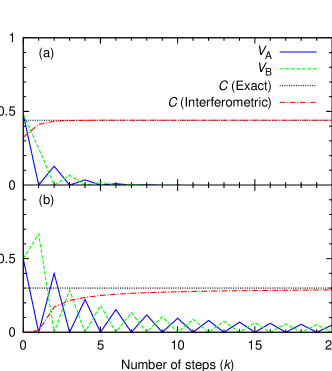
Figure 2: (Color online) The concurrence $\mathcal{C}^{(k)}(\hat{\rho})$ (dot-dashed lines), determined from the two-qubit visibilities $\mathcal{V}_{\mathrm{AB}}$, and the single-qubit visibilities $\mathcal{V}^{(k)}_{\mathrm{A}}$ and $\mathcal{V}^{(k)}_{\mathrm{B}}$ in the $k$-th distillation step are shown for (a) $\hat{\rho}_{\epsilon,\lambda}=\lambda|\phi_{\epsilon}\rangle\langle\phi_{\epsilon}|+\frac{1-\lambda}{2}(|\uparrow\downarrow\rangle\langle\uparrow\downarrow|+|\downarrow\uparrow\rangle\langle\downarrow\uparrow|)$ with $(\epsilon,\lambda)=(0.5,0.8)$ and (b) $\hat{\rho}=\frac{1}{2}|\uparrow\uparrow\rangle\langle\uparrow\uparrow|+\frac{2}{5}|\Psi_{+}\rangle\langle\Psi_{+}|+\frac{1}{10}|\Psi_{-}\rangle\langle\Psi_{-}|$, where $|\phi_{\epsilon}\rangle=(\epsilon|\uparrow\uparrow\rangle+|\downarrow\downarrow\rangle)/\sqrt{1+\epsilon^{2}}$ and $|\Psi_{\pm}\rangle=\frac{1}{\sqrt{2}}(|\downarrow\uparrow\rangle\pm|\uparrow\downarrow\rangle)$. The case (a) is typical, showing rapid convergence to $\hat{\rho}_{\mathrm{dis}}$, while (b) is an asymptotic case with slow convergence. For comparison, the exact value Wootters_conc of $\mathcal{C}(\hat{\rho})$ is given (dotted lines).

Examples.— In Fig. 2, the concurrence is determined at each $k$-th iteration step, for two examples of $\hat{\rho}$, using $\mathcal{V}_{\mathrm{AB}}$ and Eq. (6). For typical cases of $\hat{\rho}$ (non-asymptotic case) [Fig. 2(a)], $\mathcal{V}^{(k)}_{j=\mathrm{A,B}}$ vanishes rapidly within a few steps, and the determined value $\mathcal{C}^{(k)}(\hat{\rho})$ approaches to the exact value $\mathcal{C}(\hat{\rho})$ more rapidly. In this case, the deviation of $\mathcal{C}^{(k)}(\hat{\rho})$ from $\mathcal{C}(\hat{\rho})$ is estimated footnote as $|\mathcal{C}(\hat{\rho})-\mathcal{C}^{(k)}(\hat{\rho})|\propto(\mathcal{V}^{(k)}_{j})^{2}$ for small $\mathcal{V}^{(k)}_{j}$ ($\lesssim 0.1$). Thus, one can determine a precise value of $\mathcal{C}$ even before the complete distillation. The properties of particular types of $\hat{\rho}$ are given below.

(i) When $\hat{\rho}$ is pure, only one distillation step is necessary, since $\mathcal{V}^{(k)}_{\mathrm{A}}=\mathcal{V}^{(k)}_{\mathrm{B}}$ for all $k$ due to the complementarity Jakob . Note that $(\mathcal{V}^{(k=0)}_{j=\mathrm{A,B}})^{2}+\mathcal{C}^{2}(\hat{\rho})=1$ for $f_{\mathrm{A}}=f_{\mathrm{B}}=1$.

(ii) When $\hat{\rho}$ is separable and uncorrelated, $\hat{\rho}=\hat{\rho}_{\mathrm{A}}\otimes\hat{\rho}_{\mathrm{B}}$, the local properties of A and B are independent. Therefore, only two steps are required, $\mathcal{V}_{\mathrm{AB}}=0$, and $\mathcal{C}(\hat{\rho})=0$. Particularly, when either $\hat{\rho}_{\mathrm{A}}$ or $\hat{\rho}_{\mathrm{B}}$ is pure, its single-qubit visibility is one at $k=0$, and $\hat{\rho}$ cannot be distilled as $\hat{\rho}_{\mathrm{dis}}$ vanishes. When $\hat{\rho}$ is separable but has classical correlations, on the other hand, more than two steps are neccessary, $\mathcal{V}_{\mathrm{AB}}\neq 0$, and $\mathcal{C}(\hat{\rho})=0$.

(iii) When $\hat{\rho}$ is a Werner state or a Bell-diagonal state Bennet_conc ; Werner , the distillation is not necessary.

(iv) There is the so-called asymptotic case Verstraete_filter , where large number of steps are necessary [Fig. 2(b)] and most states are abandoned by the filtering ($f_{j}^{(k\to\infty)}\to 0$).

State	Distillation	Quantification	Total	Tomography
Bell	2400  (0)	$9\times 100+3\times 200$	3900	360
Werner	2400  (0)	$9\times 500+3\times 4000$	18900	38700
$\bf{I}/4$	2400  (0)	$9\times 100+3\times 7800$	26700	24300
$\hat{\rho}^{\prime}_{0.6}$	2400   (0)	$9\times 300+3\times 3800$	16500	30600
$\hat{\rho}_{0.9,0.6}$	7200  (1)	$9\times 500+3\times 6800$	32100	54900
$\hat{\rho}_{0.5,0.8}$	40800  (5)	$9\times 600+3\times 9600$	75000	38700

Table 1: Monte Carlo simulation Altepeter of the minimum number of individual copies of a given state $\hat{\rho}$, that need to be used to determine its concurrence [or $s_{0}(-1+\lambda_{1}+\lambda_{2}-q\lambda_{3})/2$ in Eq. (6)] within $\pm 0.01$ statistical error in our scheme (fourth column) and by full state tomography Tomography (fifth). In our scheme, it is the sum of the number of necessary copies for the distillation (second column) with $k_{\mathrm{dis}}$ iterative steps, and that for the quantification (third) consisting of nine measurement settings for the determination of $\vec{v}_{j,l}$ and three settings for the three maxima $\lambda_{l}$’s; the parentheses show $k_{\mathrm{dis}}$. In the distillation, the copies are used to achieve and to check $\mathcal{V}_{j}^{(k_{\mathrm{dis}})}<0.1$; for the tested states, this condition of $\mathcal{V}_{j}^{(k_{\mathrm{dis}})}$ is enough to obtain $\mathcal{C}$ within the $\pm 0.01$ error. On the other hand, among available tomography schemes, we consider here the most efficient one with nine measurement settings and four detectors. We test six representative states usually tested in entanglement detection Altepeter ; Kwiat , a Bell state $|\Psi_{0}\rangle=\frac{1}{\sqrt{2}}(|\uparrow\uparrow\rangle+|\downarrow\downarrow\rangle)$, a Werner state $\hat{\rho}_{W}=\frac{2}{3}{|\Psi_{0}\rangle\langle\Psi_{0}|}+\frac{1}{3}\frac{\bf{I}}{4}$, $\bf{I}/4$, $\hat{\rho}^{\prime}_{p}=|\Psi_{0}\rangle\langle\Psi_{0}|+\frac{p-1}{2}(|\uparrow\uparrow\rangle\langle\downarrow\downarrow|+|\downarrow\downarrow\rangle\langle\uparrow\uparrow|)$, and $\hat{\rho}_{\epsilon,\lambda}$ (introduced in Fig. 2) with two different sets of $(\epsilon,\lambda)$. Note that the efficiency of our scheme strongly depends on $\hat{\rho}$ (as the tomography) and becomes worse for states more filtered (those with smaller $N/M$); $N/M=1$ (no distillation; $k_{\mathrm{dis}}=0$) for the first four states, $0.95$ for $\hat{\rho}_{0.9,0.6}$, and $0.42$ for $\hat{\rho}_{0.5,0.8}$.

Below, we propose an optimal way of determining concurrence. After the distillation, one first determines all the rotation vectors $\vec{v}_{j,l}$, by observing $\langle\delta n_{1\mathrm{A}}\delta n_{1\mathrm{B}}\rangle$ in nine different settings of $\mathrm{BS}_{\mathrm{3A}}$ and $\mathrm{BS}_{\mathrm{3B}}$ and comparing the results with the compact form of $\langle\delta n_{1\mathrm{A}}\delta n_{1\mathrm{B}}\rangle$ (derived before). Then, one measures $\langle\delta n_{1\mathrm{A}}\delta n_{1\mathrm{B}}\rangle$ (thus $\lambda_{l}$) at the determined setting of $\mathrm{BS}_{3j=\mathrm{A(B)}}$ at $\vec{v}_{\mathrm{A(B)},l}$. We emphasize that a crude determination of $\vec{v}_{j,l}$ is enough for a precise detection of $\lambda_{l}$ and $\mathcal{C}$. It is because $\lambda_{l}$ is a local maximum, around which a small error ($\sim\delta$) in the direction $\vec{v}_{j,l}$ for $\lambda_{l}$ causes only a much smaller error ($\sim\delta^{2}$) in the value of $\lambda_{l}$. This makes our scheme efficient. Table I shows that for states not much filtered, our scheme is as efficient as the tomography Tomography for the quantification of the initial state. For the distillation and the quantification together, it can be more efficient than previous tomographic schemes, e.g., in Ref. Wang ; the previous schemes require roughly 2-4 times larger number of state copies than our scheme, as they require the tomography twice (once before and once after the distillation). Moreover, our scheme improves previous distillations Kwiat ; Wang , as it is applicable to unknown states. Therefore, our scheme is practically useful, in the situation Altepeter ; Enk that for unknown states, the existing schemes are less efficient than the tomography and virtually require it.

Conclusion.— We have proposed a “quantum entanglement concentrator”, in which the entanglement of an arbitrary unknown two-qubit state is distilled and determined. We remark the following meaningful features.

First, our scheme is within experimental reach and applicable to generic types of qubits, as it has only local operations using a tunable beam splitter, currently available Kwiat . Second, we show that even for mixed states, concurrence and Lorentz singular values are directly and experimentally accessible, interestingly from the extrema of two-qubit interference; concurrence has been determined experimentally only for a pure state Walborn . This motivates to study the features of the singular values Verstraete_Bell . Third, entanglement quantification can be closely related with distillation Kwiat ; Bennett ; Pan . In our scheme, the former can be done after the latter. Finally, our scheme may be practically useful (e.g., for teleportation Verstraete_tele ), as it achieves the distillation and the quantification within one framework. It would be valuable to generalize our scheme to larger systems of multiple qubits, where tomography error estimation becomes less feasible.

We thank J. B. Altepeter, N. Gisin, Hee Su Park, and Tzu-Chieh Wei for valuable discussions, and especially the group of P. G. Kwiat for the numerical code for the tomography. This work was supported by KAIST-HRHRP.

References

(1) R. Ghosh and L. Mandel,
Phys. Rev. Lett. 59, 1903 (1987).
(2) M. Horne, A. Shimony, and A. Zeilinger,
Nature 347, 429 (1990).
(3) C. H. Bennett, D. P. DiVincenzo, J. A. Smolin, and W. K. Wootters,
Phys. Rev. A 54, 3824 (1996).
(4) W. K. Wootters, Phys. Rev. Lett. 80,
2245 (1998).
(5) M. Jakob and J. A. Bergou,
arXiv:quant-ph/0302075v1 (2003).
(6) H.-S. Sim and E. V. Sukhorukov,
Phys. Rev. Lett. 96, 020407 (2006).
(7) D. M. Greenberger, M. A. Horne, A. Shimony, and A. Zeilinger,
Am. J. Phys. 58, 1131 (1990).
(8) R. Horodecki, P. Horodecki, M. Horodecki, and K. Horodecki,
arXiv:quant-ph/0702225v2 (2007).
(9) J. B. Altepeter et al.,
Phys. Rev. Lett. 95, 033601 (2005).
(10) P. G. Kwiat, S. Barraza-Lopez, A. Stefanov, and N. Gisin,
Nature 409, 1014 (2001).
(11) Z.-W. Wang et al.,
Phys. Rev. Lett. 96, 220505 (2006).
(12) P. Horodecki,
Phys. Rev. Lett. 90, 167901 (2003).
(13) F. Mintert and A. Buchleitner,
Phys. Rev. Lett. 98, 140505 (2007).
(14) S. P. Walborn et al.,
Nature 440, 1022 (2006).
(15) F. Verstraete, J. Dehaene, and B. DeMoor,
Phys. Rev. A 64, 010101(R) (2001).
(16) J. Schlienz and G. Mahler,
Phys. Rev. A 52, 4396 (1995).
(17) F. Verstraete, J. Dehaene, and B. De Moor,
Phys. Rev. A 68, 012103 (2003).
(18) A. Kent, N. Linden, and S. Massar,
Phys. Rev. Lett. 83, 2656 (1999).
(19) G. Jaeger, A. Shimony, and L. Vaidman,
Phys. Rev. A 51, 54 (1995).
(20) The details of the estimation will be
given elsewhere.
(21) R. F. Werner,
Phys. Rev. A 40, 4277 (1989).
(22)
We obtain the code for the tomography
from the group of P. G. Kwiat;
D. F. V. James, P. G. Kwiat, W. J. Munro, and A. G. White, Phys. Rev. A 64, 052312 (2001).
(23) S. J. van Enk, N. Lütkenhaus, and H. J. Kimble,
Phys. Rev. A 75, 052318 (2007).
(24) F. Verstraete and M. M. Wolf,
Phys. Rev. Lett. 89, 170401 (2002).
(25) C. H. Bennett et al.,
Phys. Rev. Lett. 76, 722 (1996).
(26) J.-W. Pan et al.,
Nature 423, 417 (2003).
(27) F. Verstraete and H. Verschelde,
Phys. Rev. Lett. 90, 097901 (2003).