Geometric phase with nonunitary evolution in presence of a quantum critical bath

Abstract

Geometric phases, arising from cyclic evolutions in a curved parameter space, appear in a wealth of physical settings. Recently, and largely motivated by the need of an experimentally realistic definition for quantum computing applications, the quantum geometric phase was generalized to open systems. The definition takes a kinematical approach, with an initial state that is evolved cyclically but coupled to an environment — leading to a correction of the geometric phase with respect to the uncoupled case. We obtain this correction by measuring the nonunitary evolution of the reduced density matrix of a spin one-half coupled to an environment. In particular, we consider a bath that can be tuned near a quantum phase transition, and demonstrate how the criticality information imprinted in the decoherence factor translates into the geometric phase. The experiments are done with a NMR quantum simulator, in which the critical environment is modeled using a one-qubit system.

For decades, the geometric phase berry (GP) has fascinated physicists for its elegant theoretical grounds and its practical applications anandan . The GP is resilient to dynamical perturbations, thus, it might serve as a naturally fault-tolerant quantum information processing device cirac . In order to explore such applications, and unlike traditional studies of the GP in closed systems with pure states, one must take into account realistic experimental conditions — i.e. the explicit presence of noise and environments. Uhlmann was the first in considering a system in a mixed state, embeded, as a subsystem, in a larger system that is in a pure state uhlmann . Later, Sjöqvist et al Sjoqvist put forward a definition of the GP for a general mixed state undergoing a cyclic unitary evolution — subsequently measured using NMR interferometry in Ref. Du . Different approaches to the problem were proposed openGP . In the present Letter, we will follow the line of Tong et al. tong06 , who developed a kinematic generalization of the GP to open systems that takes into account the coupling to an environment (leading to a nonunitary evolution of the reduced density matrix of the system LombardoVillar .) Arguably, this approach is better suited to explore the usefulness of the GP in a real quantum computer undergoing decoherence processes SjoqvistPhysics . Here we report a measurement of the GP for a spin $1/2$ undergoing nonunitary evolution induced by the coupling to an environment, using the decoherence factor or fidelity decay Quan . In particular —motivated by the recent observation that baths near quantum criticality induce strong decoherence Quan — we choose an environment that can be tuned near a quantum phase transition (QPT). This choice not only adds richness to the behavior of the GP, but also advances the program of understanding it in general open systems SjoqvistPhysics . In our experiments, performed in a NMR quantum simulator, we measure the full time dependence of the decoherence factor of the system-spin — from which we can determine the GP using the results of Ref. tong06 . For the environment, we introduce a simple qualitative model of the ground state degeneracy that occurs at QPTs. Apart from demonstrating an alternative to traditional interferometry-based approaches for measuring the GP in open systems, our results further establish the strong connections between quantum information, quantum criticality, decoherence, and the quantum geometric phase Quan ; GeometricTensor ; GPcritical ; carollo-pachos that have been the focus of much recent research (especially in the context of quantum simulations Jingfu ; JingfuFernando ).

The correction to the GP by a critical environment was first studied by Yi and Wang YiWang , who gave some general analytical results and found numerical instabilities in the GP of a qubit near criticallity of the bath (an $XY$ spin chain). More recently, it was shown that the GP of a spin coupled to an antiferromagnetic environment changes suddenly when the bath undergoes a first order QPT Yuang . Notice that our problem is seemingly related to, but different than, the use of the GP as an order parameter in a QPT of a closed system, as studied first by Carollo and Pachos and others carollo-pachos ; GPcritical .

We consider a spin $1/2$ coupled to an environment with a total Hamiltonian $H=\Omega Z_{\cal S}\otimes I_{\cal E}+Z_{\cal S}\otimes H_{\cal SE}+I_{\cal S}\otimes H_{\cal E}$, where $H_{\cal E}$ is the Hamiltonian of the bath, $Z_{\cal S}$ is the $z$ Pauli matrix of the system, $I_{\cal S}$ is the identity operator of the system and $I_{\cal E}$ the one of the bath. For simplicity, we only consider a dephasing spin–bath interaction, $Z_{\cal S}\otimes H_{\cal SE}$, neglecting relaxation effects and limiting the relevance of the initial state (see discussion below). We take a product initial state for the spin-bath system, $\rho(0)=\left|\psi_{0}\right>\left<\psi_{0}\right|\otimes\left|\varepsilon(0)\right>\left<\varepsilon(0)\right|$, where $\left|\psi_{0}\right>=\sin(\theta/2)\left|0\right>+\cos(\theta/2)\left|1\right>$ and $\left|\varepsilon(0)\right>$ is a general initial state of the bath. In absence of the bath, the spin follows an evolution around the Bloch sphere, reaching again the initial state for $\tau=2\pi/\Omega$. To compute the global phase gain during the evolution, one can use the Pancharatnam’s definition Pancharatnam , which contains a gauge dependent part (i.e a dynamical phase $\Phi_{d}=-\pi\cos(\theta)$) and a gauge independent part, commonly known as geometric phase $\Phi_{g}=\pi(1-\cos(\theta))$. When coupled to the bath, the reduced density matrix of the system at a time $t$ is

$$\rho_{\rm r}(t)=\sin^{2}(\theta/2)\left|0\right>\left<0\right|+\cos^{2}(\theta/2)\left|1\right>\left<1\right|$$

$$+\frac{\sin\theta}{2}e^{-i2\Omega t}r(t)\left|0\right>\left<1\right|+\frac{\sin\theta}{2}e^{i2\Omega t}r^{*}(t)\left|1\right>\left<0\right|.$$ (1)

Here, $r(t)=\left<\varepsilon_{0}(t)|\varepsilon_{1}(t)\right>$ is the decoherence factor induced by the environment, with $\left|\varepsilon_{k}(t)\right>=e^{-it\left[H_{B}+(-1)^{k}H_{\cal SE}\right]}\left|\varepsilon(0)\right>$. The phase $\Phi$ acquired by the open system after a period $\tau$ is defined as tong06 ,

$$\Phi=\arg\left[\sum_{k}\sqrt{\epsilon_{k}(\tau)\epsilon_{k}(0)}\left<k(0)|k(\tau)\right>e^{-\int_{0}^{\tau}dt\left<k(t)\right|\frac{\partial}{\partial t}\left|k(t)\right>}\right],$$ (2)

where $\left|k(t)\right>$ and $\epsilon_{k}(\tau)$ are respectively the instantaneous eigenvectors and eigenvalues of $\rho_{\rm r}(t)$. Of the two $k$ modes ($+$ and $-$) of the one qubit model we are treating, only the $+$ mode contributes to the GP. Because our environments can induce a complex decoherence factor, i.e. $r(t)=|r(t)|e^{-i\varphi}$, we obtain a slightly different expression than that shown in Ref. LombardoVillar , namely

$$\Phi =\int_{0}^{\tau}dt\left(\Omega-\frac{\partial\varphi}{\partial t}\right)\sin^{2}(\frac{\theta^{+}_{t}}{2})+$$ (3)

$$\tan^{-1} \frac{\sin\varphi(\tau)\sin(\frac{\theta^{+}_{\tau}}{2})\sin(\frac{\theta}{2})}{\cos\varphi(\tau)\sin(\frac{\theta^{+}_{\tau}}{2})\sin(\frac{\theta}{2})+\cos(\frac{\theta^{+}_{\tau}}{2})\cos(\frac{\theta}{2})},$$

where we have defined

$$\cos(\theta^{+}_{t}/2)=\frac{2(\epsilon_{+}-\sin^{2}(\theta/2))}{\sqrt{|r(t)|^{2}\sin^{2}(\theta)+4(\epsilon_{+}-\sin^{2}(\theta/2))^{2}}}$$ (4)

$$\sin(\theta^{+}_{t}/2)=\frac{|r(t)|\sin(\theta)}{\sqrt{|r(t)|^{2}\sin^{2}(\theta)+4(\epsilon_{+}-\sin^{2}(\theta/2))^{2}}}.$$ (5)

During normal quantum evolution, the system gains a global phase. The central result of Eq. (3) is to extract (by a proper choice of the “parallel transport condition”) the purification independent part of the phase — which can be termed a geometric phase because it is gauge invariant and reduces to the known results in the limit of a unitary evolution.

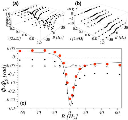
Figure 1: (a) Observed absolute value squared of the decoherence factor and (b) its argument, both as a function of time and external magnetic field strength. (c) Computed correction to the geometric phase for a choice of $\theta=\pi/4$. In large filled circles is the experimental data, and in solid line is the theoretically expected value (without free parameters). The corrected GP is the difference between the GP measured in presence of the environment (small filled circles), and the GP measured when the system and environment are decoupled (small empty circles). In this setup, $\Omega=100\pi\ {\rm Hz}$, $\Delta=0.02\Omega$, and $\delta=0.1\Omega$.

We have studied Eq. (3) both numerically and analytically with an Ising spin chain environment (see supplementary material EPAPS ), a paradigmatic example of a quantum phase transition. In particular, the non-analiticity of the GP at the critical point in the thermodynamical limit becomes evident in the limit of weak system-bath coupling EPAPS . Nevertheless, a full quantum simulation of a large enough critical system is on the edge of current technology, and beyond the scope of this Letter. Therefore, before turning to the experimental results, let us discuss briefly our choice for modeling a critical environment.

Near its critical point, the spectrum of a quantum critical system is characterized by the closing of the energy gap between the ground and the first excited state. In the thermodynamical limit, the gap closes with a power law $\sim|\lambda-\lambda_{c}|^{z\nu}$ (where $z$ and $\nu$ are critical exponents), but for all finite size systems there is a minimum gap $\Delta$ near $\lambda_{c}$. It is remarkable that, for many purposes, this feature of the spectrum is enough to describe qualitatively the effects of a critical environment: as long as the excitations involved are small, and one is only interested in qualitative behavior, a small energy expansion of the decoherence factor can justify considering just two levels with appropriate dynamics JingfuFernando . Thus, we propose to mimic a complex critical bath using a simple two-level system model with Hamiltonian $H_{\cal E}=\lambda\left|\lambda\right|^{z\nu-1}\Delta\ Z_{\cal E}+\Delta\ X_{\cal E}$, where $\lambda_{c}=0$ represents the “critical point” or QPT. The simplification might seem excessive, but it has been used successfully before: For $z\nu=1$ (the mean field exponents), it gives a correct qualitative description of the creation of topological excitations during a finite speed quench damski . In essence, the model is quantitatively not far away from the small systems used in demonstrations of quantum phase transitions ions ; Jingfu . A complete characterization of when this model does not describe the correct physics of a critical model is missing (one such example is the calculation of the path length of an adiabatic evolution somma ). Nevertheless, our results show that for the GP problem the model gives a fair description when the gap $\Delta$ is much smaller than the natural frequency $\Omega$ of the system spin.

Using a tomographic approach, we measure the GP of a qubit coupled to a critical environment using a nuclear magnetic resonance (NMR) quantum simulator, with the environment represented by the two level model described above (with critical exponents $z\nu=1$ and a dimensionless transverse field strength $B=\lambda\Delta$). The target Hamiltonian to simulate experimentally is: $H=\Omega Z_{\cal S}+\delta Z_{\cal S}Z_{\cal E}+BZ_{\cal E}+\Delta X_{\cal E}$, where $Z_{\cal S}$ and $Z_{\cal E}$ are the $z$ Pauli matrices of the system and environment respectively. We obtain the GP by measuring the magnetization of the system spin in the $X-Y$ plane, which gives us the decoherence factor $r(t)$.

Denoting by $\epsilon_{\pm}=\pm\Delta\sqrt{1+\lambda^{2z\nu}}$ the eigenenergies of $H_{\cal E}$, the decoherence factor of this model is

$$r(t) = e^{i\epsilon_{-}(\lambda)t}\left[\cos\epsilon_{-}(\lambda+\delta)t-\right.$$ (6)

$$i \left.\frac{\epsilon^{2}_{-}(\lambda+\delta)-\Delta^{2}\delta^{2}}{\epsilon_{-}(\lambda)\epsilon_{-}(\lambda+\delta)}\sin\epsilon_{-}(\lambda+\delta)t\right].$$

where, to simplify notation, we have chosen the system–environment interaction to be $H_{\cal SE}=\delta(I_{\cal S}-Z_{\cal S})Z_{\cal E}$. The correction to the GP due to this decoherence factor [shown in Fig. (1) with the experimental results to be discussed below] contains the main elements observed in more complex models, as Ising spin chains EPAPS : a maximum correction of the GP at criticality, and a small asymmetric correction far away from the critical point. From this simplified model we can get insight into the physics of true quantum critical baths.

Overall, the experimental sequence is as follows: We first fix $\Omega$, $\delta$, and $\Delta$. Then, for each value of $B$, we initialize the system, and measure the decoherence factor $r(t)$ of the system after evolution with an operator $U=e^{-iHt}$ for various times $t\in[0,2\pi/\Omega]$. The measured decoherence factor is shown in Fig. (1$a$) and (1$b$). The GP is calculated using a numerical interpolation of $r(t)$ in Eq. (3).

We choose the C¹³ and H¹ spins in the molecule of carbon-13 labelled chloroform (CHCl₃) dissolved in d6-acetone as the quantum registers (qubits) for the demonstration. The C¹³ atom simulates the system, and the H¹ the environment, where the scalar coupling between them is measured to be $J=215$ Hz. Data were taken with a Bruker DRX 700 MHz spectrometer.

Our choice of system–environment coupling makes the decoherence factor $r(t)$ independent of the initial state of the system (given by the angle $\theta$) [see Eq. (1)]. This, in turn, makes the GP depend trivially on $\theta$, which can be fully appreciated when approximating Eq. (3) in the weak coupling regime (see supplementary material EPAPS ). Because we concentrate on how the criticality properties of the bath affect the GP, it is experimentally convenient to fix an initial state of the system that maximizes the signal to noise ratio, and change only the parameters of the environment spin. In particular, we choose the input state of the system to be $(|0\rangle_{\cal S}+|1\rangle_{\cal S})/\sqrt{2}$. The corresponding decoherence factor can then be used to compute Eq. (3) for any other initial state of the system. From Eq. (1) we can see that $r(t)$ is encoded in the coherent terms proportional to $\langle 2\sigma_{+}\rangle$ [see Fig. (2$b$)], which can be observed directly in NMR by adding the two complex amplitudes of the peaks in the $C^{13}$ spectra.

We use the gate sequence of Fig. (2-a) pure1 ; pure2 ; pure3 to prepare the pseudo-pure state $|00\rangle_{\cal SE}$, to which we apply the unitary $e^{-i\pi Y_{\cal S}/4}e^{i\alpha Y_{\cal E}/2}$ to reach the input state $|\psi_{in}\rangle=(|0\rangle+|1\rangle)_{\cal S}|g\rangle_{\cal E}/\sqrt{2}$. Here $|g\rangle_{\cal E}$ is the ground state of the environment for a given $B$-value, $|g\rangle_{\cal E}=|0\rangle\cos(\alpha/2)-|1\rangle\sin(\alpha/2)$, where $\tan\alpha=-\Delta/B$. Because the decoherence factor is independent of the initial state of the system, we chose it such that it maximizes the signal-to-noise ratio of the experiment.

The quantum simulated evolution $U$ for a time $t$ can be implemented with a Trotter approximation average1 ; average2 ,

$$U\approx e^{-i\Delta tX_{\cal E}/2}e^{-i\delta tZ_{\cal S}Z_{\cal E}}e^{-i\Omega tZ_{\cal S}}e^{-iBtZ_{\cal E}}e^{-i\Delta tX_{\cal E}/2}$$ (7)

where we choose $\Omega=100\pi\ {\rm Hz}$, $\Delta=0.02\Omega$, $\delta=0.1\Omega$, and we apply the evolution operator $\tau/t$ times. We checked numerically that the Trotter approximation reduces the fidelity less than $0.3\%$ for $B\in[-0.2\Omega,0.2\Omega]$. Furthermore, we decompose the unitary operations $e^{-iBtZ_{\cal E}}$ as $e^{-i\pi X_{\cal E}/4}e^{-iBtY_{\cal E}}e^{i\pi X_{\cal E}/4}$, and $e^{-i\Omega tZ_{\cal S}}$ as $e^{-i\pi X_{\cal S}/4}e^{-i\Omega tY_{\cal S}}e^{i\pi X_{\cal S}/4}$ so that we can implement them with standard rf pulses. The coupling operation $e^{-i\delta tZ_{\cal S}Z_{\cal E}}$ is realized using the natural spin coupling with an evolution time $2\delta t/(\pi J)$. After the evolution $U$, we measure the magnetization in the $XY$ plane, which is proportional to the decoherence factor $r(t)$. The whole gate sequence for each measurement is shown in Fig. (2-b). Notice that we measure the absolute value as well as the complex phase of $r(t)$, necessary for the GP. The total evolution time was always well below the natural decoherence time of the quantum simulator.

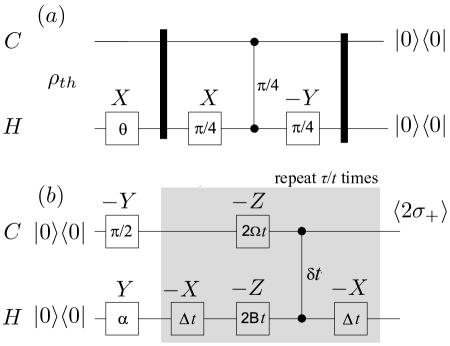
Figure 2: $(a)$ Gate sequence for preparing the pseudo-pure state $|00\rangle_{\cal SE}$ from the thermal state $\rho_{th}=\gamma_{C}Z_{\cal S}+\gamma_{H}Z_{\cal E}$, where $\gamma_{C}$ and $\gamma_{H}$ denote the gyromagnetic ratio of C¹³ and H¹. $(b)$ Gate sequence for the quantum simulation of the system and measurement of the decoherence factor $r(\tau)$, which is proportional to $\langle 2\sigma_{+}\rangle=\langle X+iY\rangle$. In both plots the rectangles denote single-qubit gates, implemented through radio-frequency pulses. The rotation angle is shown inside the rectangle, and the direction above. In the experiment we used $\cos\theta=2\gamma_{C}/\gamma_{H}\approx 1/2$ and $\tan\alpha=-\Delta/B$ with $\alpha\in(0,\pi)$. The narrow black rectangles denote the gradient pulses along $Z$-axis. The two filled circles connected by a line denote the $J-$ coupling evolution $e^{-i\phi Z_{\cal S}Z_{\cal E}}$, where $\phi$ is indicated next to the line.

To eliminate systematic errors, we repeat the experiment but uncoupling the system and the environment ($\delta=0$). From this we compute a baseline GP, which we subtract from the full (coupled) experiment. Thus, we obtain the correction to the GP due to the presence of the critical environment, which agrees well with theoretical expectations [see Fig. (1)$c$].

Conclusions. Using a NMR quantum simulator, we have obtained the quantum geometric phase of an open system undergoing nonunitary evolution. The geometric phase is computed in a tomographic manner, i.e. we measure the off-diagonal elements of the reduced density matrix of the system, from which we extract the decoherence factor that we use in the definition of the open system GP. In future work, we will introduce a third (probe) spin to perform an independent and direct measurement of the GP using traditional interferometry-based techniques Du . Our experiments support the observation that when the environment is near a second order quantum phase transition, the correction to the GP becomes singular. For our experiments, we introduced a simplified two-level model that captures the essence of the spectral behavior of the critical environment: the closing of the gap. By adding stochastic fields and further spins, we can quantum-simulate more realistic environments and couplings to the system, so that each initial state is affected differently by the bath. Despite the apparent simplicity of our experiment, we believe that the techniques we developed are quite general and applicable to more complex quantum simulations, and to related approaches such as bath engineering engbaths — designing an environment so that it induces a system to relax and decohere to interesting quantum many-body pure states.

We acknowledge helpful discussions with A. Acín, J. I. Cirac, P. Hauke, M. Lewenstein, G. Morigi, A. Roncaglia, and A. M. Souza. F.M.C. acknowledges financial support from Spanish MEC project TOQATA, ERC Advanced Grant QUAGATUA, and Caixa Manresa. F.C.L is supported by UBA, CONICET and ANPCyT–Argentina. P.I.V acknowledges financial support from the UNESCO LOREAL Women in Science Programme.

Appendix A Supplementary Material

In these supplementary notes we show how the open system geometric phase (GP) behaves in the limit of weak coupling to the environment. After analyzing the structure of the dominant terms, we will obtain analytically closed formulas for the case of an Ising spin chain environment, and compare to exact numerical results. The analytical results will show explicitly the singularity of the GP when the environment is at the critical point of a quantum phase transition.

A.0.1 Small coupling expansion of the geometric phase

The GP for an open system [Eq. (3) in the main text] is

$$\Phi =\int_{0}^{\tau}dt\left(\Omega-\frac{\partial\varphi}{\partial t}\right)\sin^{2}(\frac{\theta^{+}_{t}}{2})+$$ (8)

$$\tan^{-1} \frac{\sin\varphi(\tau)\sin(\frac{\theta^{+}_{\tau}}{2})\sin(\frac{\theta}{2})}{\cos\varphi(\tau)\sin(\frac{\theta^{+}_{\tau}}{2})\sin(\frac{\theta}{2})+\cos(\frac{\theta^{+}_{\tau}}{2})\cos(\frac{\theta}{2})},$$

where

$$\cos(\theta^{+}_{t}/2)=\frac{2(\epsilon_{+}-\sin^{2}(\theta/2))}{\sqrt{|r(t)|^{2}\sin^{2}(\theta)+4(\epsilon_{+}-\sin^{2}(\theta/2))^{2}}}$$ (9)

$$\sin(\theta^{+}_{t}/2)=\frac{|r(t)|\sin(\theta)}{\sqrt{|r(t)|^{2}\sin^{2}(\theta)+4(\epsilon_{+}-\sin^{2}(\theta/2))^{2}}},$$ (10)

and the only relevant eigenvalue of the reduced density matrix of the system is

$$\varepsilon_{+}=\frac{1}{2}\left(1+\sqrt{\cos^{2}(\theta)+|r|^{2}\sin^{2}(\theta)}\right).$$ (11)

We want to obtain a more tractable expression of the GP in the limit of small coupling between the system and the environment. For this, we expand the decoherence factor $r(t)=|r(t)|e^{i\varphi(t)}$ in powers of the system–environment coupling strength $\delta$,

$$|r(t)|^{2} = 1-R_{(2)}(t)\delta^{2}-R_{(3)}(t)\delta^{3}+{\cal O}(\delta^{4})$$ (12)

$$\varphi(t) = \varphi_{(1)}(t)\delta+\varphi_{(2)}(t)\delta^{2}+\varphi_{(3)}(t)\delta^{3}+{\cal O}(\delta^{4})$$

The zeroth order in $\varphi$ can be assimilated as an overall phase in the environment, and the first order in $|r(t)|^{2}$ is zero for environments with a finite spectral band width, as with spin environments app:CucchiettiPazZurek . At this level of approximation, the arc-tangent term in Eq. (8) can be expanded as

$$\sin^{2}\frac{\theta}{2}\left\{\varphi_{(1)}(\tau)\delta+\varphi_{(2)}(\tau)\delta^{2}+\left[\varphi_{(3)}(\tau)-\frac{1}{2}\cos\theta\cos^{2}\frac{\theta}{2}\varphi_{(1)}(\tau)\left(R_{(2)}(\tau)+\frac{\varphi^{2}_{(1)}(\tau)}{3}\right)\right]\right\},$$ (13)

while the term with the integral is

$$\pi (1-\cos\theta)-\sin^{2}\frac{\theta}{2}\varphi_{(1)}(\tau)\delta-\left[\sin^{2}\frac{\theta}{2}\varphi_{(2)}(\tau)+\frac{\Omega}{4}\cos\theta\sin^{2}\theta\left(\int_{0}^{\tau}dt\ R_{(2)}(t)\right)\right]\delta^{2}$$ (14)

$$- \left[\sin^{2}\frac{\theta}{2}\varphi_{(3)}(\tau)+\frac{1}{4}\cos\theta\sin^{2}\theta\left(\Omega\int_{0}^{\tau}dt\ R_{(3)}(t)-\int_{0}^{\tau}dt\ R_{(2)}(t)\frac{\partial\varphi_{(1)}}{\partial t}(t)\right)\right]\delta^{3},$$

where we have assumed that $\varphi_{(1)}(0)=\varphi_{(2)}(0)=\varphi_{(3)}(0)=0$. Adding up the two contributions results in

$$\Phi \simeq \pi(1-\cos\theta)-\cos\theta\sin^{2}\theta\left[\delta^{2}\frac{1}{4}\Omega\int_{0}^{\tau}R_{(2)}(t)\ dt\right.$$ (15)

$$+ \left.\frac{1}{24}\delta^{3}\left(3R_{(2)}(\tau)\varphi_{(1)}(\tau)+\varphi^{3}_{(1)}(\tau)+6\Omega\int_{0}^{\tau}R_{(3)}(t)\ dt-6\int_{0}^{\tau}R_{(2)}(t)\frac{\partial\varphi_{(1)}}{\partial t}(t)\ dt\right)\right].$$

A.0.2 GP from an Ising spin chain environment

Let us consider as the environment a paradigmatic example of quantum criticality: the Ising spin chain model with a homogeneous transverse field, with Hamiltonian

$$H_{\cal E}(\lambda)=-J\left(\sum_{n}Z_{n}Z_{n+1}+\lambda X_{n}\right),$$ (16)

where $N$ is the number of spins in the chain, $J$ the spin-spin coupling, $\lambda$ the dimensionless strength of the external field, and $X_{n}$ and $Z_{n}$ are the Pauli matrices of the n-th spin. The quantum critical point is at $\lambda_{c}=1$ app:pfeuty . If the system spin couples homogeneously to the Ising chain with strength $\delta$ (i.e. $H_{\cal SE}=\delta\sum_{n}Z_{n}$) this model can be solved analytically using a standard Jordan-Wigner transformation app:Quan into free fermionic modes. Notice that the requirement of homogeneous coupling is only for simplicity and can be relaxed in general app:Fazio . The decoherence factor induced by this environment —with the chain initially in the ground state of $H_{\cal E}$— decomposes into a product of factors, each coming independently from a different bath mode app:Quan ,

$$r(t)=\prod_{k>0}R_{k}(t)e^{i(\varphi_{k}(t)-\varepsilon_{k}t)}=Re^{i\varphi},$$ (17)

where $\varepsilon_{k}=2\sqrt{1+\lambda^{2}-2\lambda\cos(k)}$, with $k=\pm\frac{1}{2}\frac{2\pi}{N},\pm\frac{3}{2}\frac{2\pi}{N},...,\pm\frac{N-1}{2}\frac{2\pi}{N}$. This particular product form stems from the fact that the environment modes are non-interacting, each contributing and independent factor

$$R_{k}(t) = \sqrt{\cos^{2}\tilde{\varepsilon}_{k}t+\sin^{2}\tilde{\varepsilon}_{k}t\cos^{2}2\alpha_{k}},$$ (18)

$$\varphi_{k}(t) = -i\log\left(e^{i\varepsilon_{k}t}\sqrt{\frac{\cos\tilde{\varepsilon}_{k}t+i\sin\tilde{\varepsilon}_{k}t\cos 2\alpha_{k}}{\cos\tilde{\varepsilon}_{k}t-i\sin\tilde{\varepsilon}_{k}t\cos 2\alpha_{k}}}\right),$$

where $\tilde{\varepsilon}_{k}=2\sqrt{1+(\lambda+\delta)^{2}-2(\lambda+\delta)\cos(k)}$, $2\alpha_{k}=\left[\theta_{k}(\lambda+\delta)-\theta_{k}(\lambda)\right]$, and $\tan(\theta_{k})=\frac{\sin(2\pi k/N)}{\lambda-\cos(2\pi k/N)}.$

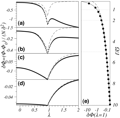
Figure 3: Correction $\delta\Phi=\Phi-\Phi_{0}$ to the geometric phase of a system spin in presence of an Ising chain environment (circles). In panels (a) through (d) we show the correction as a function of the strength $\lambda$ of the transverse field of the environment chain. The values of the self–energies of the system are $\Omega=1J,2J,5J,$ and $10J$, for panels (a), (b), (c), and (d) respectively. Here $J$ is the interaction strength between spins in the environment. In solid line is the third order approximation, and in dashed line the second order one. The phase correction is shown normalized by the length of the environment chain $N$ and the strength of the coupling to the environment squared, $\delta^{2}$. In all plots $N=100$ and $\delta=5\ 10^{-5}J$. In panel (e) we show the correction $\delta\Phi$ at the critical point of the environment ($\lambda=1$), as a function of the self–energy $\Omega$ of the system. Notice that $\Omega$ is inversely proportional to the contact time with the environment, $\tau=2\pi/\Omega$. The dotted horizontal lines indicate the energies that correspond to the left panels.

In order to use the approximate expression Eq. (15), we now expand each factor $R^{2}_{k}(t)$ and $\varphi_{k}(t)$ in powers of the coupling strength $\delta$,

$$R_{k}^{2} = 1-R_{k,(2)}(t)\delta^{2}-R_{k,(3)}(t)\delta^{3}+{\cal O}(\delta^{4})$$

$$\varphi_{k}(t) = \varepsilon_{k}t+\varphi_{k,(1)}(t)\delta+{\cal O}(\delta^{2}),$$ (19)

and insert them in Eq. (17),

$$R^{2}(t) = \prod_{k>0}R_{k}^{2}\simeq\prod_{k>0}\left[1-R_{k,(2)}(t)\delta^{2}-R_{k,(3)}(t)\delta^{3}\right]$$

$$\simeq 1-\delta^{2}\sum_{k>0}R_{k,(2)}(t)-\delta^{3}\sum_{k>0}R_{k,(3)}(t)$$

$$\simeq 1-\delta^{2}\frac{N}{2\pi}\int_{0}^{\pi}R_{k,(2)}(t)\,dk-\delta^{3}\frac{N}{2\pi}\int_{0}^{\pi}R_{k,(3)}(t)\,dk$$

$$\varphi(t) = \delta\sum_{k>0}\varphi_{k}(t)\simeq\delta\sum_{k>0}\varphi_{k,(1)}(t)$$ (20)

$$\simeq \delta\frac{N}{2\pi}\int_{0}^{\pi}\varphi_{k,(1)}(t)\,dk$$

where in the last operation we approximate sums over $k$ with an integral — which is a good approximation in the thermodynamic limit $N\rightarrow\infty$ —, and with

$$R_{k,(2)} = 16\frac{\sin^{2}k\sin^{2}(\varepsilon_{k}t)}{\varepsilon_{k}^{4}}$$

$$R_{k,(3)}(t) = -\frac{128(\cos k-\lambda)\sin^{2}k\sin(\varepsilon_{k}t)}{\varepsilon_{k}^{6}}$$

$$\times\left[\sin(\varepsilon_{k}t)-\varepsilon_{k}t\cos(\varepsilon_{k}t)\right]$$

$$\varphi_{k,(1)}(t) = \frac{\lambda-\cos k}{\varepsilon_{k}}$$ (21)

With these coefficients, the time integrals in Eq.(15) can be done analytically using commercial software like Mathematica, which gives us

$$\Phi \simeq \Phi_{0}-\cos\theta\sin^{2}\theta\left[\frac{\delta^{2}\Omega}{4}F_{2}(\lambda)+\frac{\delta^{3}}{24}\left(3Tf_{2}(\lambda)G_{1}(\lambda)\right.\right.$$ (22)

$$+ \left.\left.T^{3}G^{3}_{1}(\lambda)+6\Omega F_{3}(\lambda)-6G_{1}(\lambda)F_{2}(\lambda)\right)\right],$$

where

$$f_{2}(\lambda) = \frac{N}{2\pi}\int_{0}^{\pi}\sin^{2}k\frac{\sin(\varepsilon_{k}T)}{\varepsilon_{k}^{4}},$$

$$F_{2}(\lambda) = \frac{N}{2\pi}\int_{0}^{\pi}\frac{8T\sin^{2}k}{\varepsilon_{k}^{4}}\left(1-\frac{\sin(2\varepsilon_{k}T)}{2\varepsilon_{k}T}\right),$$

$$F_{3}(\lambda) = \frac{N}{2\pi}\int_{0}^{\pi}\frac{(\lambda-\cos k)\sin^{2}k}{8\Omega\varepsilon_{k}^{7}}\times$$

$$\left[4\pi\varepsilon_{k}\left(2+\cos(2\varepsilon_{k}T)\right)-3\Omega\sin(2\varepsilon_{k}T)\right],$$

$$G_{1}(\lambda) = \frac{N}{\pi\lambda}\left[(\lambda+1)E\left(\frac{4\lambda}{(1+\lambda)^{2}}\right)\right.$$ (23)

$$\left.+(\lambda-1)K\left(\frac{4\lambda}{(1+\lambda)^{2}}\right)\right],$$

where $E(x)$ and $K(x)$ are the complete elliptic integral and the complete elliptic integral of the first kind respectively. As we can see, the GP of the system spin must be singular at the critical point of the bath $\lambda=\lambda_{c}=1$ because $K(x)$ has a singularity at $x=1$.

We computed the GP of the system-spin exactly for environment chains of up to $100$ spins. Longer chains can become computationally unstable and only add fine details to the singularity around the critical point. We show in Fig. (3) the correction to the GP induced by the coupling to the environment as a function of the transverse field of the environment, and for different cycle periods of the system. Notice in the figure that the second order approximation to the exact formula performs poorly compared to the third order one [Eq. (15)], especially for large periods $\tau$ where the environment acts for more time. As is to be expected, the duration of contact with the environment also affects strongly the magnitude of the correction to the GP. At the point where the environment is critical, we observe that the GP becomes singular in the thermodynamical limit — in contrast to the discontinuity of the GP observed for a first order transition of the environment app:Yuang . We can see the singularity in the thermodynamical limit appear already in the analytical approximate expressions obtained from Eq. (15).

References

(1) M.V. Berry,
Proc. R. Soc. Lond. A392, 45 (1984).
(2) J. Anandan, J. Christian, and K. Wanelik,
Am. J. of Phys., 65, 180-185 (1997).
(3)
J. A. Jones, V. Vedral, A. Ekert, and G. Castagnoli,
Nature 403, 869 (2000);
L.-M. Duan, J.I. Cirac, and P. Zoller,
Science 292,1695 (2001).
(4) A. Uhlmann, Pep. Math. Phys. 24, 229 (1986).
(5)
E. Sjöqvist, A.K. Pati, A. Ekert, J.S. Anandan, M. Ericsson, D.K.L. Oi, and V. Vedral,
Phys. Rev. Lett. 85, 2845 (2000).
(6) J. Du et al.,
Phys. Rev. Lett. 91, 100403 (2003).
(7) R.S. Whitney and Y. Gefen, Phys. Rev. Lett. 90,
190402, (2003); R.S. Whitney et al., Phys. Rev. Lett. 94,
070407 (2005);
A. Carollo et al., Phys. Rev. Lett. 90, 160402 (2003);
Phys. Rev. Lett. 92, 020402 (2004);
G. De Chiara et al., Eur. Phys. J. D 41, 179-183 (2007).
(8) D. M. Tong et al.,
Phys. Rev. Lett. 93, 080405 (2004).
(9) F.C. Lombardo and P.I. Villar,
Phys. Rev. A 74, 042311 (2006)
;
P. I. Villar,
Phys. Lett. A 373, 206 (2009).
(10) E. Sjöqvist,
Physics 1, 35 (2008).
(11) H.T. Quan et al.,
Phys. Rev. Lett. 96,140604 (2006).
(12) Angelo C.M. Carollo and Jiannis K. Pachos, Phys. Rev. Lett. 95, 157203 (2005).
(13) L.C. Venuti and P. Zanardi,
Phys. Rev. Lett. 99, 095701 (2007).
(14) S. Oh, Phys. Lett. A 373, 644 (2009);
A.I. Nesterov and S. G. Ovchinnikov, Phys. Rev. E 78, 015202(R) (2008).
(15) J. Zhang et al.,
Phys. Rev. Lett. 100, 100501 (2008).
(16) J. Zhang et al.,
Phys. Rev. A 79, 012305 (2009).
(17) X.X. Yi and W. Wang,
Phys. Rev. A 75, 032103 (2007).
(18) X.-Z. Yuan, H.-S. Goan, and K.-D. Zhu,
Phys. Rev. A (in press), see arXiv:1003.1300v1.
(19) S.Pancharatnam, Proc. Indian Acad. Sci. Sec. A 44, 247
(1956).
(20) F. Verstraete, M. M. Wolf, and J. I. Cirac,
Nat. Phys. 5, 633 (2009);
S. Diehl et al,
Nat. Phys. 4, 878 (2008);
N. Syassen et al.,
Science 320, 1329 (2008).
(21) See EPAPS Document No. [number] for detailed
calculations and application to an Ising spin chain bath.
For more information on EPAPS, see http://www.aip.org/pubservs/epaps.html.
(22) B. Damski,
Phys. Rev. Lett. 95, 035701 (2005).
(23) A. Friedenauer, H. Schmitz, J. T. Glueckert, D. Porras, and T. Schaetz,
Nat. Phys. 4, 757 (2008).
(24) S. Boixo and R. D. Somma,
Phys. Rev. A 77, 052320 (2008).
(25) D. G. Cory, M. D. Price, and T. F. Havel,
Physica D 120, 82 (1998).
(26)
J. Du et al.,
Phys. Rev. Lett. 94, 040505
(2005).
(27) J. Zhang et al.,
Phys. Rev. A 75, 042314
(2007).
(28) L. M. K. Vandersypen and I. L. Chuang,
Rev. Mod. Phys. 76,
1037 (2004);
(29)
X. Peng, J. Du, and D. Suter,
Phys. Rev. A 71,
012307 (2005).

References

(1) H.T. Quan et al.,
Phys. Rev. Lett. 96,140604 (2006).
(2) X.-Z. Yuan, H.-S. Goan, and K.-D. Zhu,
Phys. Rev. A (in press), see arXiv:1003.1300v1.
(3) P. Pfeuty,
Ann. Phys. 57, 79 (1970).
(4) This simplification can be relaxed without qualitative changes in
the results, see
D. Rossini et al,
Phys. Rev. A 75, 032333 (2007).
(5) F.M. Cucchietti, J. P. Paz, and W. H. Zurek,
Phys. Rev. A 72, 052113 (2005).