Instabilities and Oscillations in Isotropic Active Gels

Abstract

We present a generic formulation of the continuum elasticity of an isotropic crosslinked active gel. The gel is described by a two-component model consisting of an elastic network coupled frictionally to a permeating fluid. Activity is induced by active crosslinkers that undergo an ATP-activated cycle and transmit forces to the network. The on/off dynamics of the active crosslinkers is described via rate equations for unbound and bound motors. For large activity motors yield a contractile instability of the network. At smaller values of activity, the on/off motor dynamics provides an effective inertial drag on the network that opposes elastic restoring forces, resulting in spontaneous oscillations. Our work provides a continuum formulation that unifies earlier microscopic models of oscillations in muscle sarcomers and a generic framework for the description of the large scale properties of isotropic active solids.

I Introduction

Much recent theoretical effort has focused on modeling the effect of motor activity on the cell cytoskeleton. The cytoskeleton is a highly heterogenous polymer gel, mainly composed of filamentary actin crosslinked by a myriad of globular proteins [1]. These include proteins that preserve the isotropic nature of the network (e.g., filamin), proteins that induce bundle formation (e.g., fascin or vilin), and molecular motor proteins, such as kynesins and myosins, that are capable of transforming chemical energy into mechanical work [2]. Motor proteins hydrolyze adenosine-tri-phosphate (ATP) and convert it to adenosine-di-phosphate(ADP) and inorganic phosphate(P). The free energy released from this chemical reaction is used to generate conformational changes of the motor proteins that yield mechanical forces along cytoskeletal filaments. The dynamics of the resulting polymer network is controlled by active process on a range of time scales, including the polymerization/deplymerization of the polar filaments, the force-generation form crosslinking motor proteins, and the load-dependent dynamics of these active crosslinkers.

Theoretical work has modeled the cytoskeleton via generic continuum hydrodynamics as an active liquid, where the effect of activity is incorporated via suitable modification of the hydrodynamic equations of equilibrium liquid crystals [3, 4, 5]. The continuum theory has led to several predictions, including the onset of spontaneous deformation and flow in active films [6, 7], the formation of spiral and aster patterns reminiscent of those observed in in-vitro extracts of cytoskeletal filaments and motor proteins[3, 4, 8, 9, 10, 11, 12, 13], and activity-induced thinning and thickening in sheared active suspensions [14, 15, 16, 17]. Viscoelasticity has also been incorporated in the continuum theory using the Maxwell model that modifies the response of the liquid by introducing a characteristic time scale controlling the crossover from fluid behavior at long times to elastic behavior at short times  [5]. Given, however, that the active liquid viscoelastic model cannot support elastic stresses at long times, its direct relevance for the understanding of the crawling dynamics of the lamellipodium and of active contractions in living cells remains to be established. In addition, the active liquid model is inadequate to describe cross-linked contractile systems, such as stress fibers (cross-linked bundles of actin filaments and myosin minifilaments that play a crucial role in controlling the ability of non-muscle animal cells to generate and resist forces) [18] or muscle sarcomeres that often exhibit spontaneous oscillations [19]. Such oscillations require long-wavelength elastic restoring forces [21, 20] not accounted for in an active (even viscoelastic) liquid. This suggests that the long-wavelength properties of stress fibers or sarcomers may be better described as those of an active elastic medium or active solid. Polarity is generally expected to also play an important role in these systems indicating that a suitable continuum model maybe that of an active polar elastomer gel.

Passive polymer gels are often classified on the basis of the nature of the crosslinking forces [22]. Chemical gels have strong cross-links bound by covalent bonds. These crosslinks have an essentially infinite lifetime on all experimentally relevant time scales and the gel behaves elastically at long times, with a finite shear modulus. At short times, however, dissipation induced by internal frictional processes can result in “liquid-like” response, with the loss (viscous) component of the elastic moduli exceeding the storage (elastic) component. In physical gels, in contrast, the crosslinks are held together by weaker interactions (e.g., dipolar or ionic) and have finite lifetimes, ranging from minutes to a fraction of a second. This yields a broad spectrum of behavior, from strong physical gels, that are similar to chemical gels, to weak physical gels, with reversible links formed by temporary associations between chains. The latter are liquid at long time and exhibit elasticity on short time scales.

Similarly, active polymer gels also may or may not exhibit low frequency elasticity, depending on the nature of the crosslinkers. Cross-linked reconstituted actin networks exhibit some of the properties of strong physical gels and display large active stiffening driven by molecular motors [23]. MacKintosh and Levine [24, 25] and Liverpool et al. [26] showed that elastic networks with contractile forces induced by myosin II motors, described as static force dipoles, can account for both the large scale contractility and stiffening observed in experiments. In a recent paper Günther and Kruse [20] also demonstrated that a continuum theory obtained by coarse graining a specific microscopic model of coupled sarcomeres does yield oscillatory states, as observed ubiquitously in these systems, provided the load-dependent on/off dynamics of motor proteins is included in the hydrodynamic model. Motor proteins are also directly involved in controlling mechanical oscillations and instabilities in cilia and flagella [27, 28, 29] and in the mitotic spindle during cell division [30]. In all these cases the elastic nature of the network at low frequency is crucial to provide the restoring forces need to support oscillatory behavior, i.e., these systems are best modeled as active solids, rather than active liquids.

In this paper we formulate a generic continuum theory of isotropic cross-linked active gels that incorporates the on/off dynamics of crosslinking motor proteins. Following MacKintosh and Levine [24, 25], we model the gel as a two-component system composed of an elastic network coupled frictionally to a permeating fluid. The details of the model are given in section II. The active forces arising from motor proteins are incorporated phenomenologically through an active contribution to the stress tensor of the elastic network and are controlled by the load-dependent on/off dynamics of the motors. In section III we examine the hydrodynamic modes of the active gel and show that, as stated in Ref. [20], a large activity can change the sign of the effective compressional modulus, yielding a contractile instability. Spontaneous oscillations are obtained in the regime of weak activity where the compressional modulus is softened by bound motors, but remains positive. In section IV we consider the case of an overdamped gel relevant to muscle fibers and show that it can exhibit propagating waves and oscillatory instabilities as parameters are varied. A phase diagram summarizing the behavior is given in Fig. 2. In Section V we describe the macroscopic homogeneous response of the active medium as probed in creep experiments and by macroscopic rheology measurements. The two-component gel model exhibits viscous response on short time scales and elastic response at long times  [31] even in the absence of activity, when the time scale controlling the crossover between these two responses is set by the ratio of the viscosity and the compressional modulus of the network. Activity renormalizes the time scale controlling this crossover. Finally, we conclude with a brief discussion.

II Hydrodynamics of Isotropic Active Gels

Hydrodynamics is a systematic method to study the behavior of extended systems on long times and length scales by focusing on the dynamics of conserved and broken symmetry fields. Here we use a phenomenological symmetry-based approach to formulate a continuum hydrodynamic description of a cross-linked gel (e.g., a network of actin filaments crosslinked by filamins or other ”passive” linkers) under the influence of active forces exerted by clusters of crosslinking motor proteins (e.g., myosin II minifilaments). We consider a three-dimensional isotropic polymer gel of mesh size $\xi$, viscously coupled to an incompressible permeating Newtonian fluid [31]. This two component model has been used previously to determine viscoelastic response of a filamentous isotropic network in solution [31, 32, 24, 25], and more recently to discuss mechanical response of a coupled network-solvent system when probed by an active agent [33]. At length scales larger than $\xi$ the deformations of the polymer network can be described by isotropic elasticity in terms of a continuum displacement field, ${\bf u}({\bf r},t)$ and an elastic free energy given by

$$F_{e}=\frac{1}{2}\int_{{\bf r}}\left(\lambda u_{ii}^{2}+2\mu u_{ij}u_{ij}\right)\;,$$ (1)

with $\lambda$ and $\mu$ the usual bulk and shear Lamé coefficients and $u_{ij}=\frac{1}{2}(\partial_{i}u_{j}+\partial_{j}u_{i})$ the strain tensor. The permeating viscous fluid is characterized by a velocity field ${\bf v}({\bf r},t)$ and the coupling between the network and the fluid is controlled by a friction per unit volume, $\Gamma$. The equation of motion for the displacement field can be written as

$$\rho\ddot{{\bf u}}=-\Gamma(\dot{{\bf u}}-{\bf v})+\bm{\nabla}\cdot\bm{\sigma}\;,$$ (2)

where $\rho$ is the mass density of the network and $\bm{\sigma}$ is the stress tensor of the gel. The permeating fluid is described by the Navier-Stokes equation,

$$\rho_{f}\dot{{\bf v}}-\eta\nabla^{2}{\bf v}+\nabla P=\Gamma\left(\dot{{\bf u}}-{\bf v}\right)$$ (3)

where $\rho_{f}$ is the mass density of the fluid, $\eta$ the fluid shear viscosity, and $P$ is the pressure. We have assumed a low Reynolds number regime for the fluid and omitted the convective term from the Navier-Stokes equation. It is also assumed that motor proteins do not exert any direct forces on the permeating fluid. As discussed elsewhere [31], the friction $\Gamma$ between the elastic network and the permeating fluid can be estimated by considering a polymer strand of length $\xi$ moving relative to the background fluid at a velocity $v$. By equating the viscous force density $\sim\eta v/\xi^{2}$ on the strand to the viscous friction $\sim\Gamma v$ due to the permeating fluid, one obtains an estimate of the friction as $\Gamma\sim\eta/\xi^{2}$. The frictional drag per unit volume $\Gamma$ is then determined by the force density required to drive a fluid of viscosity $\eta$ through network pores of characteristic cross section $\xi^{2}$.

The stress tensor of the gel can be written as the sum of elastic, dissipative and active parts,

$$\bm{\sigma}=\bm{\sigma}^{e}+\bm{\sigma}^{d}+\bm{\sigma}^{a}\;.$$ (4)

The elastic contribution is given by $\sigma_{ij}^{e}=\frac{\delta F}{\delta u_{ij}}$, with

$$\sigma_{ij}^{e}=\left(\lambda+\frac{2\mu}{3}\right)\delta_{ij}\bm{\nabla}\cdot{\bf u}+2\mu\left(u_{ij}-\frac{1}{3}\delta_{ij}\bm{\nabla}\cdot{\bf u}\right)\;.$$ (5)

The dissipative component $\bm{\sigma}^{d}$ is given by

$$\sigma_{ij}^{d}=\eta_{b}\delta_{ij}\bm{\nabla}\cdot\dot{{\bf u}}+2\eta_{s}\left(\dot{u}_{ij}-\frac{1}{3}\delta_{ij}\bm{\nabla}\cdot\dot{{\bf u}}\right)\;,$$ (6)

where $\eta_{b}$ and $\eta_{s}$ are bulk and shear viscosities arising from internal friction in the gel. Changes in the density $\rho$ of the network are slaved to changes in volume, thus $\delta\rho=-\rho_{0}\bm{\nabla}\cdot{\bf u}$, with $\rho_{0}$ the mean mass density of the elastic network. In addition, we neglect here for simplicity energy fluctuations and assume that the fluid surrounding the network serves as a heat bath and maintains the temperature constant. This approximation is not adequate to describe real muscle fibers that heat upon contraction.

The active contribution, $\bm{\sigma}^{a}$, to the stress tensor arises from the forces exerted by motor proteins bound to the filaments. We assume a total concentration $c=c_{b}+c_{u}$ of motor proteins in the gel, with $c_{b}$ and $c_{u}$ the concentrations of bound and unbound motors, respectively. In an isotropic network the active contribution to the stress tensor can generically be written as  [4],

$$\sigma_{ij}^{a}=\delta_{ij}~{}\zeta(\rho,c_{b})~{}\Delta\mu\;,$$ (7)

where $\Delta\mu$ is the change in chemical potential due to the hydrolysis of ATP and $\zeta(\rho,c_{b})$ is a scalar function with dimensions of number density describing the stress per unit change in chemical potential due to the action of active crosslinkers.

To complete the hydrodynamic description we need equations describing the dynamics of bound and unbound motors. We assume unbound motors diffuse in the permeating fluid, while bound motors are convected with the polymer network. Their dynamics is controlled by prescribed binding and unbinding rates, $k_{b}$ and $k_{u}$ according to first-order reaction kinetics. The resulting equations are

$$\partial_{t}{c_{b}}+\bm{\nabla}\cdot\left(c_{b}\dot{{\bf u}}\right)=-k_{u}c_{b}+k_{b}c_{u}\;,$$ (8)

$$\partial_{t}{c_{u}}=D\nabla^{2}c_{u}+k_{u}c_{b}-k_{b}c_{u}\;,$$ (9)

where $D$ is the diffusion coefficient for free motors. The rates $k_{b}$ and $k_{u}$ depend of course on the specific type of motor protein considered. Each motor protein undergoes a conformational transformation during a cycle fueled by a chemical reaction, generally the hydrolysis of ATP [2]. The total cycle duration is determined by the sum of the time $\tau_{on}$ that the protein spends attached to the filament, doing its working stroke, and the time $\tau_{off}$ that it spends detached from the filament, making its recovery stroke. Motor proteins are generally characterized by the value of the duty ratio, $r=\tau_{on}/(\tau_{on}+\tau_{off})$. Myosins II with $r\sim 0.05$ [2] spend most of their time unbound, while two-headed kinesins have values of $r$ close to unity and are classified as highly processive motors that remain attached to the filament for most of the duration of the cycle. The binding and unbinding rates are then estimated as $k_{u}\sim 1/\tau_{on}$ and $k_{b}\sim 1/\tau_{off}$. For individual myosins II, $\tau_{on}\sim 2ms$ and $\tau_{off}\sim 40ms$ [2], corresponding to $k_{b}\ll k_{u}$. During the working stroke and in the absence of external load, the protein moves along the filament at a speed $v_{0}\sim\Delta\mu$. The time $\tau_{on}\sim 1/v_{0}\sim 1/\Delta\mu$ depends on motor activity, while $\tau_{off}$ is essentially independent of $\Delta\mu$. For myosins II this gives $k_{u}\sim\Delta\mu\gg k_{b}$.

Finally, we assume that the four-component active gel described by the set of coupled equations (2), (3), (8) and (9) is incompressible. This requires

$$\bm{\nabla}\cdot[\left(1-\phi_{p}\right){\bf v}+\phi_{p}\dot{\bf u}]=0\;,$$ (10)

where $\phi_{p}$ denotes the combined volume fraction of the polymer network with bound motors. We assume that the volume fraction of the network is very small, i.e. $\phi_{p}<<1$. In this case Eq. (10) reduces to the condition of incompressibility of the ambient fluid, $\bm{\nabla}\cdot{\bf v}\simeq 0$.

In the homogeneous steady state the network and fluid densities have constant values $\rho_{0}$ and $\rho_{f}$, respectively. The relative concentrations of bound and free motors are controlled by the binding/undinding rates and are given by

$$c_{b0}=\frac{k_{b}}{k_{b}+k_{u}}c_{m0}\;,$$ (11a)

$$c_{u0}=\frac{k_{u}}{k_{b}+k_{u}}c_{m0}\;,$$ (11b)

with $c_{m0}$ the total steady state concentration of motor proteins. In the following we are mainly interested in non-processive motors like myosins II that are mostly unbound on average, with $c_{b0}<<c_{u0}$. In this case we neglect the dynamics of free motors that essentially provide a ”motor reservoir” and assume that $c_{u}\sim c_{u0}$ in (8). In addition, we expand $\zeta(\rho,c_{b})$ to linear order in fluctuations of the network density and motor concentration from their equilibrium values, $\delta\rho=\rho-\rho_{0}$ and $\delta c_{b}=c_{b}-c_{b0}$, as

$$\zeta(\rho,c_{b})=\zeta_{0}+\zeta_{1}\frac{\delta\rho}{\rho_{0}}+\zeta_{2}\frac{\delta c_{b}}{c_{b0}}\;.$$ (12)

The microscopic parameter $\zeta_{0}$ is related to a stall force, but will not play a role in the following. The parameter $\zeta_{1}$ arises from spatial variations in the motor density. Both $\zeta_{1}$ and $\zeta_{2}$ are expected to be positive for contractile systems.

III Hydrodynamic Modes and Linear Stability of Homogeneous Stationary State

In this section we consider the linear stability of the homogeneous stationary state, with ${\bf u}={\bf v}=0$, $\rho=\rho_{0}$ and $c_{b}=c_{b0}$ by examining the hydrodynamic modes of the incompressible gel. The fluid density $\rho_{f}$ is fixed due to the condition of incompressibility. Using (12) for the active parameter $\zeta$, the linearized hydrodynamic equations are given by

$$\rho_{0}\ddot{{\bf u}}-\mu\nabla^{2}{\bf u}-(\lambda+\mu-\zeta_{1}\Delta\mu)\bm{\nabla}(\bm{\nabla}\cdot{\bf u})=\Gamma\left({\bf v}-\dot{{\bf u}}\right)$$

$$+\eta_{s}\nabla^{2}\dot{{\bf u}}+\left(\eta_{b}+\frac{\eta_{s}}{3}\right)\bm{\nabla}(\bm{\nabla}\cdot\dot{{\bf u}})+\zeta_{2}\Delta\mu\bm{\nabla}\phi\;,$$ (13a)

$$\rho_{f}\dot{{\bf v}}-\eta\nabla^{2}{\bf v}+\bm{\nabla}P=\Gamma\left(\dot{{\bf u}}-{\bf v}\right)\;,$$ (13b)

$$\dot{\phi}+\bm{\nabla}\cdot\dot{{\bf u}}=-k_{u}\phi\;,$$ (13c)

with $\phi=\delta c_{b}/c_{b0}$ and the condition $\bm{\nabla}\cdot{\bf v}=0$.

We now discuss the hydrodynamic modes of the three-component system described by Eqs. (13a-13c) obtained by neglecting fluctuations in free motors. We expand the fluctuations $\delta y_{\alpha}=\left({\bf u},{\bf v},\phi\right)$ in Fourier components according to

$$\delta y_{\alpha}({\bf r},t)=\int_{\bf q}e^{-i{\bf q}\cdot{\bf r}}~{}\delta\tilde{y}_{\alpha}({\bf q},t)$$ (14)

and look for solutions with time dependence of the form $\delta\tilde{y}_{\alpha}({\bf q},t)\sim e^{-i\omega t}\delta\tilde{y}_{\alpha}({\bf q})$. We also write ${\tilde{\bf u}}$ into its components transverse and longitudinal to ${\bf q}$ by letting $\tilde{\bf u}=\hat{\bf q}u_{L}+\tilde{\bf u}_{T}$, with $\hat{\bf q}={\bf q}/q$ and $\hat{\bf q}\cdot\tilde{\bf u}_{T}=0$. Due to incompressibility of the background fluid, $\tilde{\bf v}$ does not have any longitudinal component, and incompressibility allows us to eliminate the pressure $P$ from (13b). In Fourier space, dropping for simplicity of notation the tilde on the Fourier components of the fluctuations, the equations for the longitudinal fluctuations are given by

$$\left[-\rho_{0}\omega^{2}+(B-\zeta_{1}\Delta\mu)q^{2}-\imath\omega(\Gamma+\eta_{L}q^{2})\right]u_{L}=-\imath q\zeta_{2}\Delta\mu\phi\;,$$ (15a)

$$(-\imath\omega+k_{u})\phi=\omega qu_{L}\;,$$ (15b)

where we have defined the longitudinal modulus of the gel as $B=\lambda+2\mu$ and a longitudinal viscosity of the network as $\eta_{L}=\eta_{b}+(4/3)\eta_{s}$. The longitudinal part of the displacement couples to motor density, but not to the velocity of the permeating fluid in the incompressible limit considered here. Fluctuations in the longitudinal displacement are slaved to fluctuations in the network density, with $\delta\rho=\rho_{0}iqu_{L}$. The longitudinal equations (15a) and (15b) can then also be rewritten as coupled equations for fluctuations in the network and bound motor densities,

$$\left[-\rho_{0}\omega^{2}+(B-\zeta_{1}\Delta\mu)q^{2}-\imath\omega(\Gamma+\eta_{L}q^{2})\right]\frac{\delta\rho}{\rho_{0}}=\zeta_{2}\Delta\mu q^{2}\phi\;,$$ (16a)

$$(-\imath\omega+k_{u})\phi=-\imath\omega\frac{\delta\rho}{\rho_{0}}\;,$$ (16b)

Finally, the equations for the transverse components are given by

$$\left[-\rho_{0}\omega^{2}-\imath\omega(\Gamma+\eta_{s}q^{2})+\mu q^{2}\right]{\bf u_{T}}=\Gamma{{\bf v}}\;,$$ (17)

$$\left(-\imath\omega\rho_{f}+\Gamma+\eta q^{2}\right){{\bf v}}=-\imath\omega\Gamma{\bf u_{T}}\;.$$ (18)

and are decoupled from the equations for the longitudinal modes. We therefore proceed to analyze the two groups separately.

III.1 Longitudinal Modes

In the incompressible limit considered here, the only role of the permeating fluid is to provide the frictional damping $\Gamma$. The longitudinal deformations of the polymer network do, however, couple to fluctuations in the bound motor density. It is instructive to first review the behavior of a passive gel, as obtained by letting $\Delta\mu=0$ in Eq.(15a).

III.1.1 Passive gel.

In the absence of motor proteins, longitudinal fluctuations in an incompressible gel are controlled by a single equation, given by

$$\left\{-\rho_{0}\omega^{2}+Bq^{2}-\imath\omega\left[\Gamma+\eta_{L}q^{2}\right]\right\}u_{L}=0\;.$$ (19)

We stress that this equation also describes the behavior of fluctuations sin the network density, as $\delta\rho=\imath q\rho_{o}u_{L}$. The hydrodynamic modes are the roots of the quadratic polynomial in curly brackets in Eq. (19) and are given by

$$\omega=-\frac{\imath}{2\rho_{0}}\left[\Gamma+\eta_{L}q^{2}\pm\sqrt{(\Gamma+\eta_{L}q^{2})^{2}-4\rho_{0}Bq^{2}}\right]\;.$$ (20)

The behavior is controlled by the interplay of two length scales, $\xi_{d}=\sqrt{\eta_{L}/\Gamma}$, the length scale over which intrinsic viscous dissipation within the network is comparable to dissipation due to friction with the permeating fluid, and $\ell_{\Gamma}=2\sqrt{\rho_{0}B}/\Gamma$ controlling the ratio of elastic restoring forces in the network to viscous drag from the permeating fluid. The length scale $\ell_{\Gamma}$ has been introduced before by Mackintosh and Levine [24, 25]. At small wavevector ($q\ll\ell_{\Gamma}^{-1}$) the dispersion relations are always imaginary, corresponding to relaxational or diffusive modes, and take the form

$$\omega_{L,\Gamma}^{0}=-\imath\left[\frac{\Gamma}{\rho_{0}}+\left(\frac{\eta_{L}}{\rho_{0}}-\frac{B}{\Gamma}\right)q^{2}\right]+O(q^{4})\;,$$ (21)

$$\omega_{L}^{0}=-\imath\frac{B}{\Gamma}q^{2}+O(q^{4})\;,$$ (22)

where the superscript $0$ is used to denote the passive gel limit. The mode $\omega_{L,\Gamma}^{0}$ is non-hydrodynamic and describes the relative motion of the polymer network and the permeating fluid. The mode $\omega_{L}^{0}$ describes the diffusive relaxation of network density fluctuations. In the two-fluid incompressible gel model considered here there are no propagating longitudinal sound waves [31] and the network density $\delta\rho$ relaxes diffusively, while the solvent density $\rho_{f}$ remains fixed. The limit $q\ll\ell_{\Gamma}^{-1}$ holds if $\ell_{\Gamma}<\xi_{d}$. On the other hand, when $\ell_{\Gamma}>\xi_{d}$, the modes are relaxational as given in Eqs. (21) for $q\ll\ell_{\Gamma}^{-1}$, but there is an intermediate regime of $\ell_{\Gamma}^{-1}<q<\xi_{d}^{-1}$ where the gel can support propagating sound-like density waves. Propagating density waves exist if the argument of the square root on the right hand side of Eq. (20) is positive, i.e., $4\rho_{0}Bq^{2}>[\Gamma+\eta_{L}q^{2}]^{2}$. It is convenient to scale lengths by $\xi_{d}$, with $\tilde{q}=q\xi_{d}$. The condition for the existence of propagating waves can then be written as

$$B^{*}\geq\frac{(1+\epsilon\tilde{q}^{2})^{2}}{4\tilde{q}^{2}}\;,$$ (23)

where $B^{*}=\frac{B\rho_{0}}{\Gamma^{2}\xi_{d}^{2}}$ and $\epsilon=\eta_{L}/\eta$. The propagating waves are controlled by the interplay of inertia and elasticity and decay on time scales of the order of the relaxation time $\tau_{\Gamma}=\rho_{0}/\Gamma$, which is set by the frictional damping from the solvent. The equality sign in Eq. (23) defines the critical line shown in Fig. 1 separating the region of diffusive density relaxation from the region where the system supports propagating sound-like waves.

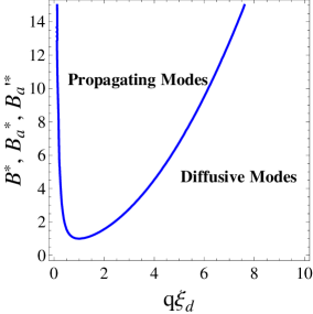
Figure 1: The critical line $B^{*}(\tilde{q})$ given in Eq. (23) for $\epsilon=1$ separating the region of parameters where density fluctuations in a passive incompressible gel relax diffusively, from the region where the system supports propagating density waves. In the chosen dimensionelss units, the same line also describes the boundary $B_{a}^{*}(\tilde{q})$ obtained for the case $k_{u}\rightarrow\infty$ and boundary $B_{a}^{\prime*}(\tilde{q})$ obtained for the case $k_{u}=0$.

No propagating waves exist for $B<\Gamma^{2}\xi_{d}^{2}/\rho_{0}$, corresponding to the minimum of the curve in Fig. 1. We stress that the modes are always diffusive at the longest wavelengths, when $q\rightarrow 0$. These finite wavevector sound-like waves persist down to very small wavevector in the limit of vanishing friction $\Gamma$ with the surrounding fluid. This is seen by setting $\Gamma=0$ first, followed by the small wavevector approximation. The dispersion relations then take the form

$$\omega_{\pm}^{0}=\pm q\sqrt{\frac{B}{\rho_{0}}}-\imath q^{2}\frac{\eta_{L}}{2\rho_{0}}\;.$$ (24)

These are indeed sound waves propagating at the longitudinal sound speed $\sim\sqrt{B/\rho_{0}}$.

III.1.2 Neglecting bound motor fluctuations ($k_{u}\rightarrow\infty$).

We now proceed to incorporate the effect of motor proteins. We first consider the case of stationary bound motors. This can be obtained in two ways, either by letting $k_{u}\rightarrow\infty$, which corresponds to neglecting bound motor fluctuations, or by letting $k_{u}=0$, which corresponds to neglecting the motor on/off dynamics. In both limits motor activity can yield a contractile instability of the system, but no spontaneous oscillations, as pointed out in Ref. [20].

When $k_{u}\rightarrow\infty$, then $\phi=0$ and the concentration of bound motors is constant, $c_{b}=c_{b0}$. We then obtain a single decoupled equation for fluctuations in the longitudinal displacement (or equivalent, in the network density $\delta\rho$) of the form

$$\left\{-\rho_{0}\omega^{2}+(B-\zeta_{1}\Delta\mu)q^{2}-\imath\omega\left[\Gamma+\eta_{L}q^{2}\right]\right\}u_{L}\;.$$ (25)

In this limit the only effect of motor activity is a contractile reduction of the compressional modulus, which is given by

$$B_{a}=B-\zeta_{1}\Delta\mu\;.$$ (26)

The hydrodynamic modes are identical to those described in the previous subsection, with the replacement $B\rightarrow B_{a}$. If $B_{a}<0$ the imaginary part of the mode $\omega_{L}^{0}$ changes sign, signaling a contractile instability of the system driven by motor activity. When $B_{a}>0$, the modes can be real at finite wavevector, corresponding to propagating waves. The condition for the existence of propagating waves is precisely as given in Eq. (23) for the passive gel, with the replacement $B\rightarrow B_{a}$. A plot of $B^{*}_{a}=B_{a}\rho_{0}/(\Gamma^{2}\xi_{d}^{2})$ as a function of $\tilde{q}$ is that identical to that shown in Fig. 1 for the passive case. We stress that the existence of these propagating density waves is not a consequence of activity. There is in fact a maximum value of activity, given by $\zeta_{1}\Delta\mu_{c}=B-\Gamma\xi_{d}^{2}/\tau_{\Gamma}$, and corresponding to the minimum of the curve plotted in Fig. 1 above which there are no propagating modes. In addition, since $\ell_{\Gamma}\sim\sqrt{B_{a}}$ decreases with increasing activity $\Delta\mu$, the range of wavevectors where propagating waves exist for a fixed $B_{a}^{*}$ decreases with increasing activity and is given by $\Delta\tilde{q}=2[B_{a}^{*}(B_{a}^{*}-1)]^{1/4}$.

III.1.3 Neglecting bound motor dynamics ($k_{u}=0$).

In this case bound motors remain bound at all times and bound motor fluctuations are slaved to network density fluctuations, with $\phi=\delta\rho/\rho_{0}$. The relaxation of longitudinal fluctuations is described by

$$\left\{-\rho_{0}\omega^{2}+\left[B-(\zeta_{1}+\zeta_{2})\Delta\mu\right]q^{2}-\imath\omega\left[\Gamma+\eta_{L}q^{2}\right]\right\}u_{L}=0\;.$$ (27)

and the only effect of static bound motors is a further downward renormalization of the elastic modulus, which is now given by

$$B_{a}^{\prime}=B-(\zeta_{1}+\zeta_{2})\Delta\mu\;.$$ (28)

The modes are again formally identical to those obtained for the passive gel, but with $B\rightarrow B_{a}^{\prime}$. The gel exhibits a contractile instability for $B_{a}^{\prime}<0$ and finite wavevector progating density waves for $B_{a}^{\prime}>0$. Note that the limit where all motors are bound can be obtained for instance after full hydrolysis of ATP to ADP. Myosin has a high affinity to actin, hence in a pure ADP environment it will act as a “permanent” bound crosslinker [34]. In this case, however, there will also be no reduction of the elastic modulus due to activity, hence no contractile instability. In fact muscles become rigid as ATP runs out, which is one of the causes of rigor mortis.

III.1.4 Including bound motors dynamics (finite $k_{u}$).

We now incorporate the dynamics of the bound motors and consider the hydrodynamic modes of the the two coupled equations (16a) and (16b). These yield a cubic eigenvalue equation, given by

$$\!\!\!\!\!\!\imath\rho_{0}\omega^{3}-\omega^{2}(\Gamma+k_{u}\rho_{0}+\eta_{L}q^{2})-\imath\omega\Big{\{}k_{u}(\Gamma+\eta_{L}q^{2})$$ (29)

$$+\left[B-\left(\zeta_{1}+\zeta_{2}\right)\Delta\mu\right]q^{2}\Big{\}}+k_{u}B_{a}q^{2}=0\;.$$

The behavior is now controlled by the competition of two time scale, the network relaxation time $\tau_{\Gamma}=\rho_{0}/\Gamma$ and the time scale $\tau_{on}=k_{u}^{-1}$ characterizing the motors on/off dynamics. Solving perturbatively for small wave numbers q, the three modes are given by

$$\omega_{L}=-\imath\frac{B_{a}}{\Gamma}q^{2}+O(q^{4})\;,$$ (30)

$$\omega_{b}=-\imath k_{u}+\imath q^{2}\frac{\zeta_{2}\Delta\mu}{\Gamma-k_{u}\rho_{0}}+O(q^{4})\;,$$ (31)

$$\omega_{L,\Gamma}=-\imath\frac{\Gamma}{\rho_{0}}+\imath q^{2}\left(\frac{B_{a}}{\Gamma}-\frac{\zeta_{2}\Delta\mu}{\Gamma-k_{u}\rho_{0}}-\frac{\eta_{L}}{\rho_{0}}\right)+O(q^{3})$$ (32)

The mode $\omega_{L}$ describing the relative mass diffusion of network and solvent in the gel is unchanged at small wavevector. Again, it changes sign when $\Delta\mu>B/\zeta_{1}$, corresponding to a contractile instability of the gel that occurs when the active stresses exceed the elastic restoring forces from the passive elements of the polymer network. The other two modes are non-hydrodynamic and always stable at long wavelengths. The mode with relaxation rate $\omega_{b}$ describes the decay of fluctuations in the density of bound motors. The mode with relaxation rate $\omega_{L,\Gamma}$ describes the damping of the network due to its motion with respect to the permeating fluid. Even when the on/off dynamics of the bound motors is taken into account, no spontaneous oscillations are generated by motor activity in the long wavelength limit. Oscillatory solutions do, however, occur at finite wavevector, as described below. We note that, although the modes always remain stable, the coupling to motor activity can yield a change in sign of the ${\cal O}(q^{2})$ damping in $\omega_{b}$ and $\omega_{L,\Gamma}$. This effective ”negative viscosity” due to motors occurs when the time scale of the motor on/off dynamics is fast compared to the frictional relaxation of the network, i.e., for $\tau_{\Gamma}>\tau_{on}$. This ”negative friction” effect of motors will become important below and was also discussed in Prost et al [35].

As in the passive case, the dispersion relations of the hydrodynamic modes of our model viscoelastic gel depend on the order in which the limits $\Gamma\rightarrow 0$ and $q\rightarrow 0$ are taken. Above we considered the small $q$ limit for fixed $\Gamma$. If in contrast we take $\Gamma\rightarrow 0$ first, followed by $q\rightarrow 0$ we obtain propagating modes (for $B_{a}>0$). The mode $\omega_{b}$ describing relaxation of bound motor fluctuations is qualitatively unchanged and takes the form

$$\omega_{b}=-\imath k_{u}-\imath q^{2}\frac{\zeta_{2}\Delta\mu}{k_{u}\rho_{0}}+O(q^{4})\;.$$ (33)

The two modes $\omega_{L}$ and $\omega_{L,\Gamma}$ describing the dynamics of network density fluctuations are replaced by two propagating modes (for $B_{a}>0$), with dispersion relation

$$\omega_{L,\pm}=\pm q\sqrt{\frac{B_{a}}{\rho_{0}}}+\imath\frac{q^{2}}{2\rho_{0}}\left(\eta_{L}-\frac{\zeta_{2}\Delta\mu}{k_{u}}\right)\;.$$ (34)

In contrast to the case of a passive gel or a gel with static bound motors, these oscillatory density waves can now become unstable when the (negative) viscosity induced by the motors overcome the internal viscous dissipation of the network, i.e., for $\zeta_{2}\Delta\mu\tau_{on}\geq\eta_{L}$. Above the critical value of activity defined by the vanishing of the damping in Eq. (34), the propagating waves become unstable and the uniform state is presumably replaced by a state that supports spontaneous oscillations.

III.2 Transverse Modes

The transverse equations  (17) and (18) do not couple to motor dynamics. They yield a cubic eigenvalue equation. There are therefore three transverse modes in the system. Of these two are propagating shear waves, with dispersion relation for small $q$ given by

$$\omega({{\bf q}})=\pm q\sqrt{\frac{\mu}{\rho_{g}}}-\frac{\imath q^{2}}{2\rho_{g}}\left(\eta+\eta_{s}+\frac{\mu\rho_{f}^{2}}{\Gamma\rho_{g}}\right)+\ O(q^{3})\;,$$ (35)

with $\rho_{g}=\rho_{0}+\rho_{f}$ the mass density of the gel. The third transverse mode is a non-hydrodynamic mode with a finite decay rate at ${\bf q}=0$. It describes the relative motion of the polymer network and the permeating fluid. The dispersion relation is given by

$$\omega({\bf q})=-\frac{\imath\Gamma\rho_{g}}{\rho_{0}\rho_{f}}-\frac{\imath q^{2}}{\rho_{g}}\left(\frac{\eta\rho_{0}^{2}+\eta_{s}\rho_{f}^{2}}{\rho_{0}\rho_{f}}-\frac{\mu\rho_{f}^{2}}{\Gamma\rho_{g}}\right)+\ O(q^{4})\;.$$ (36)

Transverse fluctuations always decay and to linear order do not destabilize the stationary homogeneous state. Finally, if $B$ and $\mu$ are comparable, the speed of propagation of the transverse waves given in Eq. (35) is generally much smaller than that of the longitudinal waves given in Eq.  (24), since $\rho_{f}>>\rho_{0}$.

IV Overdamped Dynamics of the Polymer Network : Connection to Muscle Sarcomeres

In the overdamped limit of large friction $\Gamma$, the inertial term in Eq. (13a) is negligible and the relaxational dynamics of the fiber density is controlled by the viscous coupling to the permeating fluid. This is the limit that is relevant to most biological systems, such as muscle sarcomeres. We show here that in this limit the on/off dynamics of bound motor yields an effective inertia that results in spontaneous oscillations even in this overdamped limit.

The approximation of neglecting the inertial terms can be quantified as follows. The inertial term in Eq. (13a) can be neglected relative to the frictional damping from the fluid provided $\rho_{0}\omega^{2}<<\Gamma\omega$ or $\omega<<\Gamma/\rho_{0}\sim\eta/(\xi^{2}\rho_{0})$, which is simply the condition of low Reynolds number for an object of typical size $\xi$ moving in a medium of kinematic viscosity $\eta/\rho_{0}$ at a typical speed $\sim\xi\omega$. A sarcomere of typical rest length $\xi\sim 2.5\ \mu m$ [1], moves in an ambient viscous medium of viscosity $\eta\sim 10\ pN\ s\ \mu m^{-1}$. The mass density $\rho_{0}$ of a sarcomere is approximately $10^{3}kg~{}m^{-3}$ [36]. Inertial effects can be neglected if the velocity of a sarcomere unit, typically of order $10\ \mu m\ s^{-1}$, is small compared to $\eta/\xi\rho_{0}$. From the known values of sarcomere parameters, as quoted above, $\eta/\xi\rho_{0}\sim 10^{-2}ms^{-1}$, which is three orders of magnitude higher than the typical velocity of a sarcomere. Hence the ignoring of the inertial forces is justified.

A sarcomere chain can be described as a one dimensional elastic system in terms of a displacement field $u(z,t)$, with $z$ the coordinate along the sarcomere’s length. In the overdamped limit the equation for the displacement field and the deviation of the fraction of bound motor from the steady state value are given by

$$\left(\Gamma-\eta_{L}\partial_{z}^{2}\right)\partial_{t}u=B_{a}\partial_{z}^{2}u+\zeta_{2}\Delta\mu\partial_{z}\phi\;,$$ (37)

$$\partial_{t}\phi=-\partial_{z}\left[\left(1+\phi\right)\partial_{t}{u}\right]-k_{u}\phi\;.$$ (38)

We note that in the overdamped limit discussed in this section our model is formally similar to the model introduced by Murray and Oster [37] to describe the role of the mechanochemistry of the cytogel in epithelium movements (albeit with calcium dynamics taking the place of motor dynamics), but with one important difference: here we consider a gel frictionally coupled to a permeating fluid, while Refs. [37, 38] consider a gel elastically coupled to a substrate. As shown below, both models yield oscillations and traveling waves.

When linearized by approximating the convective term on the right hand side of Eq. (38) as $\sim-\partial_{z}\partial_{t}{u}$, these equations are identical to those derived by Günther-Kruse [20] from a microscopic model of muscle sarcomeres. Here we show that the same equations can be obtained by a purely phenomenological approach that includes both the dissipation due to the coupling to the permeating fluid and the on/off motor dynamics. We also note that the bound motor fraction can be eliminated from the linearized equations by transforming them into a single differential equation for the displacement. Solving the linearized form of Eq. (38) for $\phi$ with $\phi(z,t=0)=0$, substituting in Eq (37) and differentiating with respect to time, we obtain a single differential equation for the displacement $u(z,t)$, albeit second order in time, given by

$$\tau_{on}\left(\Gamma-\eta_{L}\partial_{z}^{2}\right)\partial_{t}^{2}u+\left[\Gamma-\eta_{L}\partial_{z}^{2}-\eta_{a}\partial_{z}^{2}\right]\partial_{t}u=B_{a}\partial_{z}^{2}u$$ (39)

where

$$\eta_{a}=\tau_{on}\left[B-\left(\zeta_{1}+\zeta_{2}\right)\Delta\mu\right]\;.$$ (40)

It is clear from Eq. (39) that the effect of motor on/off dynamics is to provide an ”inertial” contribution to the dynamics of the network. On length scales large compared to $\xi_{d}$ we can neglect the internal dissipation intrinsic to the network proportional to the viscosity $\eta_{L}$ compared to the friction $\Gamma$ with the permeating fluid. Eq. (39) then simplifies to

$$\tau_{on}\Gamma\partial_{t}^{2}u+\left[\Gamma-\eta_{a}\partial_{z}^{2}\right]\partial_{t}u=B_{a}\partial_{z}^{2}u$$ (41)

In this limit Eq. (41) describing deformations of the active network is formally identically to Eq. (19) for the passive gel, with $\tau_{on}\Gamma$ playing the role of a mass density, and a viscosity $\eta_{a}$ and an elastic modulus $B_{a}$, both renormalized by activity. The effective viscosity and the elastic modulus can change sign at high activities, yielding instabilities.

First we consider the hydrodynamic modes of the systems described by the linearized form of Eqs. (37) and (38) or by Eq. (39). These are given by the solutions of the eigenvalue equation, given by

$$\omega^{2}(\Gamma+\eta_{L}q^{2})+\imath\omega k_{u}\left[\Gamma+\left(\eta_{L}+\eta_{a}\right)q^{2}\right]-k_{u}B_{a}q^{2}=0\;.$$ (42)

The general solutions of the eigenvalue equation are

$$\!\!\!\!\omega=\frac{k_{u}}{2(\Gamma+\eta_{L}q^{2})}\Big{\{}-\imath\left[\Gamma+\left(\eta_{L}+\eta_{a}\right)q^{2}\right]$$ (43)

$$\pm\sqrt{-\left[\Gamma+\left(\eta_{L}+\eta_{a}\right)q^{2}\right]^{2}+\frac{4B_{a}q^{2}}{k_{u}}(\Gamma+\eta_{L}q^{2})}\Big{\}}$$

For small wavevector ($q\rightarrow 0$) we obtain two modes,

$$\omega_{b}=-\imath k_{u}+\imath\frac{\zeta_{2}\Delta\mu}{\Gamma}q^{2}$$ (44)

$$\omega_{L}=-\imath\frac{B_{a}}{\Gamma}q^{2}$$ (45)

describing motor and network density relaxation, respectively. Again, the system exhibit a contractile instability when $B_{a}<0$, but there are no oscillatory waves in the long wavelength limit.

Propagating wave solutions exist if the argument of the square root on the right hand side of Eq. (43) is positive. The active viscosity can be written as $\eta_{a}=(B_{a}-\zeta_{2}\Delta\mu)/k_{u}$, hence it depends on the renormalized elastic modulus $B_{a}$. If we choose to treat $\tilde{B}_{a}=B_{a}/(\Gamma\xi_{d}^{2}k_{u})$ and $\tilde{\zeta}_{2}=\zeta_{2}\Delta\mu/(\Gamma\xi_{d}^{2}k_{u})$ as independent parameters the condition for existence of propagating waves can be written as $\tilde{B}_{a}^{-}(\tilde{q})\leq\tilde{B}_{a}\leq\tilde{B}_{a}^{+}(\tilde{q})$, with

$$\tilde{B}_{a}^{\pm}(\tilde{q})=\frac{1}{\tilde{q}^{2}}\left[1+\tilde{q}^{2}+\tilde{\zeta}_{2}\tilde{q}^{2}\pm 2\sqrt{\tilde{q}^{2}(1+\tilde{q}^{2}+\tilde{\zeta}_{2}\tilde{q}^{2})}\right]\;,$$ (46)

where we assumed $\eta_{L}\sim\Gamma\xi_{d}^{2}$. Propagating waves then exist in a band in the $(\tilde{B}_{a},\tilde{q})$ plane, as shown in Fig. 2. The width of the band is $\Delta\tilde{B}_{a}=4\sqrt{1+\tilde{\zeta}_{2}+1/\tilde{q}^{2}}$. It vanishes at small wavevectors and goes to the constant value $4(1+\tilde{\zeta}_{2})^{1/2}$ at large wavevectors. In contrast to the propagating density waves obtained in a damped passive gel, the oscillatory behavior results here from motor activity and the range of parameter where it exists grows with the time $\tau_{on}$ that characterizes motor dynamics. Since $\tau_{on}\sim 1/\Delta\mu$ to leading order $\tilde{\zeta}_{2}$ is independent of activity for small activity. In addition, the propagating waves are unstable when the imaginary part of the eigenvalues given by Eq. (43) is positive. This corresponds to

$$\tilde{B}_{a}\leq\tilde{\zeta}_{2}-\frac{1+\tilde{q}^{2}}{\tilde{q}^{2}}$$ (47)

and defines a region where the overdamped active gel exhibits an oscillatory instability. We expect that when nonlinear terms are included in the equations, the gel will exhibit spontaneous oscillations in this region of parameters.

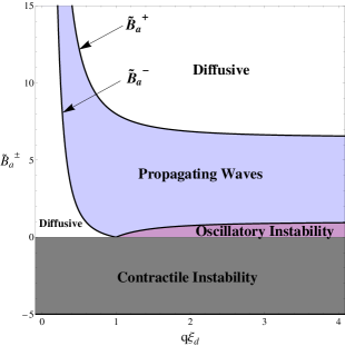
Figure 2: A phase diagram for the overdamped active gel. The vertical axis is $\tilde{B}_{a}=B_{a}/(\Gamma\xi_{d}^{2}k_{u})$ and the horizontal axis is $q\xi_{d}$. The boundaries separating the regions of diffusive relaxation of network density fluctuations from the region where traveling waves exist are given by Eq. (46), plotted here for $\tilde{\zeta}_{2}=2$. Below the horizontal line $\tilde{B}_{a}=0$, the system exhibits a contractile instability.

The transition from diffusive to oscillatory behavior is controlled by the interplay between $\tau_{on}$ and the characteristic time $\tau_{d}\sim\xi_{d}^{2}\Gamma/B$ for the diffusive relaxation of a network fluctuation of size $\xi_{d}$. If $\tau_{on}\gg\tau_{d}$ the on/off motor dynamics provides an ”inertial drag” to the network that opposes the elastic restoring forces, yielding propagating waves. Alternatively, the result can be understood in terms of two length scales in the problem, $\xi_{d}$ and $l_{b}\sim\sqrt{B/(k_{u}\Gamma)}$. If $\xi_{d}>l_{b}$ then density relaxation is always diffusive in the range of wavevectors ($q\xi_{d}\ll 1$) described by the present theory. If in contrast $l_{b}>\xi_{d}$ the network supports propagating density waves in the wavevector range $l_{b}^{-1}\leq q\leq\xi_{d}^{-1}$.

V Linear Response

V.1 Dynamic Compressional Moduli

In this section we characterize the macroscopic homogeneous viscoelastic response of the active gel in frequency space in terms of the dynamical compressional modulus. To describe a traditional compressional experiment, we consider a slab the three-fluid active gel model with only longitudinal degrees of freedom, held between two plates at $z=0$ and $z=L$ and unbounded in the other two directions. We imagine applying a harmonic compressive strain at one end, where $u(z=L)=u_{0}e^{-\imath\omega t}$, while holding the other end fixed, i.e., $u(z=0)=0$. In general, both the cases of an oscillating boundary that is permeable or impermeable to the permeating fluid are experimentally relevant. To implement a calculation that allow to treat both cases one needs to include a finite compressibility so that the longitudinal elasticity equations couple to the fluid velocity $v$. Here we limit ourselves to a permeable boundary and impose no boundary conditions on $v$. With these boundary conditions we calculate the stress $\sigma(z=L)$ required at the oscillating boundary and define the complex compressional modulus $B_{expt}(\omega)$ measured in experiments as the ratio of the stress to the applied compressional strain, $u_{0}/L$. We will see below that at low frequency we recover the complex bulk compressional modulus, $B(\omega)=B-\imath\omega\eta_{L}$, obtained assuming an affine compression over the entire sample.

First we analyze for comparison the case of the passive gel with inertia and damping. The elastic response is governed by the equation

$$\rho_{0}\partial_{t}^{2}u+\Gamma\partial_{t}u=B\partial_{z}^{2}u+\eta_{L}\partial_{t}\partial_{z}^{2}u\;.$$ (48)

We assume a solution of the form $u(z,t)=f(z)e^{-\imath\omega t}$, where $f(z)=f_{i}e^{\lambda_{i}z}$, yielding a characteristic equation for the eigenvalues $\lambda$,

$$\lambda^{2}=-\frac{\omega^{2}\rho_{0}+\imath\omega\Gamma}{B(\omega)}$$ (49)

Boundary conditions, $f(0)=0$ and $f(L)=u_{0}$ lead to the solution,

$$f(z)=u_{0}\frac{\sinh{(\lambda z)}}{\sinh{(\lambda L)}}$$ (50)

The complex dynamic compressional modulus is then given by $B_{exp}(\omega)=\frac{L}{u_{0}}B(\omega)\left(\frac{df}{dz}\right)_{z=L}$ which gives

$$B_{expt}(\omega)=B(\omega)\lambda L\coth{(\lambda L)}$$ (51)

The eigenvalue can be written as

$$\lambda^{2}L^{2}=-\left[\frac{\omega L}{v_{s}(\omega)}\right]^{2}+i\left[\frac{L}{\delta(\omega)}\right]^{2}$$ (52)

where we have defined the frequency dependent sound speed, $v_{s}(\omega)=\sqrt{B(\omega)/\rho_{0}}$, and the penetration depth $\delta(\omega)=\sqrt{B(\omega)/\omega\Gamma}$ which controls the penetration of rarefaction/compression waves of frequency $\omega$ [39]. At low frequency, where $|\lambda L|\ll 1$, we recover $B_{expt}(\omega)\rightarrow B(\omega)$, provided $\omega L/v_{s}(\omega)\ll 1$ and $L\ll\delta(\omega)$. The first condition means that the frequency of applied oscillations is small compared to the frequency of sound wave propagation across the entire sample. When this is not satisfied there is an appreciable time lag between the imposed deformation at one end of the sample and the deformations realized at other material points across the sample, resulting in nonuniform strain and preventing the experimental determination of a macroscopic compressional modulus. The second condition demands that the boundary compressional waves fully penetrated the sample, which is again necessary to achieve a uniform compressional strain. For a similar discussion of shear rheological experiments see Appendix C of Ref. [31]. Finally, the compressional modulus to second order in frequency as measured in a macroscopic experiment is given by

$$B_{expt}(\omega)=B-\omega^{2}\rho_{0}L^{2}/3-\imath\omega(\eta_{L}+\Gamma L^{2}/3)+O(\omega^{3})$$ (53)

We now turn to the compressional response of an active gel. In this case we ignore the inertial contributions relative to the damping from the permeating fluid and look for solutions of the linearized version of Eqs. (37) and (38) of the form $u(z=L)=u_{0}e^{-\imath\omega t}$ and $\phi(z,t)=g(z)e^{-\imath\omega t}$, with $f(z)=f_{i}e^{\lambda_{i}z}$ and $g(z)=g_{i}e^{\lambda_{i}z}$. The eigenvalues are given by

$$\lambda^{2}L^{2}=-i\left[\frac{L}{\delta_{a}(\omega)}\right]^{2}\left[1+\frac{\imath\omega\zeta_{2}\Delta\mu/B_{a}(\omega)}{-\imath\omega+k_{u}}\right]^{-1}\;,$$ (54)

where $\delta_{a}(\omega)=\sqrt{B_{a}(\omega)/\omega\Gamma}$ and $B_{a}(\omega)=B_{a}-i\omega\eta_{L}$. Using, $-\imath\omega f^{\prime}(z)=(-\imath\omega+k_{u})g(z)$ and the boundary conditions on $f(z)$ and proceeding as in the passive case, we obtain

$$B_{expt}^{a}(\omega)=\left[B_{a}(\omega)+\zeta_{2}\Delta\mu\frac{i\omega\tau_{on}}{1-i\omega\tau_{on}}\right]\lambda L\coth{(\lambda L)}\;.$$ (55)

The real and imaginary parts of $B_{expt}^{a}(\omega)=B^{\prime}_{expt}(\omega)-iB^{\prime\prime}_{expt}(\omega)$ representing the storage and loss moduli, respectively, are shown in Fig.(3) for generic values of parameters. The storage or elastic modulus has a frequency independent plateau at frequencies lower than the motor’s unbinding rate, indicating that the system behaves like an elastic gel in this region. The linear frequency dependence of the loss modulus is the hallmark of a dissipative gel. At low frequency $B^{\prime}_{expt}>B^{\prime\prime}_{expt}$ and the system behaves elastically, while at high frequency $B^{\prime\prime}_{expt}>B^{\prime}_{expt}$ and the response is dominated by viscous losses. This response is reminiscent of the Kelvin-Voigt model of viscoelasticity.

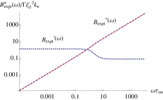
Figure 3: Storage ($B_{expt}^{\prime}(\omega)$) and loss ($B_{expt}^{\prime\prime}(\omega)$) moduli, for $\tilde{B}_{a}=1.15$, $\tilde{\zeta}_{2}=1.1$ and $\xi_{d}/L=0.5$.

Finally, at low frequency the compressional modulus is given by

$$B_{expt}^{a}(\omega) = B_{a}-\omega^{2}\tau_{on}^{2}\zeta_{2}\Delta\mu-i\omega\left(\eta_{L}+\frac{\Gamma L^{2}}{3}-\tau_{on}\zeta_{2}\Delta\mu\right)$$ (56)

$$+O(\omega^{3})\;,$$

whereas, at high frequencies since $\lambda\sim\sqrt{\Gamma/\eta_{L}}=1/\xi_{d}$, we obtain

$$B_{expt}^{a}(\omega)\sim\left(B_{a}-\zeta_{2}\Delta\mu-\imath\omega\eta_{L}\right)(L/\xi_{d})\coth{(L/\xi_{d})}\;.$$ (57)

V.2 Creep

Here we study the macroscopic behavior of our active elastic medium by considering the creep response, i.e., the time evolution of the average strain $\varepsilon(t)=1/L\int_{0}^{L}dz\ \partial_{z}u$ in response to a homogeneous external stress, $\sigma(t)$. In particular we are interested in characterizing the load and recovery creep of the material following the sudden application and removal, respectively, of a constant stress. Both responses are measured experimentally in cells [40, 41, 42].

Consider a muscle fiber of length $L$ with free boundary conditions at the ends $z=0$ and $z=L$, i.e. $\partial_{z}u(z=0,L)=0$, and no fluctuation in motor densities being imposed at the ends. Hence one assumes normal mode expansions for $u$ and $\phi$ to be of the form $u(z,t)=\sum_{m=0}^{\infty}u_{m}(t)\cos{(\hat{m}z)}$, and $\phi(z,t)=\sum_{m=1}^{\infty}\phi_{m}(t)\sin{(\hat{m}z)}$, where $\hat{m}=m\pi/L$.

Neglecting nonlinearities, the evolution of the normal modes $u_{m}(t)$ and $\phi_{m}(t)$ in the material in response to a small external stress $\sigma(t)$ is governed by the equations

$$(\Gamma+\eta_{L}\hat{m}^{2})\dot{u}_{m}(t)+B_{a}\hat{m}^{2}u_{m}(t)-\zeta_{2}\Delta\mu\hat{m}\phi_{m}(t)=f_{m}(t)\;,$$ (58a)

$$\dot{\phi}_{m}(t)=\hat{m}\dot{u}_{m}(t)-k_{u}\phi_{m}(t)\;.$$ (58b)

With, $f_{m}(t)=\frac{2\sigma(t)}{L^{2}}\int_{0}^{L}dz\sin{(\hat{m}z)}$.

Eliminating the fluctuations $\phi_{m}(t)$ in the density of bound motor, we obtain an effective equation for $u_{m}(t)$, given by

$$\begin{split}\tau_{on}(\Gamma+\eta_{L}\hat{m}^{2})\ddot{u}_{m}(t)+\left[\hat{m}^{2}\left(\tau_{on}(B_{a}-\zeta_{2}\Delta\mu)+\eta_{L}\right)+\Gamma\right]\dot{u}_{m}(t)&\\ +B_{a}\hat{m}^{2}u_{m}(t)=\tau_{on}\dot{f}_{m}+f_{m}\;,\end{split}$$ (59)

where $\tau_{on}=k_{u}^{-1}$. The decay rates of the individual modes are

$$2\gamma(m)=k_{u}+\frac{B_{a}-\zeta_{2}\Delta\mu}{\eta_{L}\left(1+\frac{L^{2}}{m^{2}\xi_{d}^{2}\pi^{2}}\right)}\;.$$ (60)

Eq. (60) shows that $\gamma(m)$ is an increasing function of $m$, hence the higher modes decay at a faster rate. For simplicity we then consider only the first mode, $m=1$. Thus we approximate the averaged strain developed in the material as $\varepsilon(t)\simeq-2u_{1}\pi/L$. Also note that neglecting viscous coupling to the fluid $\Gamma$ amounts to considering the limit of the fastest mode $m\rightarrow\infty$.

In the limit $\tau_{on}\rightarrow 0$, when motors are unbound at all times, Eq. (59) reduces to the familiar Kelvin-Voigt viscoelastic equation [43]. In this case the creep following application of a sudden load at $t=0$, $\sigma(t)=\sigma_{0}\Theta(t)$ has the familiar form

$$\varepsilon(t)=\frac{8\sigma_{0}/\pi}{\eta_{L}\pi^{2}+\Gamma L^{2}}(1-e^{-t/(\tau_{B}+\Gamma L^{2}/\pi^{2}B_{a})})\;,$$

where $\tau_{B}=\eta_{L}/B_{a}$ is the Kelvin-Voigt relaxation time.

For finite values of $\tau_{on}$, the creep response is controlled by the interplay of the two times scales $\tau_{B}$ and $\tau_{on}$. We assume $B_{a}>0$, corresponding to weak activity. When $B_{a}<0$ the system exhibits a contractile instability and the strain becomes arbitrarily large at long times for any applied $\sigma(t)$. The evolution of the strain in response to an applied stress is then controlled by the two eigenvalues of Eq. (59) for $m=1$, given by

$$\lambda_{\pm}=-\gamma\pm\sqrt{\gamma^{2}-\frac{\tau_{B}}{J(L)\tau_{on}}}\;,$$ (61)

where time is measured in units of $\tau_{B}$, and

$$2\gamma=\left(1-\frac{\zeta_{2}\Delta\mu}{B_{a}}+\frac{\tau_{B}}{\tau_{on}}+\frac{\Gamma L^{2}}{\pi^{2}B_{a}\tau_{on}}\right)/J(L),$$

$$J(L)=\left[1+\left(\frac{L}{\pi\xi_{d}}\right)^{2}\right].$$

The linear creep response of the active gel can then be classified as follows:

I. $\gamma>0$ , $\gamma^{2}>\frac{\tau_{B}}{J(L)\tau_{on}}$ : stable monotonic behavior

II. $\gamma>0$ , $\gamma^{2}<\frac{\tau_{B}}{J(L)\tau_{on}}$ : stable oscillatory behavior

III. $\gamma=0$ : sustained oscillations

IV. $\gamma<0$ , $\gamma^{2}>\frac{\tau_{B}}{J(L)\tau_{on}}$ : unstable oscillatory growth

V. $\gamma<0$ , $\gamma^{2}<\frac{\tau_{B}}{J(L)\tau_{on}}$ : unstable monotonic growth

The behavior is summarized in the phase diagram of Fig. 4 displaying the various regions in the $(\tau_{on},\zeta_{2})$ plane for fixed $J(L)$. We note that when $\tau_{on}/\tau_{B}$ is increased for fixed $\zeta_{2}\Delta\mu/B_{a}\geq 1$, the material eventually becomes unstable to stretching.

Figure 4: A phase diagram displaying the various types of creep response obtained for $B_{a}>0$. I) Stable Monotonic Decay, II) Stable Oscillatory, III) Line of Sustained Oscillations, IV) Unstable Oscillatory Growth, V) Unstable Monotonic Growth.

Figures  5(a) and 5(b) show the time evolution of the strain in response to a step stress of height $\sigma_{0}$ and duration $T$, $\sigma(t)=\sigma_{0}\left[\Theta(t)-\Theta(t-T)\right]$, with initial condition $\varepsilon(0)=0$. The response in region I of stable monotonic decay is similar to conventional Kelvin-Voigt response. In region II of stable oscillatory decay the interplay of the two time scales $\tau_{on}$ and $\tau_{B}$ yields the possibility of a strain overshoot. For finite $\tau_{on}$ we also need to specify an additional initial condition determined by the initial distribution of bound motors, since $\dot{\varepsilon}(0)=\dot{\phi}(0)-\phi(0)/\tau_{on}$. Fig.  5(b) displays the response in region III of sustained oscillations.

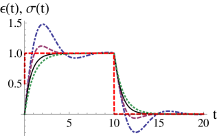
(a)

(b)

Figure 5: (color online) Strain $\varepsilon(t)$ in response to a step-stress $\sigma(t)$ (dashed line, red online) with $T=10$. Strain and stress are measured in units of $\sigma_{0}$ and $\sigma_{0}/B_{a}$, respectively and time is in unites of $\tau_{B}$. The various curves correspond to different values of $\tau_{on}$, spanning the regimes described above. Top frame: $\tau_{on}=0$ (dotted line, green online), corresponding to a passive gel with Kelvin-Voigt response; $\tau_{on}/\tau_{B}=0.2$ (solid line, black online), corresponding to region I of monotonic stable response; $\tau_{on}/\tau_{B}=0.5$ (dashed line, purple online), and $\tau_{on}/\tau_{B}=1$ (dashed-dotted line, blue online), corresponding to region II of oscillatory stable response. All curves are for $\zeta_{2}/B_{a}=1$. Bottom frame: $\tau_{on}/\tau_{B}=0.5$ and $\zeta_{2}/B_{a}=3$, corresponding to region III of sustained oscillations.

VI Discussion and conclusions

We have presented a generic continuum theory of active gels, modeled as a viscoelastic solid with bound motor proteins that induce active stresses in the medium. In the limit where the inertia of the network is neglected and the equations are specialized to one dimension, the model is equivalent to that proposed by Günther and Kruse [20] by coarse-graining of a specific mechanical model of coupled muscle sarcomeres. For large values of the motor activity as measured by the rate of ATP consumption, $\Delta\mu$, the contractile action of bound motors yields a diffusive (contractile) instability of the gel. This result has been obtained earlier in models of muscle sarcomeres [20] and actin bundles [44]. Here we show that it is a generic property of active elastic media. For smaller values of motor activity the interplay of solid elasticity and the binding/unbinding dynamics of the motor proteins yields propagating waves and eventually oscillatory instabilities in the linear theory. Both stable and unstable oscillatory modes are obtained even in the case of an overdamped gel, as relevant to muscle fibers. We show that the finite time scale of motor on/off dynamics yields an effective ”inertial” contribution to the dynamics of the elastic medium controlled by the time $\tau_{on}$ that motors spend bound to filaments (see Eq. (39)). One of the new results of the paper is the phase diagram displayed in Fig. 4 for the macroscopic response of the system to external stresses. In the linear model sustained oscillations are only obtained for special parameter values corresponding to a line in the $(\tau_{on},\zeta_{2})$ phase diagram. It is expected that nonlinearities neglected in the present work will have a stabilizing effect and replace the unstable oscillatory response with stable self-sustained oscillations. The model considered is relevant for the description of motor-induced spontaneous oscillations in muscle sarcomeres and other active elastic media, and may provide a useful framework for the understanding of lamellipodium crawling.

We plan to extend this work in various ways. First, an analysis of the effect on nonlinearities is needed. Two classes of nonlinear terms are important in our model of an active gel. The first is provided by nonlinear convective terms in the equation describing the dynamics of bound motors, as shown in Eq. (38), and also including dependence of the unbinding rate $k_{u}$ on the elastic strain $\partial_{z}u$ developed in the gel. These are the simplest continuum manifestation of the highly nonlinear load dependence of the microscopic motor unbinding rate, which in turn plays an important role in controlling the motor-induced negative friction induced by the cooperative action of motor proteins on biological systems elastically coupled to their environment [35, 30, 45]. A second class of nonlinearities arise from higher order terms in the expansion of the active parameter $\zeta$ given in Eq. (7). A preliminary estimate of the effect of these terms suggest that they stabilize the oscillatory growing modes and yield stable sustained oscillations.

In the liquid state of an active system the polarity of actin filaments plays an important role. The coupling of polarity and flow has been shown to yield spontaneous flow [6], banded states of inhomogeneous concentration, and oscillatory states [7]. It is similarly expected that the coupling of polarity and elasticity will yield new phenomena in active solids, including spontaneous deformations and oscillations. To incorporate the effect of polarity we have begun to consider the properties of an active polar elastomer, where the orientational order can be induced either by elongated passive crosslinkers [46] or by the myosin minifilaments themselves. In addition, the latter exert active force dipoles on the medium that induce active stresses coupled to the orientational order. A detailed discussion and analysis of such active elastomers is left for a future publication.

We acknowledge support from the NSF on grants DMR-075105 and DMR-0806511. We thank Aparna Baskaran, Alex Levine, Tannie Liverpool and Kristian Müller-Nedebock for illuminating discussions. SB also thanks the University of Stellenbosch for hospitality during the completion of part of this work.

References

- [1] B. Alberts and A. Johnson and J. Lewis and M. Raff and K. Roberts and P. Walter, Molecular biology of the cell, 5th ed., Garland, New York, 2007.
- [2] J. Howard, Mechanics of motor proteind and the cytoskeleton, Sinauer, New York, 2000.
- [3] K. Kruse, J. F. Joanny, F. Jülicher, J. Prost, and K. Sekimoto, Phys. Rev. Lett., 2004, 92, 078101.
- [4] K. Kruse. J. F. Joanny, F. Jülicher, J. Prost and K. Sekimoto, Eur. Phys J. E, 2005, 16, 5.
- [5] F. Jülicher, K. Kruse, J. Prost and J.-F. Joanny, Phys. Rep., 2007, 449, 3-28.
- [6] R. Voituriez, J. F. Joanny and J. Prost, Europhys. Lett., 2005, 70, 118102.
- [7] L. Giomi, M. C. Marchetti and T. B. Liverpool, Phys. Rev. Lett., 2008, 101, 198101.
- [8] F. J. Nédédlec, T. Surrey, A. C. Maggs and S. Leibler, Nature, 1997, 389, 305-308.
- [9] T. Surrey, F. Nédélec, S. Leibler and E. Karsenti, Science, 2001, 292, 1167-1171.
- [10] I. S. Aranson and L. S. Tsimring, Phys. Rev. E, 2005, 71, 050901.
- [11] I. S. Aranson and L. S. Tsimring, Phys. Rev. E, 2006, 74, 031915.
- [12] T.B. Liverpool and M.C. Marchetti, Phys. Rev. Lett., 2003, 90, 138102.
- [13] A. Ahmadi, T.B. Liverpool and M.C. Marchetti, Phys. Rev. E, 2005, 72, 060901.
- [14] Y. Hatwalne, S. Ramaswamy, M. Rao and R. A. Simha, Phys. Rev. Lett., 2004, 92, 118101.
- [15] T. B. Liverpool and M. C. Marchetti, Phys. Rev. Lett., 2006, 97, 268101.
- [16] L. Giomi, T. B. Liverpool and M. C. Marchetti, Phys. Rev. E, 2010, 81, 051908.
- [17] M. E. Cates, S. M. Fielding, D. Marenduzzo, E. Orlandini, and J. M. Yeomans, Phys. Rev. Lett., 2008, 101, 068102.
- [18] S. Pellegrin and H. Mellor, J. Cell Sci., 2007, 120, 3491-3499.
- [19] T. Anazawa, K. Yasuda and S. Ishiwata, Biophys. J., 1992, 61, 1099.
- [20] S. Günther and K. Kruse, New J. Phys., 2007, 9, 417.
- [21] F. Jülicher and J. Prost, Phys. Rev. Lett., 1997, 78, 5410.
- [22] M. Rubinstein and R. H. Colby, Polymer Physics, Oxford University Press Inc., New York, 2003, p. 199.
- [23] D. Mizuno, C. Tardin, C. F. Schmidt and F. C. MacKintosh, Science, 2007, 315 , 370.
- [24] F. C. MacKintosh and A. J. Levine, Phys. Rev. Lett., 2008, 100, 018104.
- [25] A. J. Levine and F. C. MacKintosh, J. Phys. Chem. B, 2009, 113, 3820.
- [26] T. B. Liverpool, M. C. Marchetti, J.-F. Joanny and J. Prost, Eur. Phys. Lett., 2009, 85, 18007.
- [27] C. J. Brokaw, Proc. Nat. Acad. Sci. USA, 1975, 72, 3102.
- [28] S. Camalet, F. Jülicher and J. Prost, Phys. Rev. Lett., 1999, 82, 1590.
- [29] S. Camalet and F. Jülicher, New J. Phys., 2000, 2, 1.
- [30] S. Grill, K. Kruse and F. Jülicher, Phys. Rev. Lett., 2005, 94, 108104.
- [31] A.J. Levine and T.C. Lubensky, Phys. Rev E, 2001, 63 041510.
- [32] A. J. Levine and T. C. Lubensky, Phys. Rev. Lett., 2000, 85, 1774.
- [33] D.A. Head and D. Mizuno, Phys. Rev. E., 2010, 81, 041910.
- [34] D. Humphrey, C. Duggan, D. Saha, D. Smith and J. Käs, Nature, 416, 412.
- [35] F. Jülicher and J. Prost, Phys. Rev. Lett., 1995, 75, 2618.
- [36] J. Denoth, E. Stüssi, G. Csucs, and G. Danuser, J. Theor. Biol., 2002, 216, 101.
- [37] J.D. Murray and G.F. Oster, Math. Med. Biol., 1984, 1, 51.
- [38] G. M. Odell, G. Oster, P. Alberch and B. Burnside, Dev. Biol., 1981, 85, 446.
- [39] A.J. Levine and F.C. MacKintosh, J. Phys. Chem. B, 2009, 113, 3820.
- [40] T. W. Bartel and S. L. Yaniv, J. Res. Natl. Inst. Stand. Technol., 1997, 102, 349.
- [41] O. Thoumine and A. Ott, J. Cell Sci., 1997, 110, 2109.
- [42] D. Mitrossilis, J. Fouchard, A. Guiroy, N. Desprat, N. Rodriguez, B. Fabry, and A. Asnacios, Proc. Nat. Ac. Sci., 2009, 106, 18243.
- [43] A. S. Wineman and K. R. Rajagopal, Mechanical response of polymers : An introduction, Cambridge University Press, Cambridge, England; New York, 2000.
- [44] R. Peter, V. Schaller, F. Ziebert and W. Zimmermann, New J. Phys., 2008, 10, 035002.
- [45] P.-Y. Plaçais, M. Balland, T. Guérin, J.-F. Joanny and P. Martin, Phys. Rev. Lett., 2009, 103, 158102.
- [46] P. Dalhaimer, D. E. Discher and T. C. Lubensky, Nature Physics, 2007, 3, 354.