Joint Bandwidth and Power Allocation with Admission Control in Wireless Multi-User Networks With and Without Relaying

Abstract

Equal allocation of bandwidth and/or power may not be efficient for wireless multi-user networks with limited bandwidth and power resources. Joint bandwidth and power allocation strategies for wireless multi-user networks with and without relaying are proposed in this paper for (i) the maximization of the sum capacity of all users; (ii) the maximization of the worst user capacity; and (iii) the minimization of the total power consumption of all users. It is shown that the proposed allocation problems are convex and, therefore, can be solved efficiently. Moreover, the admission control based joint bandwidth and power allocation is considered. A suboptimal greedy search algorithm is developed to solve the admission control problem efficiently. The conditions under which the greedy search is optimal are derived and shown to be mild. The performance improvements offered by the proposed joint bandwidth and power allocation are demonstrated by simulations. The advantages of the suboptimal greedy search algorithm for admission control are also shown.

I Introduction

One of the critical issues in wireless multi-user networks is efficient allocation of available radio resources in order to improve the network performance [1], [2]. Therefore, power allocation strategies in wireless multi-user networks have been extensively studied [3]–[5]. In practical wireless networks, however, both the available transmission power of individual nodes and the total available bandwidth of the network are limited and, therefore, joint bandwidth and power allocation must be considered [6]–[8]. Such joint bandwidth and power allocation is important for both systems with and without relaying. In the case of severe channel conditions in direct links, relays can be deployed to forward the data from a source to a destination in order to improve communication efficiency [9]–[11].

There are numerous works conducted on the resource allocation in wireless relay networks (see, for example, [12]–[14]). Power allocation with the decode-and-forward (DF) protocol has been studied in [12] under the assumption that transmitters only know mean channel gains. In [13], a power allocation scheme that aims at maximizing the smallest of two transceiver signal-to-noise ratios (SNRs) has been studied for two-way relay networks. To optimize effective capacity in relay networks, time/bandwidth allocation strategies with constant power have been developed based on time division multiple access/frequency division multiple access (TDMA/FDMA) in [14]. However, [12]–[14] as well as most of the works on the resource allocation in wireless relay networks consider the case of a single user, i.e., a single source-destination pair.

Resource allocation for wireless multi-user relay networks has been investigated only in few works [15]–[19]. Power allocation aiming at optimizing the sum capacity of multiple users for four different relay transmission strategies has been studied in [17], while an AF based strategy in which multiple sources share multiple relays using power control has been developed in [18], [19].

It is worth noting that the works mentioned above (except [14]) have assumed equal and fixed bandwidth allocation for the one-hop links from a source to a destination. In fact, it is inefficient to allocate the bandwidth equally when the total available bandwidth is limited. Moreover, the problem of joint allocation of bandwidth and power has never been considered for wireless multi-user relay networks.

Various performance metrics for resource allocation in multi-user networks have been considered. System throughput maximization and the worst user throughput maximization are studied using convex optimization in [1]. Sum capacity maximization is taken as an objective for power allocation in [17], while max-min SNR, power minimization, and throughput maximization are used as power allocation criteria in [18].

In some applications, certain minimum transmission rates must be guaranteed for the users in order to satisfy their quality-of-service (QoS) requirements. For instance, in real-time voice and video applications, a minimum rate should be guaranteed for each user to satisfy the delay constraints of the services. However, when the rate requirements can not be supported for all users, admission control is adopted to decide which users to be admitted into the network. The admission control in wireless networks typically aims at maximizing the number of admitted users and has been recently considered in several works. A single-stage reformulation approach for a two-stage joint resource allocation and admission control problem is proposed in [20], [21], while another approach is based on user removals [22], [23].

In this paper, the problem of joint bandwidth and power allocation for wireless multi-user networks with and without relaying is considered, which is especially efficient for the networks with both limited bandwidth and limited power. The joint bandwidth and power allocation are proposed to (i) maximize the sum capacity of all users; (ii) maximize the capacity of the worst user; (iii) minimize the total power consumption of all users. The corresponding joint bandwidth and power allocation problems can be formulated as optimization problems that are shown to be convex. Therefore, these problems can be solved efficiently by using convex optimization techniques. The joint bandwidth and power allocation together with admission control is further considered, and a greedy search algorithm is developed in order to reduce the computational complexity of solving the admission control problem. The optimality conditions of the greedy search are derived and analyzed.

The rest of this paper is organized as follows. System models of multi-user networks without relaying and with DF relaying are given in Section II. In Section III, joint bandwidth and power allocation problems for the three aforementioned objectives are formulated and studied for both types of systems with and without relaying. The admission control based joint bandwidth and power allocation problem is formulated in Section IV, where the greedy search algorithm is also developed and investigated for both types of systems with and without relaying. Numerical results are reported in Section V, followed by concluding remarks in Section VI.

II System Model

II-A Without Relaying

Consider a wireless network, which consists of $M$ source nodes $S_{i}$, $i\in\mathcal{M}=\{1,2,\cdots,M\}$, and $K$ destination nodes $D_{i}$, $i\in\mathcal{K}=\{1,2,\cdots,K\}$. The network serves $N$ users $U_{i}$, $i\in\mathcal{N}=\{1,2,\cdots,N\}$, where each user represents a one-hop link from a source to a destination. The set of users which are served by $S_{i}$ is denoted by $\mathcal{N}_{S_{i}}$.

A spectrum of total bandwidth $W$ is available for the transmission from the sources. This spectrum can be divided into distinct and nonoverlapping channels of unequal bandwidths, so that the sources share the available spectrum through frequency division and, therefore, do not interfere with each other.

Let $P^{\rm S}_{i}$ and $W^{\rm S}_{i}$ denote the allocated transmit power and channel bandwidth of the source to serve $U_{i}$. Then the received SNR at the destination of $U_{i}$ is

$$\gamma^{\rm D}_{i}=\frac{P^{\rm S}_{i}h^{\rm SD}_{i}}{W^{\rm S}_{i}N_{0}}$$ (1)

where $h^{\rm SD}_{i}$ denotes the channel gain of the source–destination link of $U_{i}$ and $W^{\rm S}_{i}N_{0}$ stands for the power of additive white Gaussian noise (AWGN) over the bandwidth $W^{\rm S}_{i}$. The channel gain $h^{\rm SD}_{i}$ results from such effects as path loss, shadowing, and fading. Due to the fact that the power spectral density (PSD) of AWGN is constant over all frequencies with the constant value denoted by $N_{0}$, the noise power in the channel is linearly increasing with the channel bandwidth. It can be seen from (1) that a channel with larger bandwidth introduces higher noise power and, thus, reduces the SNR.

Channel capacity gives the upper bound on the achievable rate of a link. Given $\gamma^{\rm D}_{i}$, the source–destination link capacity of $U_{i}$ is

$$C^{\rm SD}_{i}=W^{\rm S}_{i}\log(1+\gamma^{\rm D}_{i})=W^{\rm S}_{i}\log\left(1+\frac{P^{\rm S}_{i}h^{\rm SD}_{i}}{W^{\rm S}_{i}N_{0}}\right).$$ (2)

It can be seen that $W^{\rm S}_{i}$ characterizes channel bandwidth, and $\log(1+\gamma^{\rm R}_{i})$ characterizes spectral efficiency and, thus, $C^{\rm SD}_{i}$ characterizes data rate over the source–destination link in bits per second. Moreover, for fixed $W^{\rm S}_{i}$, $C^{\rm SD}_{i}$ is a concave increasing function of $P^{\rm S}_{i}$. It can be also shown that $C^{\rm SD}_{i}$ is a concave increasing function of $W^{\rm S}_{i}$ for fixed $P^{\rm S}_{i}$, although $\gamma^{\rm D}_{i}$ is a linear decreasing function of $W^{\rm S}_{i}$. Indeed, it can be proved that $C^{\rm SD}_{i}$ is a concave function of $P^{\rm S}_{i}$ and $W^{\rm S}_{i}$ jointly [6], [7], and [25].

II-B With Relaying

Consider $L$ relay nodes $R_{i}$, $i\in\mathcal{L}=\{1,2,\cdots,L\}$ added to the network described in the previous subsection and used to forward the data from the sources to the destinations. Then each user represents a two-hop link from a source to a destination via relaying. To reduce the implementation complexity at the destinations, single relay assignment is adopted so that each user has one designated relay. Then the set of users served by $R_{i}$ is denoted by $\mathcal{N}_{R_{i}}$. The relays work in a half-duplex manner due to the practical limitation that they can not transmit and receive at the same time. A two-phase decode-and-forward (DF) protocol is assumed, i.e., the relays receive and decode the transmitted data from the sources in the first phase, and re-encode and forward the data to the destinations in the second phase. The sources and relays share the total available spectrum in the first and second phases, respectively. It is assumed that the direct links between the sources and the destinations are blocked and, thus, are not available. Note that although the two-hop relay model is considered in the paper, the results are applicable for multi-hop relay models as well.

Let $P^{\rm R}_{i}$ and $W^{\rm R}_{i}$ denote the allocated transmit power and channel bandwidth of the relay to serve $U_{i}$. The two-hop source–destination link capacity of $U_{i}$ is given by

$$C^{\rm SD}_{i}=\min\{C^{\rm SR}_{i},C^{\rm RD}_{i}\}=\left\{W^{\rm S}_{i}\log\left(1+\frac{P^{\rm S}_{i}h^{\rm SR}_{i}}{W^{\rm S}_{i}N_{0}}\right),\,W^{\rm R}_{i}\log\left(1+\frac{P^{\rm R}_{i}h^{\rm RD}_{i}}{W^{\rm R}_{i}N_{0}}\right)\right\}$$ (3)

where $C^{\rm SR}_{i}$ and $C^{\rm RD}_{i}$ are the one-hop source–relay and relay–destination link capacities of $U_{i}$, respectively, and $h^{\rm SR}_{i}$ and $h^{\rm RD}_{i}$ denote the corresponding channel gains.

It can be seen from (3) that if equal bandwidth is allocated to $W^{\rm S}_{i}$ and $W^{\rm R}_{i}$, $C^{\rm SR}_{i}$ and $C^{\rm RD}_{i}$ can be unequal due to the power limits on $P^{\rm S}_{i}$ and $P^{\rm R}_{i}$. Then the source–destination link capacity $C^{\rm SD}_{i}$ is constrained by the minimum of $C^{\rm SR}_{i}$ and $C^{\rm RD}_{i}$. Note that since all users share the total bandwidth of the spectrum, equal bandwidth allocation for all one-hop links can be inefficient. Therefore, the joint allocation of bandwidth and power is necessary.

III Joint Bandwidth and Power Allocation

Different objectives can be considered while jointly allocating bandwidth and power in wireless multi-user networks. The widely used objectives for network optimization are (i) the sum capacity maximization; (ii) the worst user capacity maximization; and (iii) the total network power minimization. In this section, the problems of joint bandwidth and power allocation are formulated for the aforementioned objectives for both considered systems with and without relaying. It is shown that all these problems are convex and, therefore, can be efficiently solved using standard convex optimization methods.

III-A Sum Capacity Maximization

In the applications without delay constraints, a high data rate from any user in the network is preferable. Thus, it is desirable to allocate the resources to maximize the overall network performance, e.g., the sum capacity of all users.

III-A1 Without Relaying

In this case, the joint bandwidth and power allocation problem aiming at maximizing the sum capacity of all users can be mathematically formulated as

$$\max_{\{P^{\rm S}_{i},W^{\rm S}_{i}\}}\;\sum_{i\in\mathcal{N}}C^{\rm SD}_{i}$$ (4a)

$${\rm s.t.}\sum_{i\in\mathcal{N}_{S_{j}}}P^{\rm S}_{i}\leq P_{S_{j}},\ j\in\mathcal{M}$$ (4b)

$$\quad\ \ \,\sum_{i\in\mathcal{N}}W^{\rm S}_{i}\leq W.$$ (4c)

The nonnegativity constraints on the optimization variables $\{P^{\rm S}_{i},W^{\rm S}_{i}\}$ are natural and, thus, omitted throughout the paper for brevity. In the problem (4a)–(4c), the constraint (4b) stands that the total power at $S_{j}$ is limited by $P_{S_{j}}$, while the constraint (4c) indicates that the total bandwidth of the channels allocated to the sources is also limited by $W$.

Note that since $C^{\rm SD}_{i}$ is a jointly concave function of $P^{\rm S}_{i}$ and $W^{\rm S}_{i}$, the objective function (4a) is convex. The constraints (4b) and (4c) are linear and, thus, convex. Therefore, the problem (4a)–(4c) itself is convex. Using the convexity, the closed-form solution of the problem (4a)–(4c) is given in the following proposition.

Proposition 1: The optimal solution of the problem (4a)–(4c), denoted by $\{{P^{\rm S}_{i}}^{\ast},{W^{\rm S}_{i}}^{\ast}|i\in\mathcal{N}\}$, is ${P^{\rm S}_{i}}^{\ast}={P^{\rm S}_{i}}^{\star}$, ${W^{\rm S}_{i}}^{\ast}=Wh^{\rm SD}_{i}{P^{\rm S}_{i}}^{\star}/\sum_{j\in\mathcal{I}}h^{\rm SD}_{j}{P^{\rm S}_{j}}^{\star}$, $\forall i\in\mathcal{I}$, and ${P^{\rm S}_{i}}^{\ast}={W^{\rm S}_{i}}^{\ast}=0$, $\forall i\notin\mathcal{I}$, where ${P^{\rm S}_{i}}^{\star}=P_{S_{k}}$ for $i\in\mathcal{N}_{S_{k}}$ and $\mathcal{I}=\{i\,|\,i={\rm arg}\max_{j\in\mathcal{N}_{S_{k}}}h^{\rm SD}_{j},k\in\mathcal{M}\}$.

Proof:  See Appendix A.

Proposition 1 shows that for a set of users served by one source, the sum capacity maximization based allocation strategy allocates all the power of the source only to the user with the highest channel gain and, therefore, results in highly unbalanced resource allocation among the users.

III-A2 With Relaying

The sum capacity maximization based joint bandwidth and power allocation problem for the network with DF relaying is given by

$$\max_{\{P^{\rm S}_{i},W^{\rm S}_{i},P^{\rm R}_{i},W^{\rm R}_{i}\}}\;\sum_{i\in\mathcal{N}}C^{\rm SD}_{i}$$ (5a)

$${\rm s.t.}\sum_{i\in\mathcal{N}_{S_{j}}}P^{\rm S}_{i}\leq P_{S_{j}},\ j\in\mathcal{M}$$ (5b)

$$\quad\ \,\sum_{i\in\mathcal{N}_{R_{j}}}P^{\rm R}_{i}\leq P_{R_{j}},\ j\in\mathcal{L}$$ (5c)

$$\quad\ \ \,\sum_{i\in\mathcal{N}}W^{\rm S}_{i}\leq W$$ (5d)

$$\quad\ \ \,\sum_{i\in\mathcal{N}}W^{\rm R}_{i}\leq W.$$ (5e)

Introducing new variables $\{T_{i}|i\in\mathcal{N}\}$, the problem (5a)–(5e) can be equivalently rewritten as

$$\min_{\{P^{\rm S}_{i},W^{\rm S}_{i},P^{\rm R}_{i},W^{\rm R}_{i},T_{i}\}}\quad-\sum_{i\in\mathcal{N}}T_{i}$$ (6a)

$${\rm s.t.}\ T_{i}-C^{\rm SR}_{i}\leq 0,\ i\in\mathcal{N}$$ (6b)

$$\quad\ \ T_{i}-C^{\rm RD}_{i}\leq 0,\ i\in\mathcal{N}$$ (6c)

$$\quad\ \ \textrm{the \ constraints \ \eqref{sumr2}--\eqref{sumr5}}.$$ (6d)

Note that the constraints (6b) and (6c) are convex since $C^{\rm SR}_{i}$ and $C^{\rm RD}_{i}$ are jointly concave functions of $P^{\rm S}_{i}$, $W^{\rm S}_{i}$ and $P^{\rm R}_{i}$, $W^{\rm R}_{i}$, respectively. The constraints (6d) are linear and, thus, convex. Therefore, the problem (6a)–(6d) itself is convex. It can be seen that the closed-form solution of the problem (6a)–(6d) is intractable due to the coupling of the constraints (6b) and (6c). However, the convexity of the problem (6a)–(6d) allows to use standard numerical convex optimization algorithms for solving the problem efficiently [26].

Intuitively, the sum capacity maximization based allocation for the network with DF relaying can not result in significantly unbalanced resource allocation as that for the network without relaying. It is because the channel gains in both transmission phases for the networks with relaying affect the achievable capacity of each user. The following proposition gives the conditions under which the sum capacity maximization based resource allocation strategy for the network with relaying does not allocate any resources to some users.

Proposition 2: If $h^{\rm SR}_{i}\geq h^{\rm SR}_{j}$ and $h^{\rm RD}_{i}\geq h^{\rm RD}_{j}$ where $\{i,j\}\subseteq\mathcal{N}_{S_{k}}$ and $\{i,j\}\subseteq\mathcal{N}_{R_{l}}$, then ${P^{\rm S}_{j}}^{\ast}={W^{\rm S}_{j}}^{\ast}={P^{\rm R}_{j}}^{\ast}={W^{\rm R}_{j}}^{\ast}=0$.

Proof:  See Appendix A.

In particular, if two users are served by the same source and the same relay, and one user has lower channel gains than the other user in both transmission phases, then no resource is allocated to the former user.

III-B Worst User Capacity Maximization

Fairness among users is also an important issue for resource allocation. If the fairness issue is considered, the achievable rate of the worst user is commonly used as the network performance measure. In this case, the joint bandwidth and power allocation problem for the network without relaying can be mathematically formulated as

$$\max_{\{P^{\rm S}_{i},W^{\rm S}_{i}\}}\quad\min_{i\in\mathcal{N}}C^{\rm SD}_{i}$$ (7a)

$${\rm s.t.}\ \textrm{the \ constraints \ \eqref{sum2}--\eqref{sum3} }.$$ (7b)

Similar, for the networks with relaying, the joint bandwidth and power allocation problem can be formulated as

$$\max_{\{P^{\rm S}_{i},W^{\rm S}_{i},P^{\rm R}_{i},W^{\rm R}_{i}\}}\quad\min_{i\in\mathcal{N}}C^{\rm SD}_{i}$$ (8a)

$${\rm s.t.}\ \textrm{the \ constraints \ \eqref{sumr2}--\eqref{sumr5} }.$$ (8b)

Introducing a variable $T$, the problem (8a)–(8b) can be equivalently written as

$$\min_{\{P^{\rm S}_{i},W^{\rm S}_{i},P^{\rm R}_{i},W^{\rm R}_{i},T\}}\quad-T$$ (9a)

$${\rm s.t.}\ T-C^{\rm SR}_{i}\leq 0,\ i\in\mathcal{N}$$ (9b)

$$\quad\ \ T-C^{\rm RD}_{i}\leq 0,\ i\in\mathcal{N}$$ (9c)

$$\quad\ \ \textrm{the \ constraints \ \eqref{sumr2}--\eqref{sumr5}}.$$ (9d)

Similar to the sum capacity maximization based allocation problems, it can be shown that the problems (7a)–(7b) and (9a)–(9d) are convex. Therefore, the optimal solutions can be efficiently obtained using standard convex optimization methods.

The next proposition indicates that the worst user capacity maximization based allocation leads to absolute fairness among users, just the opposite to the sum capacity maximization based allocation. The proof is intuitive from the fact that the total bandwidth is shared by all users, and is omitted for brevity.

Proposition 3: In the problems (7a)–(7b) and (8a)–(8b), the capacities of all users are equal at optimality.

III-C Total Network Power Minimization

Another widely considered design objective is the minimization of the total power consumption of all users. This minimization is performed under the constraint that the rate requirements of all users are satisfied. The corresponding joint bandwidth and power allocation problem for the network without relaying can be written as

$$\min_{\{P^{\rm S}_{i},W^{\rm S}_{i}\}}\quad\sum_{i\in\mathcal{N}}P^{\rm S}_{i}$$ (10a)

$${\rm s.t.}\ c_{i}-C^{\rm SD}_{i}\leq 0,\;i\in\mathcal{N}$$ (10b)

the  constraints  (4b)–(4c) (10c)

while the same problem for the network with relaying is

$$\min_{\{P^{\rm S}_{i},W^{\rm S}_{i},P^{\rm R}_{i},W^{\rm R}_{i}\}}\quad\sum_{i\in\mathcal{N}}(P^{\rm S}_{i}+P^{\rm R}_{i})$$ (11a)

$${\rm s.t.}\ c_{i}-C^{\rm SR}_{i}\leq 0,\;i\in\mathcal{N}$$ (11b)

$$\quad\ \ c_{i}-C^{\rm RD}_{i}\leq 0,\;i\in\mathcal{N}$$ (11c)

the  constraints  (5b)–(5e) (11d)

where $c_{i}$ is the minimum acceptable capacity for $U_{i}$ and the constraints (10b) and (10c) indicate that the one-hop link capacities of $U_{i}$ should be no less than the given capacity threshold. Similar to the sum capacity maximization and worst user capacity maximization based allocation problems, the problems (10a)–(10c) and (11a)–(11d) are convex and, thus, can be solved efficiently as mentioned before.

IV Admission Control Based Joint Bandwidth and Power Allocation

In the multi-user networks under consideration, admission control is required if a certain minimum capacity must be guaranteed for each user. The admission control aims at maximizing the number of admitted users and is considered next for both systems with and without relaying.

IV-A Without Relaying

The admission control based joint bandwidth and power allocation problem in the network without relaying can be mathematically expressed as

$$\max_{\{P^{\rm S}_{i},W^{\rm S}_{i}\},\mathcal{I}\subseteq\mathcal{N}}\quad|\mathcal{I}|$$ (12a)

$$\textrm{s.t.}\ c_{i}-C^{\rm SD}_{i}\leq 0,\ i\in\mathcal{I}$$ (12b)

the  constraint  (4b)–(4c) (12c)

where $|\mathcal{I}|$ stands for the cardinality of $\mathcal{I}$.

Note that the problem (12a)–(12c) can be solved using exhaustive search among all possible subsets of users. However, the computational complexity of the exhaustive search can be very high since the number of possible subsets of users is exponentially increasing with the number of users, which is not acceptable for practical implementation. Therefore, we develop a suboptimal greedy search algorithm that significantly reduces the complexity of finding the maximum number of admissible users.

IV-A1 Greedy Search Algorithm

Consider the following problem

$$G(\mathcal{I})\ \triangleq\ \min_{\{P^{\rm S}_{i},W^{\rm S}_{i}\}}\quad\sum_{i\in\mathcal{I}}W^{\rm S}_{i}$$ (13a)

$$\textrm{s.t.}\ c_{i}-C^{\rm SD}_{i}\leq 0,\ i\in\mathcal{I}$$ (13b)

$$\quad\ \ \textrm{the \ constraint \eqref{sum2}}.$$ (13c)

The following proposition provides a necessary and sufficient condition for the admissibility of a set of users.

Proposition 4: A set of users $\mathcal{I}$ is admissible if and only if $G(\mathcal{I})\leq W$.

Proof:  See Appendix B.

According to Proposition 4, the optimal value $G(\mathcal{I})$ is the minimum total bandwidth required to support the users in $\mathcal{I}$, given that all power constraints are satisfied. This is instrumental in establishing our greedy search algorithm, which removes users one by one until the remaining users are admissible. The ‘worst’ user, i.e., the user whose removal reduces the total bandwidth requirement to the maximum extent, is removed at each greedy search iteration. In other words, the removal of the ‘worst’ user results in the minimum total bandwidth requirement of the remaining users. Thus, the removal criterion can be stated as

$$n{(t)}\triangleq\textrm{arg}\max_{n\in\mathcal{N}{(t-1)}}\left(G(\mathcal{N}{(t-1)})-G(\mathcal{N}{(t-1)}\setminus\{n\})\right)=\textrm{arg}\min_{n\in\mathcal{N}{(t-1)}}G(\mathcal{N}{(t-1)}\setminus\{n\})$$ (14)

where $n{(t)}$ denotes the user removed at the $t$-th greedy search iteration, $\mathcal{N}{(t)}\triangleq\mathcal{N}{(t-1)}\setminus\{n{(t)}\}$ denotes the set of remaining users after $t$ greedy search iterations, and the symbol ‘$\setminus$’ stands for the set difference operator.

Note that, intuitively, $\mathcal{N}{(t)}$ should be the ‘best’ set of $N-t$ users that requires the minimum total bandwidth among all possible sets of $N-t$ users from $\mathcal{N}$, and $G(\mathcal{N}{(t)})$ is the corresponding minimum total bandwidth requirement. Thus, the stopping rule for the greedy search iterations should be finding such $t^{\ast}$ that $G(\mathcal{N}{(t^{\ast}-1)})>W$ and $G(\mathcal{N}{(t^{\ast})})\leq W$. In other words, $N-t^{\ast}$ is expected to be the maximum number of admissible users, i.e., the optimal value of the problem (12a)–(12c), denoted by $d^{\ast}$.

IV-A2 Complexity of the Greedy Search Algorithm

It can be seen from Proposition 4 that using the exhaustive search for finding the maximum number of admissible users is equivalent to checking $G(\mathcal{I})$ for all possible $\mathcal{I}\subseteq\mathcal{N}$ and, therefore, the number of times of solving the problem (13a)–(13c) is upper bounded by $\sum^{N}_{i=d^{\ast}}{N\choose i}$. On the other hand, it can be seen from (14) that using the greedy search, the number of times of solving the problem (13a)–(13c) is upper bounded by $\sum^{t^{\ast}-1}_{i=0}N-i$. Therefore, the complexity of the proposed greedy search is significantly reduced as compared to that of the exhaustive search, especially if $N$ is large and $d^{\ast}$ is small. Moreover, the complexity of the greedy search can be further reduced. The lemma given below follows directly from the decomposable structure of the problem (13a)–(13c), that is, $G(\mathcal{I})=\sum_{i\in\mathcal{M}}G(\mathcal{I}\cap\mathcal{N}_{S_{i}})$.

Lemma 1: The reduction of the total bandwidth requirement after removing a certain user is only coupled with the users served by the same source as this user, and is decoupled with the users served by other sources. Mathematically, it means that $G(\mathcal{I})-G(\mathcal{I}\setminus\{n\})=G(\mathcal{I}\cap\mathcal{N}_{S_{i}})-G(\mathcal{I}\cap\mathcal{N}_{S_{i}}\setminus\{n\})$ for $n\in\mathcal{N}_{S_{i}}$, $\forall\mathcal{I}\subseteq\mathcal{N}$.

For the sake of brevity, the proof of the lemma is omitted as trivial. Let $\mathcal{N}_{S_{i}}{(t)}\triangleq\mathcal{N}_{S_{i}}\cap\mathcal{N}{(t)}$ denote the set of remaining users served by $S_{i}$ after $t$ greedy search iterations. Applying Lemma 1 directly to the removal criterion in (14), the following proposition can be obtained.

Proposition 5: The user to be removed at the $t$-th greedy search iteration according to (14) can be found by first finding the ‘worst’ user in each set of users served by each source, i.e.,

$${n^{\ast}_{S_{i}}}{(t-1)}\triangleq\textrm{arg}\max_{n\in{\cal N}_{S_{i}}{(t-1)}}\left(G(\mathcal{N}_{S_{i}}{(t-1)})-G(\mathcal{N}_{S_{i}}{(t-1)}\setminus\{n\})\right)$$

and then determining the ‘worst’ user among all these ’worst’ users. Mathematically, it means that $n{(t)}={n^{\ast}_{S_{i^{\ast}}}}{(t-1)}$ where $i^{\ast}\triangleq\textrm{arg}\max_{i\in\mathcal{M}}\left(G(\mathcal{N}_{S_{i}}{(t-1)})-G(\mathcal{N}_{S_{i}}{(t-1)}\setminus\{{n^{\ast}_{S_{i}}{(t-1)}}\})\right)$.

The proof is omitted for brevity. Proposition 5 can be directly used to build an algorithm for searching for the user to be removed at each greedy search iteration. It is important that such algorithm has a reduced computational complexity compared to the direct use of (14). As a result, although the number of times that the problem (13a)–(13c) has to be solved remains the same, the number of variables of the problem (13a)–(13c) solved at each time is reduced, and is upper bounded by ${\cal O}(8(\max_{i\in{\cal M}}N_{S_{i}})^{3})$.

IV-A3 Optimality Conditions for the Greedy Search Algorithm

We also study the conditions under which the proposed greedy search algorithm is optimal. Specifically, the greedy search is optimal if the set of remaining users after each greedy search iteration is the ‘best’ set of users, i.e.,

$$\mathcal{N}{(t)}=\mathcal{N}^{\ast}_{N-t},\forall 1\leq t\leq N$$ (15)

where $\mathcal{N}^{\ast}_{i}\triangleq\textrm{arg}\min_{|\mathcal{I}|=i}G(\mathcal{I})$ is the ’best’ set of $i$ users.

Let us apply the greedy search to the set of users $\mathcal{N}_{S_{i}}$ served by the source ${S_{i}}$. The ’worst’ user, i.e., the user $\bar{n}_{S_{i}}{(t)}\triangleq\textrm{arg}\max_{n\in\bar{\mathcal{N}}_{S_{i}}{(t-1)}}\left(G(\bar{\mathcal{N}}_{S_{i}}{(t-1)})-G(\bar{\mathcal{N}}_{S_{i}}{(t-1)}\setminus\{n\})\right)$ is removed at the $t$-th greedy search iteration, where $\bar{\mathcal{N}}_{S_{i}}{(t)}\triangleq\bar{\mathcal{N}}_{S_{i}}{(t-1)}\setminus\{\bar{n}_{S_{i}}{(t)}\}$ denotes the set of remaining users in the set $\mathcal{N}_{S_{i}}$ after $t$ greedy search iterations. Also let $\mathcal{N}^{\ast}_{S_{i},j}\triangleq\textrm{arg}\min_{\mathcal{I}\subseteq\mathcal{N}_{S_{i}},|\mathcal{I}|=j}G(\mathcal{I})$ denote the ‘best’ set of $j$ users in $\mathcal{N}_{S_{i}}$. The following theorem provides the necessary and sufficient conditions for the optimality of the proposed greedy search.

Theorem 1: The condition (15) holds if and only if the following two conditions hold:

C1: $\bar{\mathcal{N}}_{S_{i}}{(t)}=\mathcal{N}^{\ast}_{S_{i},N_{S_{i}}-t}$, $\forall 1\leq t\leq N_{S_{i}}$, $\forall i\in\mathcal{M}$;

C2: $G(\bar{\mathcal{N}}_{S_{i}}{(t-2)})-G(\bar{\mathcal{N}}_{S_{i}}{(t-1)})>G(\bar{\mathcal{N}}_{S_{i}}{(t-1)})-G(\bar{\mathcal{N}}_{S_{i}}{(t)})$, $\forall 2\leq t\leq N_{S_{i}}$, $\forall i\in\mathcal{M}$.

Proof:  See Appendix B.

Theorem 1 decouples the optimality condition (15) into two equivalent conditions per each set of users $\mathcal{N}_{S_{i}}$. Specifically, the condition C1 indicates that the set of remaining users in $\mathcal{N}_{S_{i}}$ after each greedy search iteration is the ‘best’ set of users, while the condition C2 indicates that the reduction of the total bandwidth requirement is decreasing with the greedy search iterations. Theorem 1 allows to focus on equivalent problems in which users are subject to the same power constraint.

The following proposition stands that the condition C2 of Theorem 1 always holds, which reduces the study on the optimality of the proposed greedy search only to checking the condition C1 of Theorem 1.

Proposition 6: The condition C2 of Theorem 1 always holds true.

Proof:  See Appendix B.

Let $h_{i}\triangleq h^{\rm SD}_{i}/N_{0}$ denote the channel gain normalized by the noise PSD. Recall that $c_{i}$ is the minimum acceptable capacity for $U_{i}$. Define $F_{i}(p)$ as the unique solution for $w$ in the equation

$$c_{i}=w\log\left(1+\frac{h_{i}p}{w}\right)$$ (16)

given $h_{i}$ and $c_{i}$ for any $p>0$, which represents the minimum bandwidth required by a user for its allocated transmit power. Then the problem (13a)–(13c) for the set of users $\mathcal{N}_{S_{i}}$ can be rewritten as

$$G(\mathcal{N}_{S_{i}})\ \triangleq\ \min_{p_{i}}\quad\sum_{i\in\mathcal{N}_{S_{i}}}F_{i}(p_{i})$$ (17a)

$$\textrm{s.t.}\sum_{i\in\mathcal{N}_{S_{i}}}p_{i}\leq P_{S_{i}}.$$ (17b)

The following lemma gives a condition under which C1 holds for a specific $t$.

Lemma 2: If there exists $\mathcal{N}_{S_{l},k}\subseteq\mathcal{N}_{S_{l}}$, $|\mathcal{N}_{S_{l},k}|=k$ such that $F_{i}(p)<F_{j}(p)$, $\forall 0<p<P_{S_{i}}$, $\forall i\in\mathcal{N}_{S_{l},k}$ and $\forall j\in\mathcal{N}\setminus\mathcal{N}_{S_{l},k}$, then $\mathcal{N}_{S_{l},k}=\mathcal{N}^{\ast}_{S_{l},k}=\bar{\mathcal{N}}_{N_{S_{l}}}{(N_{S_{l}}-k)}$.

Proof:  See Appendix B.

It can be seen from Lemma 2 that since any user in $\mathcal{N}_{S_{l},k}$ has a smaller bandwidth requirement than any user in $\mathcal{N}\setminus\mathcal{N}_{S_{l},k}$ for the same allocated power over the available power range, the former is preferable to the latter in the sense of reducing the total bandwidth requirement. Therefore, $\mathcal{N}_{S_{l},k}$ is the ‘best’ set of $k$ users and the greedy search removes users in $\mathcal{N}\setminus\mathcal{N}_{S_{l},k}$ before $\mathcal{N}_{S_{l},k}$.

It is worth noting that C1 does not hold in general. Indeed, since the reduction of the total bandwidth requirement is maximized only at each single greedy search iteration, the greedy search does not guarantee that the reduction of the total bandwidth requirement is also maximized over multiple greedy search iterations. In other words, it does not guarantee that the set of remaining users is the ‘best’ set of users. In order to demonstrate this, we present the following counter example.

Example 1: Let $\mathcal{N}_{S_{1}}=\{1,2,3\}$. Also let $h_{1}=4$, $h_{2}=5$, $h_{3}=6$, $c_{1}=1$, $c_{2}=1.1$, $c_{3}=1.2$, and $P_{S_{1}}=1.1$. Then we have $G(\{1,2\})=1.3849$, $G(\{1,3\})=1.3808$, $G(\{2,3\})=1.3573$, $G(\{1\})=0.4039$, $G(\{2\})=0.4135$, $G(\{3\})=0.4292$ and, therefore, $\bar{\mathcal{N}}_{S_{1}}{(1)}=\{2,3\}$, $\bar{\mathcal{N}}_{S_{1}}{(2)}=\{2\}$, $\mathcal{N}^{\ast}_{S_{1},1}=\{1\}$. This shows that $\bar{\mathcal{N}}_{S_{1}}{(2)}\neq\mathcal{N}^{\ast}_{S_{1},1}$.

Example 1 shows that the ‘worst’ user, which is removed first in the greedy search, may be among the ‘best’ set of users after more users are removed. An intuitive interpretation of this result is that the bandwidth required by the ‘worst’ user changes from being larger to being smaller compared to the bandwidth required by other users for the same allocated power. It is because the average available power to each user increases after some users are removed in the greedy search.

Using Lemma 2, the following proposition that gives a sufficient condition under which C1 holds is in order.

Proposition 7: The condition C1 holds if for any $i\in\mathcal{N}_{S_{k}}$, $\forall k\in\mathcal{M}$, there exists no more than one $j\in\mathcal{N}_{S_{k}}$, $j\neq i$, such that

C3: $F_{i}(p)$ intersects $F_{j}(p)$ in the interval $0<p<P_{S_{i}}$.

Proof:  See Appendix B.

It can be seen from Proposition 7 that the chance that C1 holds increases when the chance that C3 holds decreases. Moreover, the chance that C1 holds increases when $N_{S_{i}}$ is large for all $i\in\mathcal{M}$ or $M$ is large. The next lemma compares the bandwidth requirements of two users in terms of the ratio between their minimum acceptable capacities and the ratio between their channel gains.

Lemma 3: If $i\neq j$ and $h_{j}/h_{i}\geq 1$, then

(i) $\forall p,\;F_{i}(p)$ intersects $F_{j}(p)$ at a unique point $p^{\prime}$, if and only if $1<c_{j}/c_{i}<h_{j}/h_{i}$; furthermore, $p^{\prime}$ increases as $h_{j}/h_{i}$ increases or $c_{j}/c_{i}$ decreases;

(ii) $F_{i}(p)>F_{j}(p)$, $\forall p>0$, or $F_{i}(p)=F_{j}(p)$, $\forall p>0$, if and only if $c_{j}/c_{i}\leq 1$;

(iii) $F_{i}(p)<F_{j}(p)$, $\forall p>0$, if and only if $c_{j}/c_{i}\geq h_{j}/h_{i}$.

Proof:  See Appendix B.

It can be seen from Lemma 3 that the condition C3 of Proposition 7 holds if and only if the claim (i) of Lemma 3 holds with $0<p^{\prime}<P_{S_{i}}$. Then it follows from Proposition 7 and Lemma 3 that the chance that the condition C1 of Theorem 1 holds increases for smaller $h_{j}/h_{i}$ and larger $c_{j}/c_{i}$ or for smaller $P_{S_{i}}$. Moreover, when $h_{j}/h_{i}$ is infinitely large, $c_{j}=c_{i}$ or when $P_{S_{i}}$ is infinitely small, the condition C1 of Theorem 1 always holds. Therefore, the condition C1 of Theorem 1 is, in fact, a mild condition and it always holds when the diversity of user rate requirements differs sufficiently from that of user channel gains, or the available source power is small, or the number of users served by a source is small, or the number of sources is small.

Applying Lemma 3, Proposition 6, and Proposition 7, the next corollary follows directly from Theorem 1.

Corollary 1: The proposed greedy search is optimal, i.e., $\mathcal{N}{(t)}=\mathcal{N}^{\ast}_{N-t}$, $\forall 1\leq t\leq N$, if $c_{i}=c_{j}$, $\forall i,j\in\mathcal{N}$, $i\neq j$.

Note that the optimality condition given in (15) is a sufficient condition under which $\mathcal{N}{(t^{\ast})}=\mathcal{N}^{\ast}_{N-t^{\ast}}=\mathcal{N}^{\ast}_{d^{\ast}}$. Indeed, the greedy search is optimal if and only if $t^{\ast}=N-d^{\ast}$. Therefore, even if $\mathcal{N}{(t^{\ast})}\neq\mathcal{N}^{\ast}_{d^{\ast}}$, the greedy search still gives the maximum number of admissible users if $G(\mathcal{N}^{\ast}_{d^{\ast}})<G(\mathcal{N}{(N-d^{\ast})})\leq W$.

IV-B With Relaying

The admission control based joint bandwidth and power allocation problem in the network with relaying is given by

$$\max_{\{P^{\rm S}_{i},W^{\rm S}_{i},P^{\rm R}_{i},W^{\rm R}_{i}\},\mathcal{I}\subseteq\mathcal{N}}\quad|\mathcal{I}|$$ (18a)

$$\textrm{s.t.}\ c_{i}-C^{\rm SR}_{i}\leq 0,\ i\in\mathcal{I}$$ (18b)

$$\quad\ \ c_{i}-C^{\rm RD}_{i}\leq 0,\ i\in\mathcal{I}$$ (18c)

$$\quad\ \ \textrm{the \ constraint \ \eqref{sumr2}--\eqref{sumr5}}.$$ (18d)

The proposed greedy search algorithm can also be used to reduce the complexity of solving the problem (18a)–(18d). Specifically, the problem (18a)–(18d) can be decomposed into

$$\max_{\{P^{\rm S}_{i},W^{\rm S}_{i}\},\mathcal{I}\subseteq\mathcal{N}}\quad|\mathcal{I}|$$ (19a)

$$\textrm{s.t.}\ c_{i}-C^{\rm SR}_{i}\leq 0,\ i\in\mathcal{I}$$ (19b)

the  constraint  (5b), (5d) (19c)

and

$$\max_{\{P^{\rm R}_{i},W^{\rm R}_{i}\},\mathcal{I}\subseteq\mathcal{N}}\quad|\mathcal{I}|$$ (20a)

$$\textrm{s.t.}\ c_{i}-C^{\rm RD}_{i}\leq 0,\ i\in\mathcal{I}$$ (20b)

$$\quad\ \ \textrm{the \ constraint \ \eqref{sumr3}, \eqref{sumr5}}.$$ (20c)

each of which has the same form as the problem (12a)–(12c). Therefore, the proposed greedy search can be applied for solving each of these two problems separately. As a result, the numbers of users removed by the greedy search in each transmission phase can be found as $t^{\ast}_{1}$ and $t^{\ast}_{2}$, respectively. Let $d^{\ast}$, $d^{\ast}_{1}$, and $d^{\ast}_{2}$ denote the optimal values of the problem (18a)–(18d), (19a)–(19c), and (20a)–(20c), respectively. Since the feasible set of the problem (18a)–(18d) is a subset of those of the problem (19a)–(19c) and (20a)–(20c), we have $d^{\ast}\leq\min\{d^{\ast}_{1},d^{\ast}_{2}\}$. Therefore, $d^{\ast}$ should be obtained by solving the problem

$$\max_{\{P^{\rm S}_{i},W^{\rm S}_{i},P^{\rm R}_{i},W^{\rm R}_{i}\},\mathcal{I}\subseteq\mathcal{N},|\mathcal{I}|\leq t^{\prime}}\quad|\mathcal{I}|$$ (21a)

$$\textrm{s.t.}\ c_{i}-C^{\rm SR}_{i}\leq 0,\ i\in\mathcal{I}$$ (21b)

$$\quad\ \ c_{i}-C^{\rm RD}_{i}\leq 0,\ i\in\mathcal{I}$$ (21c)

the  constraints  (5b)–(5e) (21d)

where $d^{\prime}\triangleq\min\{N-t^{\ast}_{1},N-t^{\ast}_{2}\}$ and the feasible set is reduced as compared to that of the problem (18a)–(18d). The problem (21a)–(21d) can then be solved using exhaustive search with significantly reduced complexity compared to total exhaustive search over two transmission phases.

Using the exhaustive search, the number of times that the problem (13a)–(13c) has to be solved is upper bounded by $2\sum^{N}_{i=d^{\ast}}{N\choose i}$. Using the greedy search combined with the exhaustive search, this number of times significantly reduces and is upper bounded by $\sum^{t^{\ast}_{1}-1}_{i=0}N-i+\sum^{t^{\ast}_{2}-1}_{i=0}N-i+2\sum^{d^{\prime}}_{i=d^{\ast}}{N\choose i}$ if $d^{\prime}\geq d^{\ast}$ and $\sum^{t^{\ast}_{1}-1}_{i=0}N-i+\sum^{t^{\ast}_{2}-1}_{i=0}N-i+2{N\choose d^{\prime}}$ if $d^{\prime}<d^{\ast}$. This complexity reduction is especially pronounced when $N$ is large and $d^{\prime}$, $d^{\ast}$ are small.

It can be seen from comparing the problem (18a)–(18d) and (21a)–(21d) that the greedy search is optimal if and only if $d^{\prime}\geq d^{\ast}$.

V Simulation Results

V-A Joint Bandwidth and Power Allocation

Consider a wireless network which consists of four users $\mathcal{N}=\{1,2,3,4\}$, four sources, and two relays. The source and relay assignments to the users are the following: $\mathcal{N}_{S_{1}}=\{1\}$, $\mathcal{N}_{S_{2}}=\{2\}$, $\mathcal{N}_{S_{3}}=\{3\}$, $\mathcal{N}_{S_{4}}=\{4\}$, $\mathcal{N}_{R_{1}}=\{1,2\}$, and $\mathcal{N}_{R_{2}}=\{3,4\}$. The sources and destinations are randomly distributed inside a square area bounded by (0,0) and (10,10), and the relays are fixed at (5,3) and (5,7). The path loss and the Rayleigh fading effects are present in all links. The path loss gain is given by $g=(1/d)^{2}$, where $d$ is the distance between two transmission ends, and the variance of the Rayleigh fading gain is denoted as $\sigma^{2}$. We set $P_{S_{i}}=20$, $\forall i\in\{1,2,3,4\}$, $P_{R_{i}}\triangleq P_{R}=40$, $\forall i\in\{1,2\}$, $W=10$, $\sigma^{2}=5$, and $c_{i}=1$, $\forall i\in\{1,2,3,4\}$ as default values if no other values are indicated otherwise. The noise PSD $N_{0}$ equals to 1. All results are averaged over 1000 simulation runs for different instances of random channel realizations.

The following resource allocation schemes are compared to each other: the proposed optimal joint bandwidth and power allocation (OBPA), equal bandwidth with optimal power allocation (EBOPA), and equal bandwidth and power allocation (EBPA). Software package TOMLAB [27] is used to solve the corresponding convex optimization problems.

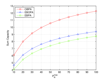
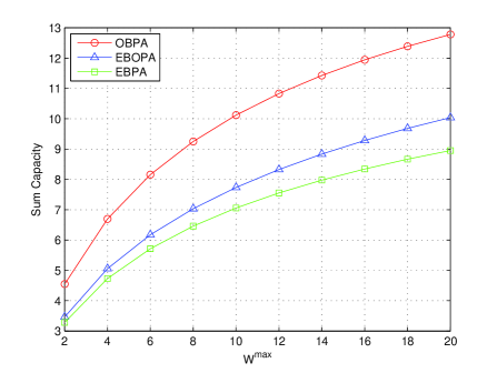
Figure 1: Sum capacity maximization based allocation: (a) $W=10$, (b) $P_{R}=40$.

In Figs. 1 (a) and (b), the performance of the sum capacity maximization based allocation is shown versus $P_{R}$ and $W$, respectively. These figures show that the OBPA scheme achieves about 30% to 50% performance improvement over the other two schemes for all parameter values. The performance improvement is higher when $P_{R}$ or $W$ is larger. The observed significant performance improvement for the OBPA can be partly attributed to the fact that the sum capacity maximization based joint bandwidth and power allocation can lead to highly unbalanced resource allocation, while bandwidth is equally allocated in the EBOPA and both bandwidth and power are equally allocated in the EBPA.

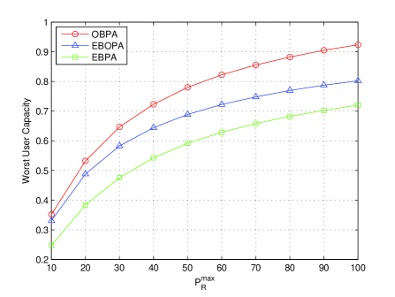
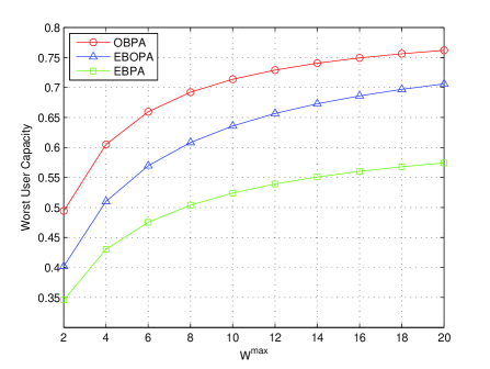
Figure 2: Worst user capacity maximization based allocation: (a) $W=10$, (b) $P_{R}=40$.

Figs. 2 (a) and (b) demonstrate the performance of the worst user capacity maximization based allocation versus $P_{R}$ and $W$, respectively. The performance improvement for the OBPA is about 10% to 30% as compared to the EBOPA for all parameter values. The improvement provided by the OBPA, in this case, is not as significant as that in Figs. 1 (a) and (b), which can be attributed to the fact that the worst user capacity maximization based allocation results in relatively balanced resource allocation, while the EBOPA and the EBPA are balanced bandwidth and totally balanced allocation schemes, respectively.

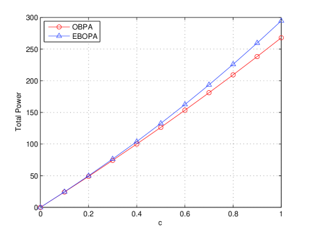
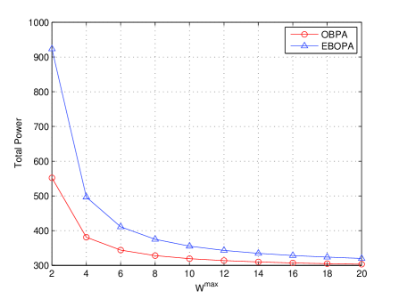
Figure 3: Power minimization based allocation: (a) $W=10$, (b) $c=1$.

Figs. 3 (a) and (b) show the total power consumption of the sources and relays versus $c$ and $W$ for the power minimization based allocation, where $c_{1}=c_{2}=c_{3}=c_{4}\triangleq c$ is assumed. Note that the total power of the OBPA is always about 10% to 30% less than that of the EBOPA, and the total power difference between the two tested schemes is larger when $c$ is larger, or when $W$ is smaller. This shows that more power is saved when the parameters are unfavorable due to the flexible bandwidth allocation in the OBPA.

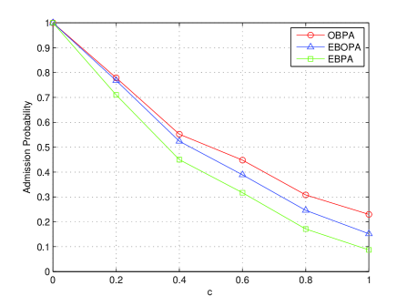
Figure 4: Admission probability vs capacity threshold.

Fig. 4 depicts the admission probability versus $c$, where $c_{1}=c_{2}=c_{3}=c_{4}\triangleq c$ is assumed. The admission probability is defined as the probability that $c$ can be satisfied for all the users under random channel realizations. The figure shows that the OBPA outperforms the other two schemes for all values of $c$, and the improvement is more significant when $c$ is large. This shows that more users or users with higher rate requirements can be admitted into the network using the OBPA scheme.

V-B Greedy Search Algorithm

In this example, the performance of the proposed greedy search algorithm is compared to that of the exhaustive search algorithm. We consider eight users $\mathcal{N}=\{1,2,\cdots,8\}$ requesting for admission. The sources and the destinations are randomly distributed inside a square area bounded by (0,0) and (10,10). We assume that $c_{i}$, $i\in\{1,2,\cdots,8\}$, is uniformly distributed over the interval $[c_{0},c_{0}+4]$ where $c_{0}$ is a variable parameter. The channel model is the same as that given in the previous subsection. We set $W=10$, $\sigma^{2}=10$ as default values. The results are averaged over 20 random channel realizations.

V-B1 Without Relaying

We consider the following two network setups.

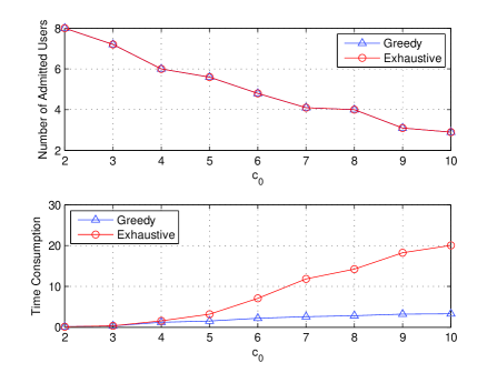
(a) setup 1

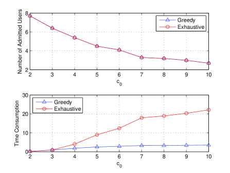
(b) setup 2

Figure 5: Greedy search algorithm vs exhaustive search algorithm.

Setup 1: In this setup, the optimality condition of the greedy search is satisfied. Specifically, there are four sources. The source assignments to the users are the following: $\mathcal{N}_{S_{1}}=\{1,2\}$, $\mathcal{N}_{S_{2}}=\{3,4\}$, $\mathcal{N}_{S_{3}}=\{5,6\}$, and $\mathcal{N}_{S_{4}}=\{7,8\}$. We set $P_{S_{i}}=40$, $\forall i\in\{1,2,3,4\}$. Fig. 5(a) shows the number of admitted users obtained by the greedy search and the corresponding computational complexity in terms of the running time versus $c_{0}$. The figure shows that the greedy search gives exactly the same number of admitted users as that of the exhaustive search for all values of $c_{0}$. This confirms that the optimal solution can be obtained when the optimality condition of the greedy search is satisfied. The time consumption of the greedy search is significantly less than that of the exhaustive search, especially when $c_{0}$ is large. This shows that the proposed algorithm is especially efficient when the number of candidate users is large and the number of admitted users is small.

Setup 2: In this setup, the optimality condition of the greedy search may not be satisfied. There are two sources and the source assignments to the users are the following: $\mathcal{N}_{S_{1}}=\{1,2,3,4\}$, and $\mathcal{N}_{S_{2}}=\{5,6,7,8\}$. We set $P_{S_{i}}=80$, $\forall i\in\{1,2\}$. Fig. 5(b) demonstrates the performance of the greedy search. Similar conclusions can be drawn for this setup as those for Setup 1. This indicates that the proposed greedy search algorithm can still perform optimally even if the sufficient optimality condition may not be satisfied.

V-B2 With Relaying

We also consider two network setups as follows.

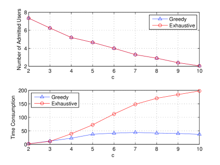
(a) setup 3

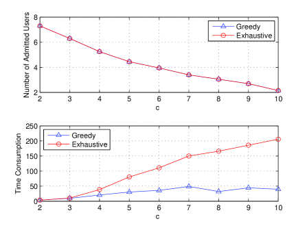
(b) setup 4

Figure 6: Greedy search algorithm vs exhaustive search algorithm.

Setup 3: In this setup, the optimality condition of the greedy search is satisfied. Specifically, in addition to the Setup 1 given in the case without relaying, four relays are included with the following user assignments: $\mathcal{N}_{R_{1}}=\{1,2\}$, $\mathcal{N}_{R_{2}}=\{3,4\}$, $\mathcal{N}_{R_{3}}=\{5,6\}$, and $\mathcal{N}_{R_{4}}=\{7,8\}$. The relays are fixed at (5,2), (5,4), (5,6), and (5,8), and we set $P_{R_{i}}=40$, $\forall i\in\{1,2,3,4\}$. Fig. 6(a) shows the number of admitted users obtained by the greedy search and the corresponding computational complexity in terms of the running time versus $c_{0}$. Similar observations can be obtained as those for Setup 1. However, it can be noted as expected that the time consumption of the greedy search for the network with relaying is much more than that for the network without relaying.

Setup 4: In this setup, the optimality condition of the greedy search may not be satisfied. Specifically, in addition to the Setup 2 given in the case without relaying, two relays are included with the following user assignments: $\mathcal{N}_{R_{1}}=\{1,2,7,8\}$, $\mathcal{N}_{R_{2}}=\{3,4,5,6\}$. The relays are fixed at (5,3) and (5,7) and we also set $P_{R_{i}}=80$, $\forall i\in\{1,2\}$. Fig. 6(b) demonstrates the performance of the greedy search. Similar conclusions can be obtained as those for Setup 3.

VI Conclusion

In this paper, joint bandwidth and power allocation has been proposed for wireless multi-user networks with and without relaying to (i) maximize the sum capacity of all users; (ii) maximize the capacity of the worst user; (iii) minimize the total power consumption of all users. It is shown that the corresponding resource allocation problems are convex and, thus, can be solved efficiently. Moreover, admission control based joint bandwidth and power allocation has been considered. Because of the high complexity of the admission control problem, a suboptimal greedy search algorithm with significantly reduced complexity has been developed. The optimality condition of the proposed greedy search has been derived and analyzed. Simulation results demonstrate the efficiency of the proposed allocation schemes and the advantages of the greedy search.

Appendix A: Proofs of Lemmas, Propositions, and Theorems in Section III

Proof of Proposition 1: We first give the following lemma.

Lemma 4: The optimal solution of the problem

$$\max_{\{p_{i},w_{i}\}}\quad\sum_{i\in\mathcal{N}}w_{i}\log\left(1+\frac{h_{i}p_{i}}{w_{i}}\right)$$ (22a)

$${\rm s.t.}\ \sum_{i\in\mathcal{N}}p_{i}\leq p$$ (22b)

$$\quad\ \ \sum_{i\in\mathcal{N}}w_{i}\leq w$$ (22c)

which is denoted by $\{p^{\ast}_{i}|i\in\mathcal{N}\}$, is $p^{\ast}_{k}=p$, $w^{\ast}_{k}=w$, and $p^{\ast}_{i}=w^{\ast}_{i}=0$, $\forall i\neq k$, where $k={\rm arg}\,\max_{i\in\mathcal{N}}h_{i}$.

Proof of Lemma 4: Consider if $\mathcal{N}=\{1,2\}$. Then the problem (22a)–(22c) is equivalent to

$$\max_{p_{1}\leq p,\;w_{1}\leq w}\quad g(w,p)=w\log\left(1+\frac{h_{1}p_{1}}{w_{1}}\right)+(w-w_{1})\log\left(1+\frac{h_{2}(p-p_{1})}{w-w_{1}}\right).$$ (23)

Assume without loss of generality that $h_{1}>h_{2}$. Consider if the constraints $0\leq p_{1}\leq p$ and $0\leq w_{1}\leq w$ are inactive at optimality. Since the problem (23) is convex, using the Karush-Kuhn-Tucker (KKT) conditions, we have

$$\log\left(1+\frac{h_{1}p^{\ast}_{1}}{w^{\ast}_{1}}\right)-\frac{h_{1}p^{\ast}_{1}}{w^{\ast}_{1}+h_{1}p^{\ast}_{1}}-\log\left(1+\frac{h_{2}(p-p^{\ast}_{1})}{w-w^{\ast}_{1}}\right)+\frac{h_{2}(p-p^{\ast}_{1})}{w-w^{\ast}_{1}+h_{2}(p-p^{\ast}_{1})}$$

$$\qquad\qquad\qquad=y\left(\frac{h_{1}p^{\ast}_{1}}{w^{\ast}_{1}}\right)-y\left(\frac{h_{2}(p-p^{\ast}_{1})}{w-w^{\ast}_{1}}\right)=0$$ (24a)

$$\frac{h_{1}w^{\ast}_{1}}{w^{\ast}_{1}+h_{1}p^{\ast}_{1}}-\frac{h_{2}(w-w^{\ast}_{1})}{w-w^{\ast}_{1}+h_{2}(p-p^{\ast}_{1})}=0.$$ (24b)

where $y(x)\triangleq\log(1+x)-x/(1+x)$. Since $y(x)$ is monotonically increasing, it can be seen from (24) that

$$\frac{h_{1}p^{\ast}_{1}}{w^{\ast}_{1}}=\frac{h_{2}(p-p^{\ast}_{1})}{w-w^{\ast}_{1}}.$$ (25)

Combining (24b) and (25), we obtain $h_{1}=h_{2}$, which contradicts the condition $h_{1}>h_{2}$. Therefore, at least one of the constraints $0\leq p_{1}\leq p$ and $0\leq w_{1}\leq w$ is active at optimality. Then it can be shown that $p^{\ast}_{1}=p$ and $w^{\ast}_{1}=w$. Note that this is also the optimal solution if $h_{1}=h_{2}$ is assumed. Furthermore, this conclusion can be directly extended to the case of $N>2$ by induction. This completes the proof. $\hfill\square$

Now we are ready to show Proposition 1. It can be seen from Lemma 1 that ${P^{\rm S}_{i}}^{\ast}={P^{\rm S}_{i}}^{\star}$, $\forall i\in\mathcal{I}$, and ${P^{\rm S}_{i}}^{\ast}=0$, $\forall i\notin\mathcal{I}$. Then the problem (4a)–(4c) is equivalent to

$$\max_{\{W^{\rm S}_{i}\}}\;\sum_{i\in\mathcal{I}}W^{\rm S}_{i}\log\left(1+\frac{{P^{\rm S}_{i}}^{\star}h^{\rm SD}_{i}}{W^{\rm S}_{i}N_{0}}\right)$$ (26a)

$${\rm s.t.}\ \sum_{i\in\mathcal{I}}W^{\rm S}_{i}\leq W.$$ (26b)

Since the problem (26a)–(26b) is convex , using the KKT conditions, we have

$$\log\left(1+\frac{{P^{\rm S}_{i}}^{\star}h^{\rm SD}_{i}}{{W^{\rm S}_{i}}^{\ast}N_{0}}\right)-\frac{{P^{\rm S}_{i}}^{\star}h^{\rm SD}_{i}}{{W^{\rm S}_{i}}^{\ast}N_{0}+{P^{\rm S}_{i}}^{\star}h^{\rm SD}_{i}}-\lambda^{\ast}=y\left(\frac{{P^{\rm S}_{i}}^{\star}h^{\rm SR}_{i}}{{W^{\rm S}_{i}}^{\ast}N_{0}}\right)-\lambda^{\ast}=0,\;i\in\mathcal{I}$$ (27a)

$$W-\sum_{i\in\mathcal{I}}{W^{\rm S}_{i}}^{\ast}=0$$ (27b)

where $\lambda^{\ast}$ denotes the optimal Lagrange multiplier, and $y(x)\triangleq\log(1+x)-x/(1+x)$. Since $y(x)$ is monotonically increasing, it follows from (27a) that

$$\frac{{P^{\rm S}_{i}}^{\star}h^{\rm SR}_{i}}{{W^{\rm S}_{i}}^{\ast}N_{0}}=\frac{{P^{\rm S}_{j}}^{\star}h^{\rm SR}_{j}}{{W^{\rm S}_{j}}^{\ast}N_{0}},\quad\forall i,j\in\mathcal{I}_{1},\ i\neq j.$$ (28)

Solving the system of equations (27b) and (28), we obtain ${W^{\rm S}_{i}}^{\ast}=Wh^{\rm SD}_{i}{P^{\rm S}_{i}}^{\star}/\sum_{j\in\mathcal{I}}h^{\rm SD}_{j}{P^{\rm S}_{j}}^{\star}$, $i\in\mathcal{I}$. This completes the proof.$\hfill\square$

Proof of Proposition 2:  It can be seen that

$$C^{\rm SD}_{i}+C^{\rm SD}_{j}=\min\{C^{\rm SR}_{i},C^{\rm RD}_{i}\}+\min\{C^{\rm SR}_{j},C^{\rm RD}_{j}\}\leq\min\{C^{\rm SR}_{i}+C^{\rm SR}_{j},C^{\rm RD}_{i}+C^{\rm RD}_{j}\}$$ (29)

When $P^{\rm S}_{j}=W^{\rm S}_{j}=P^{\rm R}_{j}=W^{\rm R}_{j}=0$, it follows from Lemma 1 that the maximum value of the right hand side of (29) is achieved and equals to $C^{\rm SD}_{i}$ and, on the other hand, the left hand side of (29) also equals to $C^{\rm SD}_{i}$. Therefore, the maximum value of $C^{\rm SD}_{i}+C^{\rm SD}_{j}$ is achieved when $P^{\rm S}_{j}=W^{\rm S}_{j}=P^{\rm R}_{j}=W^{\rm R}_{j}=0$. This completes the proof. $\hfill\square$

Appendix B: Proofs of Lemmas, Propositions, and Theorems in Section IV

Proof of Proposition 4: It is equivalent to show that there exists a feasible point $\{P^{\rm S}_{i},W^{\rm S}_{i}|i\in\mathcal{I}\}$ of the problem (12a)–(12c) if and only if $G(\mathcal{I})\leq W$. If $\{P^{\rm S}_{i},W^{\rm S}_{i}|i\in\mathcal{I}\}$ is a feasible point of the problem (12a)–(12c), then since it is also a feasible point of the problem (13a)–(13c), we have $G(\mathcal{I})\leq\sum_{i\in\mathcal{I}}W^{\rm S}_{i}\leq W$. If we have $G(\mathcal{I})\leq W$, then the optimal solution of the problem (13a)–(13c) for $\mathcal{I}$, denoted by $\{{P^{\rm S}_{i}}^{\ast},{W^{\rm S}_{i}}^{\ast}|i\in\mathcal{I}\}$, is a feasible point of the problem (12a)–(12c) since $\sum_{i\in\mathcal{I}}{W^{\rm S}_{i}}^{\ast}=G(\mathcal{I})\leq W$. This completes the proof. $\hfill\square$

Proof of Theorem 1: We first show that C1 and C2 are sufficient conditions.

Define $V(n)\triangleq G(\mathcal{N}{(t-1)})-G(\mathcal{N}{(t)})$ for $n=n{(t)}$, $1\leq t\leq N$. It follows from C2 that $V(\bar{n}_{S_{i}}{(1)})>V(\bar{n}_{S_{i}}{(2)})>\cdots>V(\bar{n}_{S_{i}}{(N_{S_{i}})})$, $\forall i\in\mathcal{M}$. Then using Proposition 2, we have $n{(t)}=\textrm{arg}\max_{n\in\mathcal{N}{(t-1)}}V(n)$, $1\leq t\leq N$. Therefore, we obtain

$$V(n{(1)})>V(n{(2)})>\cdots>V(n{(N)}).$$ (30)

It can be seen from C1 that $\mathcal{N}\setminus\mathcal{N}^{\ast}_{N-t}\cap\mathcal{N}_{S_{i}}=\textrm{arg}\min_{\mathcal{I}\subseteq\mathcal{N}_{S_{i}},|\mathcal{I}|=t_{i}}G(\mathcal{N}_{S_{i}}\setminus\mathcal{I})=\{\bar{n}_{S_{i}}{(j)}|1\leq j\leq t_{i}\}$, $\forall i\in\mathcal{M}$, where $t_{i}\triangleq|\mathcal{N}\setminus\mathcal{N}^{\ast}_{N-t}\cap\mathcal{N}_{S_{i}}|$. Then we have $\mathcal{N}\setminus\mathcal{N}^{\ast}_{N-t}=\{\bar{n}_{S_{i}}{(j)}|1\leq j\leq t_{i},i\in\mathcal{M}\}$ and $G(\mathcal{N})-G(\mathcal{N}^{\ast}_{N-t})=\sum_{i\in\mathcal{M}}\sum^{t_{i}}_{j=1}V(\bar{n}_{S_{i}}{(j)})$. Therefore, we obtain $\{t_{i}|i\in\mathcal{M}\}=\textrm{arg}\max_{\{k_{i}\};\sum_{i\in\mathcal{M}}k_{i}=t}\sum_{i\in\mathcal{M}}\sum^{k_{i}}_{j=1}V(\bar{n}_{S_{i}}{(j)})$. Since it follows from C2 that $V(\bar{n}_{S_{i}}{(1)})>V(\bar{n}_{S_{i}}{(2)})>\cdots>V(\bar{n}_{S_{i}}{(N_{S_{i}})})$, $\forall i\in\mathcal{M}$, we have $\mathcal{N}\setminus\mathcal{N}^{\ast}_{N-t}=\textrm{arg}\max_{\mathcal{I}\in\mathcal{N},|\mathcal{I}|=t}\sum_{n\in\mathcal{I}}V(n)=\{n{(i)}|1\leq i\leq t\}=\mathcal{N}\setminus\mathcal{N}{(t)}$, where the second equality is from (30). This completes the proof for sufficiency of C1 and C2.

We next show that C1 and C2 are necessary conditions by giving two instructive counter examples.

Consider if C1 does not hold. Assume without loss of generality that $\mathcal{M}=\{1\}$. Then it can be seen that C1 is equivalent to the condition (15) and, therefore, the condition (15) does not hold, either.

Consider if C2 does not hold. Assume without loss of generality that $\mathcal{M}=\{2\}$, $N_{S_{2}}=1$ and $G(\bar{\mathcal{N}}_{S_{1}}{(1)})-G(\bar{\mathcal{N}}_{S_{1}}{(2)})>G(\mathcal{N}_{S_{2}})-G(\bar{\mathcal{N}}_{S_{2}}{(1)})>G(\mathcal{N}_{S_{1}})-G(\bar{\mathcal{N}}_{S_{1}}{(1)})$. Then we have $\mathcal{N}^{\ast}_{N-2}=\mathcal{N}\setminus\{\bar{n}_{S_{1}}{(1)},\bar{n}_{S_{1}}{(2)}\}$, while it follows from Proposition 2 that $\mathcal{N}{(2)}=\mathcal{N}\setminus\{\bar{n}_{S_{1}}{(1)},\bar{n}_{S_{2}}{(1)}\}$. Therefore, $\mathcal{N}^{\ast}_{N-2}\neq\mathcal{N}{(2)}$. This completes the proof for necessity of C1 and C2. $\hfill\square$

Proof of Proposition 6: The proof of this proposition is built upon the following two lemmas. It suffices to show that C2 holds for $i=1$.

Lemma 5: If $p_{1}>p_{2}>\Delta p>0$, the following inequality holds

$$F_{i}(p_{1}-\Delta p)-F_{i}(p_{1})<F_{i}(p_{2}-\Delta p)-F_{i}(p_{1}).$$ (31)

Proof of Lemma 5: It can be shown that $F_{i}(p)$ is a strictly convex and decreasing function of $p$. Using the first order convexity condition, we have

$$F_{i}(p_{2}-\Delta p)-F_{i}(p_{2})>-F^{\prime}_{i}(p_{2})\Delta p$$ (32)

and

$$F_{i}(p_{1}-\Delta p)-F_{i}(p_{1})<-F^{\prime}_{i}(p_{1}-\Delta p)\Delta p$$ (33)

where $F^{\prime}_{i}$ is the first order derivative of $F_{i}$. Consider two cases. (i) If $p_{2}\leq p_{1}-\Delta p$, then $F^{\prime}_{i}(p_{2})\leq F^{\prime}_{i}(p_{1}-\Delta p)$ due to the convexity of $F_{i}(p_{2})$. Therefore, using $\Delta p>0$ together with (32) and (33), we obtain (31); (ii) If $p_{2}\geq p_{1}-\Delta p$, using $p_{1}>p_{2}$ and a similar argument as in 1), we can show that $F_{i}(p_{2})-F_{i}(p_{1})<F_{i}(p_{2}-\Delta p)-F_{i}(p_{1}-\Delta p)$, which is equivalent to (31). This completes the proof. $\hfill\square$

$G(\mathcal{N}_{S_{1}})$ can be extended to $G(\mathcal{N}_{S_{1}},P_{S_{1}})$ if $P_{S_{1}}$ is considered as a variable.

Lemma 6: $p^{\ast}_{i}$, $\forall i\in\mathcal{N}_{S_{1}}$, is increasing with $P_{S_{1}}$, where $\{p^{\ast}_{i}|i\in\mathcal{N}_{S_{1}}\}$ denotes the optimal solution of the problem (17a)–(17b) for $\mathcal{N}_{S_{1}}$ and $P_{S_{1}}$.

Proof of Lemma 6: The inverse function of $w=F_{i}(p)$ is $p=F^{-1}_{i}(w)=(e^{c_{i}/w}-1)w/h_{i}$. Then we have

$$G(\mathcal{N}_{S_{1}},P_{S_{1}})=\max_{w_{i}}\sum_{i\in\mathcal{N}_{S_{1}}}w_{i}$$ (34a)

$$\textrm{s.t.}\ \sum_{i\in\mathcal{N}_{S_{1}}}F^{-1}_{i}(w_{i})\leq P_{S_{1}}.$$ (34b)

Since the problem (34b)–(34b) is convex, using the KKT conditions, the optimal solution and the optimal Lagrange multiplier of this problem, denoted by $\{w^{\ast}_{i}|i\in\mathcal{N}_{S_{1}}\}$ and $\lambda^{\ast}$, respectively, satisfy the following equations

$$1+\frac{\lambda^{\ast}}{h_{i}}\left(e^{\frac{c_{i}}{w_{i}^{\ast}}}\left(\frac{c_{i}}{w_{i}^{\ast}}-1\right)+1\right)=0,\quad\forall i\in\mathcal{N}_{S_{1}}.$$ (35)

It can be shown that $(e^{c_{i}/w_{i}^{\ast}}(c_{i}/w_{i}^{\ast}-1)+1)/h_{i}$ is monotonically decreasing with $w_{i}^{\ast}$. Therefore, $w^{\ast}_{i}$, $\forall i\in\mathcal{N}_{S_{1}}$, and, correspondingly, $p^{\ast}_{i}=F^{-1}_{i}(w^{\ast}_{i})$, $\forall i\in\mathcal{N}_{S_{1}}$, is decreasing and increasing, respectively, with $\lambda^{\ast}$. Then it follows from (34b) that $p^{\ast}_{i}$, $\forall i\in\mathcal{N}_{S_{1}}$, is increasing with $P_{S_{1}}$. This completes the proof. $\hfill\square$

We are now ready to prove this proposition. Let $P_{1}>P_{2}$ and $\mathcal{N}^{-k}_{S_{1}}\triangleq\mathcal{N}_{S_{1}}\setminus\{k\}$ for some $k\in\mathcal{N}_{S_{1}}$. Let $\{p^{\star}_{i}|i\in\mathcal{N}^{-k}_{S_{1}}\}$ denote the optimal solution of the problem (17a)–(17b) for $\mathcal{N}^{-k}_{S_{1}}$ and $P_{2}$. Using Lemma 6, the optimal solution of the problem (17a)–(17b) for $G(\mathcal{N}_{S_{1}},P_{2})$ can be expressed as $\{p^{\star}_{i}-\Delta p_{i}\}$, $i\in\mathcal{N}^{-k}_{S_{1}}$, and $p^{\star}_{k}$, respectively, where $\Delta p_{i}>0$ and $\sum_{i\in\mathcal{N}^{-k}_{S_{1}}}\Delta p_{i}=p^{\star}_{k}$. Then we have

$$G(\mathcal{N}_{S_{1}},P_{2})-G(\mathcal{N}^{-k}_{S_{1}},P_{2})=\sum_{i\in\mathcal{N}^{-k}_{S_{1}}}\left(F_{i}(p^{\star}_{i}-\Delta p_{i})-F_{i}(p^{\star}_{i})\right)+F_{k}(p^{\star}_{k}).$$ (36)

Let $\{p^{+}_{i}|i\in\mathcal{N}^{-k}_{S_{1}}\}$ denote the optimal solution of the problem (17a)–(17b) for $\mathcal{N}^{-k}_{S_{1}}$ and $P_{1}$. Then we have

$$G(\mathcal{N}_{S_{1}},P_{1})-G(\mathcal{N}^{-k}_{S_{1}},P_{1})\!\!\!\! = \!\!\!\!\min_{\{p_{i}\};\sum_{i\in\mathcal{N}_{S_{1}}}p_{i}\leq P_{1}}\sum_{i\in\mathcal{N}_{S_{1}}}F_{i}(p_{i})-\sum_{i\in\mathcal{N}^{-k}_{S_{1}}}F_{i}(p^{+}_{i})$$ (37)

$$\leq \!\!\!\!\sum_{i\in\mathcal{N}^{-k}_{S_{1}}}(F_{i}(p^{+}_{i}-\Delta p_{i})-F_{i}(p^{+}_{i}))+F_{k}(p^{\star}_{k}).$$

Since $P_{1}>P_{2}$, it follows from Lemma 6 that $p^{+}_{i}>p^{\star}_{i}>\Delta p_{i}>0$, $i\in\mathcal{N}^{-k}_{S_{1}}$. Using Lemma 5, we obtain $F_{i}(p^{+}_{i}-\Delta p_{i})-F_{i}(p^{+}_{i})<F_{i}(p^{\star}_{i}-\Delta p_{i})-F_{i}(p^{\star}_{i})$, $j\in\mathcal{N}^{-k}_{S_{1}}$. Therefore, comparing (36) with (37), we have

$$G(\mathcal{N}_{S_{1}},P_{1})-G(\mathcal{N}^{-k}_{S_{1}},P_{1})<G(\mathcal{N}_{S_{1}},P_{2})-G(\mathcal{N}^{-k}_{S_{1}},P_{2}).$$ (38)

which can be rewritten as

$$G(\mathcal{N}^{-k}_{S_{1}},P_{2})-G(\mathcal{N}^{-k}_{S_{1}},P_{1})<G(\mathcal{N}_{S_{1}},P_{2})-G(\mathcal{N}_{S_{1}},P_{1}).$$ (39)

Let $\{p^{\ast}_{i}|i\in\mathcal{N}_{S_{1}}\}$, denote the optimal solution of the problem (17a)–(17b) for $\mathcal{N}_{S_{1}}$ and $P_{S_{1}}$. Then we have

$$G(\mathcal{N}_{S_{1}}\!\setminus\!\{\bar{n}_{S_{1}}{(2)}\},P_{S_{1}})\!-\!G(\bar{\mathcal{N}}_{S_{1}}{(2)},P_{S_{1}})\!\!\!\! \leq \!\!\!\!F_{\bar{n}_{S_{1}}{(1)}}(p^{\ast}_{\bar{n}_{S_{1}}{(1)}})\!+\!G(\bar{\mathcal{N}}_{S_{1}}{(2)},P_{S_{1}}\!-\!p^{\ast}_{\bar{n}_{S_{1}}{(1)}})\!-\!G(\bar{\mathcal{N}}_{S_{1}}{(2)},P_{S_{1}})$$ (40)

$$< \!\!\!\!F_{\bar{n}_{S_{1}}{(1)}}(p^{\ast}_{\bar{n}_{S_{1}}{(1)}})\!+\!G(\bar{\mathcal{N}}_{S_{1}}{(1)},P_{S_{1}}\!-\!p^{\ast}_{\bar{n}_{S_{1}}{(1)}})\!-\!G(\bar{\mathcal{N}}_{S_{1}}{(1)},P_{S_{1}})$$

$$= \!\!\!\!G(\mathcal{N}_{S_{1}},P_{S_{1}})-G(\bar{\mathcal{N}}_{S_{1}}{(1)},P_{S_{1}})$$

where the second inequality follows from (39). On the other hand, we have

$$\begin{split}G(\mathcal{N}_{S_{1}}\setminus\{\bar{n}_{S_{1}}{(2)}\},P_{S_{1}})-G(\bar{\mathcal{N}}_{S_{1}}{(2)},P_{S_{1}})&\geq G(\mathcal{N}_{S_{1}}\setminus\{\bar{n}_{S_{1}}{(1)}\},P_{S_{1}})-G(\bar{\mathcal{N}}_{S_{1}}{(2)},P_{S_{1}})\\ &=G(\bar{\mathcal{N}}_{S_{1}}{(1)},P_{S_{1}})-G(\bar{\mathcal{N}}_{S_{1}}{(2)},P_{S_{1}}).\end{split}$$ (41)

Therefore, comparing (40) with (41), we completes the proof. $\hfill\square$

Proof of Lemma 2: Assume $\mathcal{N}_{S_{l},k}\neq\mathcal{N}^{\ast}_{S_{l},k}$. Then there exist $a\in\mathcal{N}^{\ast}_{S_{l},k}$ and $b\in\mathcal{N}\setminus\mathcal{N}^{\ast}_{S_{l},k}$ such that $F_{a}(p)>F_{b}(p)$. Let $\{p^{\ast}_{i}|i\in\mathcal{N}^{\ast}_{S_{1},k}\}$ denote the optimal solution of the problem (17a)–(17b) for $G(\mathcal{N}^{\ast}_{S_{l},k})$. Then there always exists $\mathcal{N}^{\prime}_{S_{l},k}\triangleq\mathcal{N}^{\ast}_{S_{l},k}\cup\{b\}\setminus\{a\}$ such that

$$\begin{split}G(\mathcal{N}^{\ast}_{S_{l},k})&=\sum_{i\in\mathcal{N}^{\ast}_{S_{l},k},\;i\neq a}F_{i}(p^{\ast}_{i})+F_{a}(p^{\ast}_{a})>\sum_{i\in\mathcal{N}^{\ast}_{S_{l},k},\;i\neq a}F_{i}(p^{\ast}_{i})+F_{b}(p^{\ast}_{a})\\ &\geq\min_{\{p_{i}\};\;\sum_{i\in\mathcal{N}^{\prime}_{S_{l},k}}p_{i}\leq P_{S_{1}}}\sum_{i\in\mathcal{N}^{\prime}_{S_{l},k}}F_{i}(p_{i})=G(\mathcal{N}^{\prime}_{S_{l},k})\end{split}$$ (42)

which contradicts the definition of $\mathcal{N}^{\ast}_{S_{l},k}$. Then it follows that $\mathcal{N}_{S_{l},k}=\mathcal{N}^{\ast}_{S_{l},k}$. Using similar arguments, it can be shown that $\mathcal{N}_{S_{l},k}=\bar{\mathcal{N}}_{N_{S_{l}}}{(N_{S_{l}}-k)}$. This completes the proof. $\hfill\square$

Proof of Proposition 7: It suffices to show that C1 holds for $i=1$ if for any $j\in\mathcal{N}_{S_{1}}$, there exists no more than one $k\in\mathcal{N}_{S_{1}}$, $k\neq j$, such that C3 holds. It can be seen that for any $1\leq k\leq N_{S_{1}}$, only two cases are under consideration: (i) there exists $\mathcal{N}_{S_{1},k}$ that satisfies the condition given in Lemma 4 and, therefore, $\mathcal{N}^{\ast}_{S_{1},k}=\mathcal{N}{(N_{S_{1}}-k)}$; (ii) there exist $\mathcal{N}_{S_{1},k-1}$ and $\mathcal{N}_{S_{1},k+1}$ that satisfy the condition given in Lemma 2 respectively and, therefore, $\mathcal{N}^{\ast}_{S_{1},k-1}=\mathcal{N}{(N_{S_{1}}-k+1)}\subseteq\mathcal{N}{(N_{S_{1}}-k-1)}=\mathcal{N}^{\ast}_{S_{1},k+1}$. Then it follows that $\mathcal{N}^{\ast}_{S_{1},k}=\mathcal{N}{(N_{S_{1}}-k)}$. This completes the proof. $\hfill\square$

Proof of Lemma 3: Consider if $F_{i}(p)$ intersects $F_{j}(p)$ at a point $(p^{\prime},w^{\prime})$. Then we obtain

$$\frac{c_{j}}{c_{i}}=\frac{w^{\prime}\log\left(1+\frac{h_{j}p^{\prime}}{w^{\prime}}\right)}{w^{\prime}\log\left(1+\frac{h_{i}p^{\prime}}{w^{\prime}}\right)}=q\left(\frac{p^{\prime}}{w^{\prime}}\right)$$ (43)

where $q(x)=\log(1+h_{j}x)/\log(1+h_{i}x)$, $0<x<\infty$. It can be shown that $\underset{x\rightarrow 0}{\lim}q(x)=h_{j}/h_{i}$, $\underset{x\rightarrow\infty}{\lim}q(x)=1$, and $q(x)$ is monotonically decreasing with $x$. Therefore, the range of $q(x)$ is $(1,h_{j}/h_{i})$. If $c_{j}/c_{i}\in(1,h_{j}/h_{i})$, there exists a unique solution $x^{\prime}$ such that $q(x^{\prime})=c_{j}/c_{i}$. Hence, $F_{i}(p)$ and $F_{j}(p)$ have a unique intersection point given by $w^{\prime}=c_{j}/\log(1+h_{j}x^{\prime})$, $p^{\prime}=w^{\prime}x^{\prime}$, and the claim (i) follows. If $c_{j}/c_{i}\notin(1,h_{j}/h_{i})$, there is a special case that $F_{i}(p)=F_{j}(p)$, $\forall p>0$ if $h_{j}/h_{i}=c_{j}/c_{i}=1$. Otherwise, the solution of (43) does not exist, i.e., $F_{i}(p)$ does not intersect $F_{j}(p)$ and, therefore, the claims (ii) and (iii) also follow. This completes the proof. $\hfill\square$

References

- [1] D. Julian, M. Chiang, D. O’Neill, and S. Boyd, “QoS and fairness constrained convex optimization of resource allocation for wireless cellular and ad hoc networks,” in Proc. IEEE Infocom, New York, Jun. 2002, pp. 477-486.
- [2] L. Xiao, M. Johansson and S. Boyd, “Simultaneous routing and resource allocation via dual decomposition,” IEEE Trans. Commun., vol. 52, pp. 1136-1144, Jul. 2004.
- [3] R. D. Yates, “A framework for uplink power control in cellular radio systems,” IEEE J. Select. Areas Commun., vol. 13, pp. 1341-1347, Sept. 1995.
- [4] F. Rashid-Farrokhi, K. J. R. Liu, and L. Tassiulas, “Transmit beamforming and power control for cellular wireless systems,” IEEE J. Select. Areas Commun., vol. 16, pp. 1437-1450, Oct. 1998.
- [5] M. Chiang, “Geometric programming for communication systems” Foundations and Trends in Communications and Information Theory, vol. 2, no. 1-2, pp. 1-154, Aug. 2005.
- [6] K. Kumaran and H. Viswanathan, “Joint power and bandwidth allocation in downlink transmission,” IEEE Trans. Wireless Commun., vol. 4, pp. 1008-1016, May. 2005.
- [7] J. Acharya and R. D. Yates, “Dynamic spectrum allocation for uplink users with heterogeneous utilities,” IEEE Trans. Wireless Commun., vol. 8, pp. 1405-1413, Mar. 2009.
- [8] I. Maric and R. D. Yates, “Bandwidth and power allocation for cooperative strategies in gaussian relay networks”, IEEE Trans. Inform. Theory, vol. 56, pp. 1880-1889, Apr. 2010.
- [9] J. Laneman, D. Tse, and G. Wornell, “Cooperative diversity in wireless networks: efficient protocols and outage behavior,” IEEE Trans. Inform. Theory, vol. 50, pp. 3062-3080, Dec. 2004.
- [10] G. Kramer, M. Gastpar, and P. Gupta, “Cooperative strategies and capacity theorems for relay networks”, IEEE Trans. Inform. Theory, vol. 51, pp. 3037-3063, Sep. 2005.
- [11] Y.-W. Hong, W.-J. Huang, F.-H. Chiu, and C.-C. J. Kuo, “Cooperative communications in resource-constrained wireless networks,” IEEE Signal Process. Mag., vol. 24, pp. 47-57, May 2007.
- [12] J. Luo, R. S. Blum, L. J. Cimini, L. J. Greenstein, and A. M. Haimovich, “Decode-and-forward cooperative diversity with power allocation in wireless networks,” IEEE Trans. Wireless Commun., vol. 6, pp. 793-799, Mar 2007.
- [13] V. Havary-Nassab, S. Shahbazpanahi, and A. Grami, “Optimal distributed beamforming for two-way relay networks,” IEEE Trans. Signal Process., vol. 58, pp. 1238-1250, Mar. 2010.
- [14] L. Xie and X. Zhang, “TDMA and FDMA based resource allocations for quality of service provisioning over wireless relay networks,” in Proc. IEEE Wireless Commun. and Networking Conf., Hong Kong, Mar. 2007, pp. 3153-3157.
- [15] S. Senthuran, A. Anpalagan, and O. Das, “Cooperative subcarrier and power allocation for a two-hop decode-and-forward OFCMD based relay network ,” IEEE Trans. Wireless Commun., vol. 6, pp. 4797-4805 , Sep. 2009.
- [16] A. Y. Panah, R. W. Heath, “Single-user and multicast OFDM power loading with nonregenerative relaying,” IEEE Trans. Veh. Technol., vol. 58, pp. 4890-4902, Nov. 2009.
- [17] S. Serbetli and A. Yener, “Relay assisted F/TDMA ad hoc networks: node classification, power allocation and relaying strategies,” IEEE Trans. Commun., vol. 56, pp. 937-947, Jun. 2008.
- [18] K. T. Phan, T. Le-Ngoc, S. A. Vorobyov, and C. Tellambura, “Power allocation in wireless multi-user relay networks,” IEEE Trans. Wireless Commun., vol. 8, pp. 2535-2545, May. 2009.
- [19] K. T. Phan, L. B. Le, S. A. Vorobyov, and T. Le-Ngoc, “Power allocation and admission control in multiuser relay networks via convex programming: centralized and distributed schemes,” EURASIP Journal on Wireless Communications and Networking, vol. 2009, 2009, Article ID 901965.
- [20] E. Matskani, N. D. Sidiropoulos, Z.-Q. Luo, and L. Tassiulas, “Convex approximation techniques for joint multiuser downlink beamforming and admission control,” IEEE Trans. Wireless Commun., vol. 7, pp. 2682-2693, Jul. 2008.
- [21] E. Matskani, N. D. Sidiropoulos, Z.-Q. Luo, and L. Tassiulas, “Efficient batch and adaptive approximation algorithms for joint multicast beamforming and admission control,” IEEE Trans. Signal Processing, vol. 57, pp. 4882-4894, Dec. 2009.
- [22] L. B. Le and E. Hossain, “Resource allocation for spectrum underlay in cognitive radio networks,” IEEE Trans. Wireless Commun., vol. 7, pp. 5306-5315, Dec. 2008.
- [23] M. Andersin, Z. Rosberg, and J. Zander, “Gradual removals in cellular PCS with constrained power control and noise,” ACM Wireless Networks J., vol. 2, pp. 27-43, 1996.
- [24] X. Gong, S. A. Vorobyov, and C. Tellambura, “Joint bandwidth and power allocation in multi-user decode-and-forward relay networks,” in Proc. 35th IEEE Inter. Conf. Acoustics, Speech, and Signal Processing, Dallas, Texas, USA, Mar. 2010, pp. 2498-2501.
- [25] S. Gault, W. Hachem, and P. Ciblat, “Performance analysis of an OFDMA transmission system in a multicell environment,” IEEE Trans. Commun., vol. 55, pp. 740 - 751, Apr. 2007.
- [26] S. Boyd and L. Vandenberghe. Convex Optimization. Cambridge University Press, 2004.
- [27] TOMLAB Optimization Environment, http://tomopt.com/