Conjecture concerning a completely monotonic function

Abstract

Based on a sequence of numerical computations, a conjecture is presented regarding the class of functions $H(x;a)=\exp(a)-(1+a/x)^{x}$, and the open problem of determining the values of $a$ for which the functions are completely monotonic with respect to $x$. The critical value of $a$ is determined here to sufficient accuracy to show that it is not a simple symbolic quantity.

1 Introduction

A completely monotonic (CM) function is an infinitely differentiable function $f:(0,\infty)\to\mathbb{R}$ whose derivatives satisfy

$$\forall x>0,\forall n\in\mathbb{N},(-1)^{n}f^{(n)}(x)\geq 0\ .$$

The definition is due to Hausdorff [4], and a collection of important properties can be found in [7]. Alzer and Berg [1] state the following open problem. Consider the function

$$H(x;a)=e^{a}-\left(1+\frac{a}{x}\right)^{x}\ .$$ (1)

For what values of the parameter $a$ is $H(x;a)$ completely monotonic (CM)?

A problem that is superficially similar to this problem has a remarkably simple solution [1]. The function

$$J(x;a,b)=\left(1+\frac{a}{x}\right)^{x+b}-e^{a}$$ (2)

is CM if and only if $a\leq 2b$. Although $H(x;a)=-J(x;a,0)$, the problems for $J$ and $H$ are essentially different, because a completely monotonic function must be positive and decreasing. A more completely descriptive name might be ‘completely monotonically decreasing function’, but the shorter name is now standard. In spite of the beautiful result for $J$, a consequence of the conjecture advanced here is that no similarly simple result applies to $H(x;a)$.

Alzer and Berg [1] show that $H(x;1)$ is CM. Moreover, Berg [3] has shown, through an equivalent problem, that $H(x;3)$ is not CM. Therefore, it has been conjectured that there exists a value $a_{\mathrm{c}}$ such that $H(x;a)$ is completely monotonic for all $a<a_{\mathrm{c}}$ and not for $a>a_{\mathrm{c}}$. We obtain here experimentally an estimate for its value, namely $a_{\mathrm{c}}\approx 2.299656443$.

In the field of experimental mathematics, there are several tools for identifying a real number with an expression containing known mathematical constants. We have applied these tools to $a_{\mathrm{c}}$, but without success.

2 Heuristic description of method

In this section we give a graphical and heuristic description of the method we use. For convenience, we define the function

$$f(x,a,n)=(-1)^{n}\frac{\partial^{n}}{\partial x^{n}}H(x;a)\ ,$$ (3)

and consider its properties for various fixed $n$.

We start with the case $n=2$. Figure 1(a) shows plots of $f(x,a,2)$, or equivalently the second derivative of $H$. For $a=2.9$, the function is clearly monotonic decreasing; for $a=3.4$, the function is clearly not monotonic. The transition occurs for $a=a_{\mathrm{f}}\approx 3.138$, when $f(x,a_{\mathrm{f}},2)$ has an inflexion point at $x=x_{\mathrm{f}}\approx 0.913$, as shown.

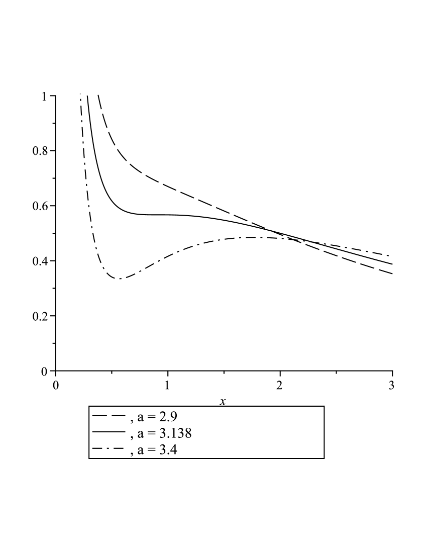
(a) (b)

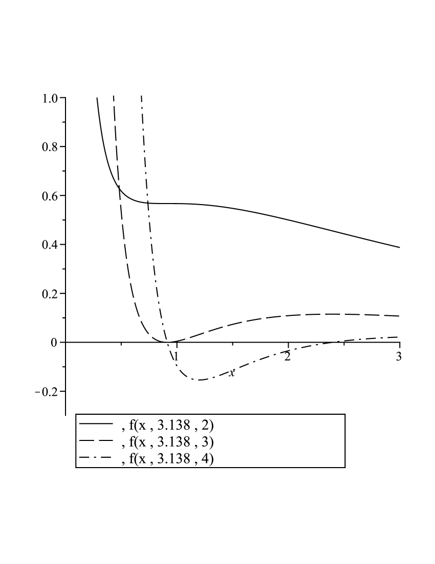
Figure 1: (a) $f(x,a,2)$ for three values of $a$. The function $f(x,2.9,2)$ is monotonic, $f(x,3.4,2)$ is not monotonic, and $f(x,3.138,2)$ is the transitional case for $n=2$. (b) The right plot shows for the critical value $a=3.138$ the successive derivatives $f(x,3.138,2)$, $f(x,3.138,3)$ and $f(x,3.138,4)$.

The transitional case is further considered in figure 1(b), where the second, third and fourth derivatives are plotted. As could be anticipated from the shape of $f(x,a_{\mathrm{f}},2)$, its derivative $f(x,a_{\mathrm{f}},3)$ touches the $x$-axis at $x=x_{\mathrm{f}}$. Further, $f(x,a_{\mathrm{f}},4)$ crosses the axis at the same point. From these observations, it is obvious that the pair of values $a_{\mathrm{f}},x_{\mathrm{f}}$ satisfy the equations

$$f(x_{\mathrm{f}},a_{\mathrm{f}},3) = 0\ ,$$ (4)

$$f(x_{\mathrm{f}},a_{\mathrm{f}},4) = 0\ .$$ (5)

Now consider the case $n=3$. The above series of observations can be repeated for $f(x,a,3)$. Again there is a range of values of $a$ for which the function is monotonic decreasing, and there is a critical pair $a_{\mathrm{f}},x_{\mathrm{f}}$ such that $f(x_{\mathrm{f}},a_{\mathrm{f}},3)$ is an inflexion point. Solving the pair of equations $f(x_{\mathrm{f}},a_{\mathrm{f}},4)=f(x_{\mathrm{f}},a_{\mathrm{f}},5)=0$ gives $a_{\mathrm{f}}\approx 2.903$, $x_{\mathrm{f}}\approx 1.344$. In general, the function $f(x,a,n)$ will be monotonic decreasing for $a$ ‘small enough’. From Alzer and Berg [1], $a=1$ is always such a value. The change to non-monotonic behaviour will occur at a value $a_{\mathrm{f}}(n)$ when $f(x,a,n)$ has an inflexion point at $x_{\mathrm{f}}(n)$. The values of $a_{\mathrm{f}}(n)$ and $x_{\mathrm{f}}(n)$ can be determined from the equations

$$f(x_{\mathrm{f}},a_{\mathrm{f}},n+1)=f(x_{\mathrm{f}},a_{\mathrm{f}},n+2)=0\ .$$

We next consider how $a_{\mathrm{f}}(n)$ depends upon $n$. We have seen already that $a_{\mathrm{f}}(2)\approx 3.138$, and $a_{\mathrm{f}}(3)\approx 2.903$. For all $n>2$, $a_{\mathrm{f}}(n+1)<a_{\mathrm{f}}(n)$. This is so because if $f(x,a_{\mathrm{f}}(n),n)$ has an inflexion point, then $f(x,a_{\mathrm{f}}(n),n+1)$ must be non-monotonic. Therefore, if one thinks of $a$ as increasing from $a=1$, for which value all functions are monotonic, then $f(x,a,n+1)$ must have become non-monotonic at a lower value of $a$ than that for which $f(x,a,n)$ becomes non-monotonic. Thus the sequence $\{a_{\mathrm{f}}(n)\}$ must be monotonically decreasing and it is bounded below by $1$ from the results in [1]. Therefore the limit $a_{\mathrm{c}}=\lim_{n\to\infty}a_{\mathrm{f}}(n)$ exists and is the critical value of $a$ such that $H(x;a)$ is completely monotonic for $a<a_{\mathrm{c}}$.

3 Numerical method

In view of the above observations, we need to compute $a_{\mathrm{f}}(n)$ for a selection of values of $n$ and then extrapolate to compute the limit $n\to\infty$. In order to obtain a value of $a_{\mathrm{c}}$ that is accurate enough to be submitted to tools such as Plouffe’s inverter [5], we need to compute derivatives up to the order of $10^{5}$. Hence, an efficient method must be found to evaluate $f(x,a,n)$ for large values of $n$. Symbolic differentiation becomes impossible after at most $n=50$, depending upon the memory available on the computer used, implying the need for a numerical scheme.

By introducing the notation

$$h=\left(1+\frac{a}{x}\right)^{x}\ ,$$

we can write $H(x;a)=\exp(a)-h$, and obtain

$$f(x,a,0) = H(x;a)=e^{a}-h\ ,$$ (6)

$$f(x,a,1) = \frac{\partial h}{\partial x}=\left(\ln\frac{x+a}{x}-\frac{a}{x+a}\right)h\ .$$ (7)

Leibnitz’s rule now allows us to compute recursively.

$$f(x,a,n) = (-1)^{n-1}\frac{\partial^{n-1}}{\partial x^{n-1}}f(x,a,1)$$ (8)

$$= (-1)^{n-1}\sum_{k=0}^{n-1}\binom{n-1}{k}\frac{\partial^{k}h}{\partial x^{k}}\frac{\partial^{n-1-k}}{\partial x^{n-1-k}}\left(\ln\frac{x+a}{x}-\frac{a}{x+a}\right).$$

The second term in the sum can be computed explicitly by introducing the following function.

$$g(x,a,n)=\begin{cases}-\ln\frac{x+a}{x}+\frac{a}{x+a}\ ,&n=0\ ,\\ -\frac{(n-1)!}{x^{n}}+\frac{(n-1)!}{(x+a)^{n}}+\frac{n!a}{(x+a)^{n+1}}\ ,&n\geq 1.\end{cases}$$

Thus the computational form of (8) becomes

$$f(x,a,n)=\sum_{k=0}^{n-1}\binom{n-1}{k}f(x,a,k)g(x,a,n-1-k)\ .$$ (9)

Although it is possible to compute with this formula symbolically, expression swell prevents this approach from being useful for anything other than for error checking. If we assign numerical values to $x$ and $a$ and compute $f(x,a,0)$ numerically, then (9) can evaluate derivatives numerically to orders $10^{6}$ or more.

Once the functions $f(x,a,n)$ can be computed efficiently, the equations $f(x_{\mathrm{f}},a_{\mathrm{f}},n+1)=0$, $f(x_{\mathrm{f}},a_{\mathrm{f}},n+2)=0$ can be solved to find the transition point in $f(x,a,n)$. For small values of $n$, any method, for example Maple’s fsolve, can be used. For large $n$, extended precision must be used, owing to loss of precision through the accumulaton of cancellation and rounding errors. For $n$ greater than $10^{4}$ the precision loss amounts to about 15 decimal digits. The equations were solved using bivariate Newton iteration. The required derivatives with respect to $a$ can be computed using a method analogous to that above. In addition to cancelation errors, there is another reason for requiring extended precision. Because $(x_{\mathrm{f}},a_{\mathrm{f}})$ is a repeated root of $f(x_{\mathrm{f}},a_{\mathrm{f}},n+1)$, Newton iteration converges slowly and a nearly singular matrix must be inverted. Therefore 60 decimal digits were used in the computations. For smaller $n$, Maple was used, but became too slow for larger $n$, and Bailey’s ARPREC [2] and Gnu GMP were used.

4 Results

Table 1 displays critical values computed between $n=1000$ and $n=100000$. Each entry gives the smallest value of $a$ such that $f(x_{\mathrm{f}},a,n+1)<0$. That is, for each entry, $f(x_{\mathrm{f}},a_{\mathrm{f}}-10^{-14},n+1)>0$.

n	$a_{\mathrm{f}}(n)$	$x_{\mathrm{f}}(n)$
1000	2.30183958971854	436.380167908055
2000	2.30074838075010	872.743540008136
4000	2.30020250313093	1745.47034071250
5000	2.30009330574014	2181.83374672043
10000	2.29987488908353	4363.65078807689
12500	2.29983120225165	5454.55931101894
16000	2.29979297531646	6981.83124393025
20000	2.29976566981568	8727.28488210931
40000	2.29971105744643	17454.5530758350
50000	2.29970013475374	21818.1871732641
100000	2.29967828914950	43636.3576615316

Table 1: Table of critical values.

To extrapolate to $n\to\infty$, we examine $a_{\mathrm{f}}$ as a function of $n^{-1}$. Figure 2 shows a plot of $a_{\mathrm{f}}(n)$ against $n^{-1}$. We conjecture that $a_{\mathrm{f}}$ obeys a relation

$$a_{\mathrm{f}}=a_{\mathrm{c}}+\frac{a_{1}}{n}+\frac{a_{2}}{n^{2}}+O(n^{-3}).$$ (10)

By fitting a quadratic in $n^{-1}$ using the data points $n=40000,\,50000,\,100000$, we obtain $a_{\mathrm{c}}\approx 2.29965644325$, where the error can be expected to be $O(10^{-12})$. This value was given to Plouffe’s inverter [5], the inverse symbolic calculator [6], and Maple’s identify command. No symbolic quantity matched all digits, and the closest symbolic quantities offered no immediate inspiration for analytic investigations.

5 Closing remarks

The simple solution to problem (2) has led to several attempts to find an equally simple solution for (1). The numerical evidence presented suggests that such attempts will continue to fail. The numerical data obtained here does, however, suggest a number of simple properties which might help in an analytical solution to the problem. The dependence of $x_{\mathrm{f}}(n)$ on $n$ suggests a strongly linear correlation between $x_{\mathrm{f}}$ and $n$. A similar correlation between $a_{\mathrm{c}}(n)$ and $n^{-1}$ has been noted above. If these numerical observations can be explained analytically, then a full solution might follow.

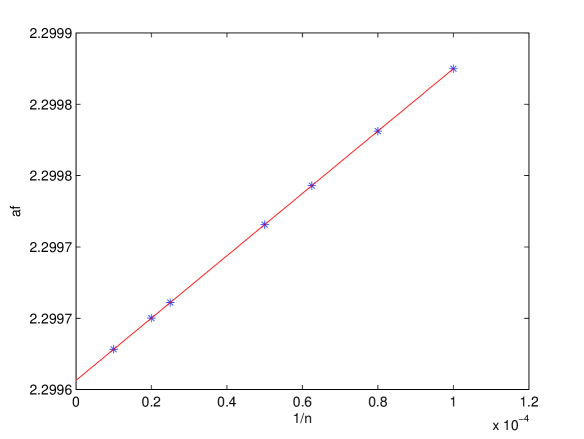
Figure 2: A plot of $a_{\mathrm{f}}$ against $n^{-1}$.

References

- [1] Alzer, H. and Berg, C., Some classes of completely monotonic functions, Annales Academiæ Scientiarum Fennicæ Mathematica, 27, 445–460, 2002.
- [2] http://crd.lbl.gov/~dhbailey/mpdist/
- [3] Berg, C., Problem 1. Bernstein functions, J. Comput. Appl. Math., 178, 525–526, 2005.
- [4] Hausdorff, F., Summationsmethoden und Momentfolgen I. Math. Z. 9, 74–109, 1921.
- [5] http://pi.lacim.uqam.ca/eng/.
- [6] http://oldweb.cecm.sfu.ca/projects/ISC/ISCmain.html
- [7] Widder, D.V., The Laplace Transform. Princeton Univ. Press, Princeton, NJ, 1941.