Higher order moment models of dense stellar systems:
Applications to the modeling of the stellar velocity distribution function

Abstract

Dense stellar systems such as globular clusters, galactic nuclei and nuclear star clusters are ideal loci to study stellar dynamics due to the very high densities reached, usually a million times higher than in the solar neighborhood; they are unique laboratories to study processes related to relaxation. There are a number of different techniques to model the global evolution of such a system. We can roughly separate these approaches into two major groups; the particle-based models, such as direct $N-$body and Monte Carlo models, and the statistical models, in which we describe a system of a very large number of stars through a one-particle phase space distribution function. In this approach we assume that relaxation is the result of a large number of two-body gravitational encounters with a net local effect. We present two moment models that are based on the collisional Boltzmann equation. By taking moments of the Boltzmann equation one obtains an infinite set of differential moment equations where the equation for the moment of order $n$ contains moments of order $n+1$. In our models we assume spherical symmetry but we do not require dynamical equilibrium. We truncate the infinite set of moment equations at order $n=4$ for the first model and at order $n=5$ for the second model. The collisional terms on the right-hand side of the moment equations account for two-body relaxation and are computed by means of the Rosenbluth potentials. We complete the set of moment equations with closure relations which constrain the degree of anisotropy of our model by expressing moments of order $n+1$ by moments of order $n$. The accuracy of this approach relies on the number of moments included from the infinite series. Since both models include fourth order moments we can study mechanisms in more detail that increase or decrease the number of high velocity stars. The resulting model allows us to derive a velocity distribution function, with unprecedented accuracy, compared to previous moment models.

1 Motivation

Statistical continuum models such as Fokker-Planck (FP) and moment models separate the treatment of the different astrophysical processes that control the evolution of the system. This allows us to isolate the effects of the distinct dynamical mechanisms. In particular statistical moment models have provided us with important contributions to the understanding of phenomena such as core collapse and gravothermal oscillations (Bettwieser & Sugimoto 1984). These models decompose the local velocity distribution function into the different contributions of the moments, allowing us to study the influence of the different moments on the evolution of star clusters and the impact of different dynamical mechanisms on the moments of the distribution function. This has a bearing in a number of crucial problems such as the contribution of high velocity stars to the evolution of star clusters, which we only can address by including fourth order moments.

We present in this paper two statistical moment models for dense, non-rotational and spherically symmetric stellar systems, such as globular clusters (GCs) or nuclear star clusters (NCs). The models include fourth order moments and thus allow us to study astrophysical scenarios that affect the number of high velocity stars. The models describe the evolution of a stellar system that slowly evolves due to the effects of two-body relaxation. Moment models have the advantage over particle-based techniques in that they are computationally much cheaper, being based on the numerical integration of a relatively small set of partial differential equations with just one variable, the radius $r$. The numerical solution of the model equations is usually very fast as they are equivalent to one-dimensional hydrodynamical equations. Since the system is treated as a continuum, all macroscopic quantities (such as density, pressure and energy flux) are smooth functions of radius $r$ and time $t$ and do not suffer from the characteristic noise of particle-based approaches.

Moment models began with simple collisionless models and progressed to the anisotropic gaseous model (Bettwieser & Spurzem 1986; Louis & Spurzem 1991; Spurzem 1992; Giersz & Spurzem 1994; Spurzem & Takahashi 1995). They have significantly contributed to the understanding of stellar dynamical systems by gradually adding new phenomena such as two-body relaxation, three-body encounters, and energy transport processes in stellar systems with a mass spectrum.

Moment models could quite easily be coupled with hydrodynamical solvers to simulate the dynamical evolution of dense gas-star systems (DGSS) in galactic nuclei (Langbein et al. 1990; Amaro-Seoane et al. 2001, 2002; Amaro-Seoane & Spurzem 2004; Spurzem et al. 2004). In Langbein et al. (1990) it was shown that gaseous models of dense star clusters can be regarded as a generalization of the Tolman-Oppenheimer Volkoff equation for relativistic anisotropic gases. Many years ago Bisnovatyi-Kogan & Sunyaev (1972), Vilkoviski (1975), and Hara (1978) have proposed DGSS as energy sources in galactic nuclei. Nowadays the idea is being reconsidered that supermassive stars are progenitors of the first supermassive black holes in galactic nuclei (Begelman 2010), and that galactic nuclei in their variety of appearances could be determined by the interplay of stellar and gas dynamics, including star formation and feedback (Ciotti et al. 2009; Shin et al. 2010; Ciotti et al. 2010). These topics deserve further investigation with improved stellar dynamical modelling, as we provide it here with our new momentum model. Therefore we think a fresh look at and improvement of the momentum model is timely and very useful. It should be noted that spherical symmetry yet has been a limitation of gaseous or momentum models of star clusters. However, also here a generalization at least to axisymmetric models is possible by describing viscosity through two-body relaxation in analogy to heat conduction (Goodman 1983a, unpublished Ph.D. thesis). We have demonstrated that the aforementioned Goodman models can be used and solved numerically with sufficient accuracy in the case of direct solutions of the orbit averaged Fokker-Planck equation (Einsel & Spurzem 1999; Kim et al. 2002, 2004, 2008; Fiestas & Spurzem 2010). There is no reason to assume that also our momentum or gaseous model could not be extended to axial symmetry in the future, using appropriate implicit hydrodynamic solvers.

By extending the model with additional equations coupled with collisional terms, we are in the position to address new problems. Thus we can investigate accretion theory (Amaro-Seoane et al. 2004), stellar collision, gas dynamics and coupling with the stellar system, including radiative transfer and turbulences, the role of the loss-cone (Amaro-Seoane et al. 2003; Amaro-Seoane & Spurzem 2004; Amaro-Seoane 2004) and tidal fields (Spurzem et al. 2005). Higher order moments are necessary to have a more realistic description of the velocity distribution function and a more accurate description of relaxation, reducing the number of approximations necessary to the model.

The numerical models used to study dynamical processes have to be constrained by comparison with observations. In order to do so, both models and observations must fulfill certain accuracy requirements. There are many methods for modeling GCs which can be separated into particle based methods such as $N$-body or Monte-Carlo simulations and continuum methods such as Fokker-Planck or moment models (see next section). In statistical moment models, we employ velocity moments to characterize the local velocity distribution function. The $n$-th moment of a velocity distribution $f(v)$ is defined as $\langle v^{n}\rangle=\int v^{n}f(v)\,\,\mathrm{d}v$ (see also definition (14)). The accuracy of these models is then limited by the order of the highest moment included to describe the velocity distribution. A physical interpretation for each moment up to the fourth order can be given. Since each stellar dynamical process driving the evolution of a cluster has a different impact on the local velocity distribution, this motivates us to construct a distribution function that is able to reflect the effects of each of these processes properly so as not to lose information that influences the clusters evolution. The velocity distribution can be written as a series expansion using a truncated Gauss-Hermite series (Gerhard 1993; van der Marel & Franx 1993) to illustrate the meaning of the first four moments:

$$f(v_{r})\propto\exp(-\frac{v_{r}-\bar{v}_{r}}{2\sigma})\left[1+\sum^{4}_{k=3}h_{k}H_{k}(v_{r}-\bar{v}_{r})\right]$$ (1)

$v_{r}$ might be the velocity in radial direction (or the line-of-sight velocity which is the velocity measured in direction of an observer). $\bar{v}_{r}$, $\sigma$, $h_{3}$ and $h_{4}$ are free parameters and will be explained in the following.

• 0th moment:
  The zeroth moment of a velocity distribution is 1 due to normalization.

• 1st moment:
  The first moment of a velocity distribution is the mean velocity $\bar{v}_{r}$ and denotes the bulk mass transport velocity.

• 2nd moment:
  The second moment of a velocity distribution is the variance $\sigma$ and is equal to the velocity dispersion. It determines the width of $f(v_{r})$ and thus the scattering of stellar velocities around the mean velocity $\bar{v}_{r}$. If $f(v_{r})$ is fully determined by $\bar{v}_{r}$ and $\sigma$ and $h_{3}=h_{4}=0$ it is a Gaussian (top pannel in figure 1) corresponding to thermal equilibrium. Then the symmetry of the one-dimensional velocity distribution $f(v_{r})$ to $\bar{v}_{r}$ reflects isotropy.

• 3rd moment:
  The third moment, denotes the transport of random kinetic energy and depends on $h_{3}$. If the third moment of the velocity distribution does not vanish, implying that $h_{3}\neq 0$, then the shape of the velocity distribution is a skewed Gaussian (figure 1, upper middle pannel). The asymmetry indicates the direction of the energy flux, and the uneven distribution of velocities in different directions denotes anisotropy.

• 4th moment:
  The fourth moment is a measure of the excess or deficiency of particles/stars with high velocities as compared to thermodynamical equilibrium, and depends on the value of $h_{4}$. An excess of particles with high velocities results in thicker wings of the velocity distribution and a more pointed maximum (figure 1, lower middle pannel). A deficiency of high velocities causes a broader shape around the mean and thinner wings of the velocity distribution (figure 1, bottom pannel).

Third and fourth order moments therefore denote deviations from thermodynamical equilibrium. Modeling processes that lead to the transport of random kinetic energy in a cluster or that strongly affect the high velocity wings of the distribution suggest the use of a model that includes 4th order moments. These processes are, for example, the “evaporation” of high velocity stars from the cluster, which reduces the number of high velocity stars. On the other hand, binaries and a mass spectrum transfer kinetic energy between different stellar components and thereby produce high velocity stars. These high velocity stars then transfer their excess energy to their environment in subsequent distant two-body encounters which can lead to a transport of kinetic energy between different regions in the GC.

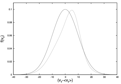
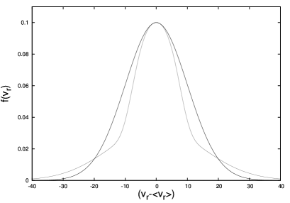
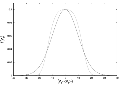
Figure 1: These four plots show one-dimensional velocity distribution functions for different cases. top: Gaussian velocity distribution describing thermodynamical equilibrium with a variance of $\sigma=10\,\text{km}/\text{s}$. The Gaussian appears in the subsequent panels for comparison (black). upper middle: velocity distribution (grey) with a skewness in positive $v_{r}$-direction indicating energy flow in $v_{r}$-direction. lower middle and bottom: two velocity distributions (grey) with an excess and deficit of high velocity stars respectively as compared to “thermodynamical equilibrium”

Neglecting third and fourth order moments in these cases results in a loss of information by failing to fully model the effect of the processes they represent on the evolution of the cluster.

2 Particle-based techniques vs statistical methods

The methods for studying star clusters can be divided into two types; statistical continuum models, such as Fokker-Planck (FP), or moment models and particle-based techniques, such as direct $N$-body models and Monte Carlo. They have different advantages and deliver complementary information about the processes and mechanisms that drive the evolution of star clusters.

2.1 Direct integration techniques

By using direct $N$-body we integrate Newton’s equations of motion. In principle all gravitational dynamics phenomena are naturally included in the integration. Thus, this method is not subject to any approximations nor restricted to any assumptions, such as spherical symmetry. In contrast to statistical methods, it does not require additional physics in order to include gravitational interactions between pairs, triples (binary-star interactions) or quadruples (binary-binary interactions) as they are inherent to the model. Including a mass spectrum or tidal field is also, in principle, straightforward. On the other hand, direct-summation methods of this type are computationally expensive, and as a consequence it is not possible to realistically model a stellar cluster with a typical number of $10^{7-8}$ stars. This is due to the fact that the computation of all pairwise interactions of a system consisting of $N$ particles scales with $N^{2-3}$. Using modern hardware we are severely limited to integrations of at most a few $10^{6}$ particles for a very short time, typically a few dynamical times. Another drawback of direct $N$-body is that it suffers from noise, as an individual N-body calculation in star cluster dynamics have exponential instabilities; nevertheless, the results can be used in a statistical average (e.g. Miller 1964; Giersz & Heggie 1994a).

There exist many schemes for integrating Newton’s gravitational equation, some of them are faster and more effective than others. Among these we should mention the Euler scheme or an improvement of this, the leapfrog scheme (e.g. Hut et al. 1995). We can gain more accuracy by the divided difference scheme or the Hermite scheme (Makino & Aarseth 1992; Aarseth 1999), which is used in the NBODY6 and NBODY6++ codes for the orbit integration. Additionally, various $N$-body codes incorporate a number of approaches which are necessary for maintaining adequate accuracy and efficiency over many dynamical times; these include the use of many individual time steps, computation of forces from near neighbors and distant stars with different frequencies, special treatments of compact pairs (binaries) and other few-body configurations (Mikkola & Aarseth 1990, 1993). Direct $N$-body simulation is a powerful tool for realistically simulating a wide range of astrophysically interesting scenarios such as black holes in galactic nuclei or GCs, binaries of massive black holes in (rotating) clusters (Amaro-Seoane & Freitag 2006; Amaro-Seoane et al. 2009, 2010) or binary black hole mergers in galactic nuclei (Berentzen et al. 2009).

2.2 The Monte Carlo approach

Other powerful particle-based techniques are the Monte Carlo (MC) methods, in which relaxation is treated using the Fokker-Planck approximation. These methods rely also on the assumptions that the system is spherically symmetric and that the gravitational potential can be separated into two parts. The advantage of MC is that it is orders of magnitude faster than direct $N-$body, yet it is still slower than statistical methods and also suffers from numerical noise.

Spitzer and collaborators pioneered the MC scheme in a series of papers, such as Spitzer & Hart (1971a, b); Spitzer & Shapiro (1972); Spitzer & Thuan (1972); Spitzer & Chevalier (1973); Spitzer & Shull (1975a, b); Spitzer & Mathieu (1980) The initial models were soon improved by Shapiro and his collaborators (Shapiro & Marchant 1978; Marchant & Shapiro 1979, 1980; Duncan & Shapiro 1982; Shapiro 1984). MC, being particle-based, follows the individual stellar orbits and allows us to model processes occurring on both relaxation and crossing time scales. Spitzer’s method was used to explore a variety of important phenomena, including mass segregation, anisotropy of the velocity distribution, tidal shocking, and the role of primordial binary stars, to mention a few.

The second MC approach was devised by Hénon (1971a, b, 1972, 1975) and later improved by Stodółkiewicz (1982, 1986). In contrast to the models of Spitzer, Hénon’s models assumed dynamical equilibrium; the distribution function must also depend only on isolated integrals of motion. It is worth mentioning that it was the first scheme to break through the impasse of core collapse (Hénon 1975). The algorithm was further improved by Stodółkiewicz (1985) by including processes such as the formation of binaries by two- and three-body encounters, mass loss from stellar evolution and tidal shocking.

Giersz (1998, 2001) in a series of papers modeled $\omega$Cen (Giersz & Heggie 2003), M4 (Heggie & Giersz 2008), M67 (Giersz et al. 2008) and NGC 6397 (Giersz & Heggie 2009) with MC techniques. In these papers several additional improvements were also included, as two-body relaxation, most kinds of three- and four-body interactions involving of primordial binaries and those formed dynamically, the Galactic tide and the internal evolution of both single and binary stars. MC techniques can be coupled with continuum models to describe the stochastic process of binary formation energy generation and movement (Spurzem & Giersz 1996; Giersz & Spurzem 2000, 2003). This has been successfully used to examine the gravitational radiation from binary black holes in star clusters (Downing et al. 2009).

Joshi et al. (2000, 2001); Fregeau et al. (2003); Fregeau & Rasio (2007) developed a MC technique based on a modified version of Hénon’s algorithm for solving the Fokker-Planck equation. Their scheme includes a mass spectrum, stellar evolution, and primordial binary interactions and the direct integration of binary scattering interactions. The Hénon-type MC approach has been used by M. Freitag, who developed another MC code with the special purpose of studying semi-Keplerian systems. Applying this code he extensively studied the structure of galactic nuclei containing a central MBH (Freitag 2000; Freitag & Benz 2002; Freitag et al. 2006).

2.3 A statistical model: The Fokker-Planck technique

Fokker-Planck (FP) models are based on the direct numerical solution of the orbit-averaged FP equation. Cohn (1979, 1980) pioneered a direct numerical finite-difference solution of the 1-dimensional FP equation (for a phase space distribution function: $f=f(E)$). Similar methods had been developed for a fixed potential by Ipser (1977) and by Cohn & Kulsrud (1978), and since then different FP codes have been written independently by Inagaki & Wiyanto (1984) and by Chernoff & Weinberg (1990). Whereas Cohn’s formulation assumes spherical symmetry, codes which can handle a rotating cluster have been devised by Goodman (1983a) and Einsel & Spurzem (1996). Takahashi (1995, 1996, 1997) has developed FP models for GCs, based on the numerical solution of the orbit averaged 2D FP equation (i.e. solving the FP equation for the distribution $f=f(E,J^{2})$) as a function of energy and angular momentum, and thus accounting for anisotropy.

Drukier et al. (1999) followed with results from another 2D FP code based on the original idea of Cohn (1979). There have been several comparative studies (Giersz & Heggie 1994a, b, 1997; Takahashi 1995; Giersz & Spurzem 1994; Spurzem & Takahashi 1995; Freitag et al. 2006; Khalisi et al. 2007) showing that for isolated, non-rotating star clusters the results of FP simulations are generally in good agreement with those of $N$-body simulations. However, when a tidal boundary is included, discrepancies between $N$-body and FP models occur.

Also, Einsel & Spurzem (1999) found that rotating GCs collapse faster than non-rotating ones with a 2D FP technique that had a distribution function depending on the $z$-component of the angular momentum, $f=f(E,J_{z})$. Kim et al. (2002) improved the approach by including an energy source due to formation and hardening of three-body binaries. These two studies only investigated single-mass models. Later, Kim et al. (2004) extended this method to multi-mass systems, finding interesting results concerning segregation of mass and angular velocity with heavy stars in the cluster. Fiestas et al. (2006) have modeled rotating globular clusters and Fiestas & Spurzem (2010) included a star accreting black hole with a loss cone. Comparative studies for rotating star clusters between FP and $N$-body methods have been done as well by Boily (2000); Boily & Spurzem (2000); Ardi et al. (2005); Ernst et al. (2007); Kim et al. (2008). They produced fairly similar results, though there were small discrepancies in the core-collapse time.

2.4 Advantages and disadvantages of statistical models as compared to direct-summation techniques

¿From the three different techniques, direct $N$-body models appear as the most realistic model. However, as mentioned before, it suffers from exponential instabilities; small deviations in the initial conditions result in exponential divergence of the phase space distribution of the particles of the system (Miller 1964; Giersz & Heggie 1994a). These instabilities make it difficult to compare a realistic model of GCs to observational data. Statistical models produce averaged physical quantities and are better suited for comparison with observations.

Also, as $N$-body models are not restricted by boundary conditions such as spherical symmetry, they can be applied to the widest range of stellar dynamical systems and study them under the most diverse scenarios. This relies on a microscopic description of dynamical processes and translates into a complexity that requires a massive computational effort. As a consequence we depend on the development of hardware to push the number of particles that we can integrate forward. On the other hand, statistical continuum models which are based on a comparatively small set of differential equations are computationally cheap.

These algorithms have also the important property that the contribution of various dynamical processes to the overall evolution of a star cluster can be isolated. This is so because the different mechanisms have to be included separately by additional terms in the model equations. Therefore, it is possible to identify each mechanism and its effect.

The downside of statistical moment models is that they are subject to a large number of approximations. Some of these approximations are inherent in the approach, such as the description of the phase space distribution function by a finite number of its velocity moments. Additional approximations consist of the limitation in the number of processes included such as two-body relaxation, star-binary deflections, binary-binary encounters or anisotropy. Such processes are natural in $N$-body models. The bottom line is that in order to build up a detailed understanding of stellar dynamical systems we need the different properties of particle-based and statistical models.

3 Self-gravitating, conducting gas spheres

In the previous section we have given an overview on the different numerical tools to address stellar dynamics including relaxation. Now that we have highlighted the advantages of statistical methods, we introduce an interesting alternative to FP . More than 35 years ago Hachisu et al. (1978) and Lynden-Bell & Eggleton (1980) proposed transport process in a self-gravitating, conducting gas sphere as a way to mimic two-body stellar relaxation. Later, Bettwieser (1983); Bettwieser & Sugimoto (1984); Bettwieser & Spurzem (1986); Heggie (1984) Heggie & N. Ramamani (1989) and Louis & Spurzem (1991) implemented anisotropy and Giersz & Spurzem (1994) and Spurzem & Takahashi (1995) added a multi-mass distribution and improved the detailed form of the conductivities to have better accuracy. The resulting model is often called the anisotropic gaseous model (AGM). This allows us to compare with $N-$body models to calibrate the approach. Amaro-Seoane et al. (2004) addressed the accretion of stars on to a massive black hole by adding collisional terms corresponding to loss-cone physics as well as tidal effects and Spurzem et al. (2005) investigated the evolution and dissolution of star clusters under the combined influence of internal relaxation and external tidal fields.

In this approach, we emulate spherically symmetric systems as a continuum; relaxation is treated as a diffusive process in phase space using the FP equation. We employ the local approximation to simplify the FP equation by neglecting the diffusion in position. The idea behind this is that an encounter takes place in a volume that is much smaller than the dimensions of the whole system. We model energy transfer by a local heat flux equation with an appropriately tailored conductivity.

The basis of the equations of the model is the FP equation which describes the time evolution of the probability density function. Using spherical polar coordinates, the Boltzmann equation takes the form:

$$\frac{\partial f}{\partial t}+v_{\rm{r}}\frac{\partial f}{\partial r}+\dot{v}_{\rm{r}}\frac{\partial f}{\partial v_{\rm{r}}}+\dot{v}_{\rm{\phi}}\frac{\partial f}{\partial v_{\rm{\phi}}}+\dot{v}_{\rm{\theta}}\frac{\partial f}{\partial v_{\rm{\theta}}}=\left(\frac{\delta f}{\delta t}\right)_{FP}$$ (2)

In the last equation the right-hand side denotes that collisions are given in terms of the FP approximation. Due to symmetry, we can define a tangential velocity $v_{t}^{2}=v_{\rm{\phi}}^{2}+v_{\rm{\theta}}^{2}$, so that we have two velocities $v_{t}$ and $v_{r}$ to describe the system. The “centralized” moments are defined by multiplying the velocity distribution $f$ with powers of $v_{t}$ and $(v_{r}-\bar{v}_{r})$ and integrating over velocity space.

The term “centralized” means that the moments are defined with respect to the mean velocity components $\bar{v}_{r}=\langle v_{r}\rangle=u$ and $\bar{v}_{t}=\langle v_{t}\rangle=0$, because we assume spherical symmetry. The order of a moment is defined by $n+m$ where $n$ and $m$ are the powers of velocities in the definition of moments, i.e. $\int(v_{r}-\bar{v}_{r})^{n}v_{t}^{m}\,f\,\,\mathrm{d}^{3}v$. The moments defined this way correspond to the density of stars, $\rho$, the bulk velocity, $u$, the radial and tangential pressures, $p_{r}$ and $p_{t}$, and the radial and tangential kinetic energy fluxes, $F_{r}$ and $F_{t}$. In order to obtain the set of differential moment equations, we multiply equation (2) with powers of $v_{t}$ and $(v_{r}-\bar{v}_{r})$ and integrate it in velocity space. After some recasting the integrals can be substituted by the moments. Up to second order the moment equations are the continuity equation, the Euler equation (force) and radial and tangential energy equations:

$$\begin{split}&\frac{\partial\rho}{\partial t}+\frac{1}{r^{2}}\frac{\partial}{\partial r}(r^{2}u\rho)=0\\ &\frac{\partial u}{\partial t}+u\,\frac{\partial u}{\partial r}+\frac{GM_{r}}{r^{2}}+\frac{1}{\rho}\frac{\partial p_{r}}{\partial r}+2\frac{p_{r}-p_{t}}{\rho r}=0\\ &\frac{\partial p_{r}}{\partial t}+\frac{1}{r^{2}}\frac{\partial}{\partial r}(r^{2}up_{r})+2p_{r}\,\frac{\partial u}{\partial r}+\frac{1}{r^{2}}\frac{\partial}{\partial r}(r^{2}F_{r})-\frac{2F_{t}}{r}\\ &=-\frac{3}{5}\frac{p_{r}-p_{t}}{\lambda_{A}t_{\mathrm{rx}}}+\left(\frac{\delta p_{r}}{\delta t}\right)_{\rm{bin}3}\\ &\frac{\partial p_{t}}{\partial t}+\frac{1}{r^{2}}\frac{\partial}{\partial r}(r^{2}up_{t})+\frac{2p_{r}u}{r}+\frac{1}{2r^{2}}\frac{\partial}{\partial r}(r^{2}F_{t})+\frac{F_{t}}{r}=\\ &\frac{3}{10}\frac{p_{r}-p_{t}}{\lambda_{A}t_{\mathrm{rx}}}+\left(\frac{\delta p_{t}}{\delta t}\right)_{\rm{bin}3}\end{split}$$ (3)

Here $\lambda_{A}$ is a numerical constant related to the time-scale of collisional anisotropy decay, necessary to describe the relaxation effects on cluster evolution. It should become unity when describing GCs using higher moment models. However, this can only be confirmed by simulations. The value of $\lambda_{A}$ is discussed in Giersz & Spurzem (1994) and is chosen by calibrating with $N-$body simulations. The authors found that $\lambda_{A}=0.1$ is a physically realistic value within the half-mass radius for all numbers of particles.

The two terms on the right-hand sides of the equations for radial and tangential energy equations are the collisional terms. The fist term accounts for relaxation from uncorrelated two-body encounters and can be derived from the FP equation. The second term, which is marked with “bin3”, refers to star-binary encounters. Close 3-body or star-binary encounters generate kinetic energy. If the energy generation is high enough, this mechanism can reverse core collapse.

The radial and tangential pressure, $p_{r}$ and $p_{t}$ are related to the random velocity dispersions; $p_{r}=\rho\,\sigma_{r}^{2}$ and $p_{t}=\rho\,\sigma_{t}^{2}$. They are linked to observable quantities in stellar clusters such as the radial velocity dispersion. The average velocity dispersion is $\sigma^{2}=(\sigma_{r}^{2}+2\sigma_{t}^{2})/3$, where the factor 2 comes from the fact that there are two tangential directions. The radial energy flux of random kinetic energy is $F=(F_{r}+F_{t})/2$. We can see this by adding the two-moment equations for radial and tangential pressure to obtain the gas-dynamical equation for the energy density. The velocities for energy transport are defined by

$$\begin{split}&v_{r}=\frac{F_{r}}{3p_{r}}+u\\ &v_{t}=\frac{F_{t}}{2p_{t}}+u\end{split}$$ (4)

In the case of weak isotropy, $p_{r}=p_{t}$ everywhere and hence $F_{r}=\frac{3}{2}F_{t}$, so that $v_{r}=v_{t}$. Therefore, the transport velocities for radial and tangential random kinetic energy are equal.

In order to close the set of moment equations (LABEL:moment_equations) three more equations are set up, a mass relation and two equations accounting for heat flux. The mass relation defines the mass $M_{r}$ contained in a sphere of radius $r$,

$$\frac{\partial M_{r}}{\partial r}=4\pi r^{2}\rho_{M}$$ (5)

where $\rho_{M}=M\cdot\rho$ is the mass density and $M$ the mass of the stellar component. We thus obtain a set of gas dynamical equations (LABEL:moment_equations) coupled with the Poisson equation (25). Since the moment equations of order $n$ obtained from the Boltzmann equation contain moments of the order $n+1$, we need closure relations connecting the moments of order $n+1$ with lower-order moments. This is achieved with the heat conduction closure, a phenomenological approach obtained in an analogous way to gas dynamics. It is motivated by the resemblance between a star consisting of a large number of atoms and a star cluster with large number of stars not only on the simple level of the virial theorem but also due to similarities in heat transport, energy generation and core-halo evolution. It was used by Lynden-Bell & Eggleton (1980), initially restricted to isotropic systems. In this approximation we assume that heat transport is proportional to the temperature gradient

$$F=-\kappa\frac{\partial T}{\partial r}=-\Lambda\frac{\partial\sigma^{2}}{\partial r}$$ (6)

This equation describes the heat flux in gases and liquids and for this reason the models using this closure are also called conducting gas sphere models. Even though the use of equation (6) is based on the assumption of small mean free paths for the particles, which is certainly questionable for stellar dynamical systems, models like the AGM agree with other modeling methods (e.g. $N$-Body, FP) (Giersz & Spurzem 1994; Spurzem & Takahashi 1995)

In the classical approach $\Lambda\propto\rho\bar{\lambda}^{2}/\tau$, where $\bar{\lambda}$ is the mean free path and $\tau$ the collisional time. Choosing the Jeans length $\lambda_{J}^{2}=\sigma^{2}/(4\pi G\rho)$ for $\bar{\lambda}^{2}$ and the standard Chandrasekhar local relaxation time $t_{\rm{rx}}\propto\sigma^{3}/\rho$ (Chandrasekhar 1942) for $\tau$, we obtain the conductivity $\Lambda\propto\rho/\sigma$. More precisely, the conductivity takes the form found in Lynden-Bell & Eggleton (1980):

$$\Lambda=\frac{3CGm\rho N}{\sigma},$$ (7)

where C is a dimensionless numerical constant of order unity. By means of the velocities of energy transport the heat flux equation can be recast to find the two closure relations in the anisotropic case

$$v_{r}-u+\frac{\lambda}{4\pi G\rho t_{\rm{rx}}}\frac{\partial\sigma^{2}}{\partial r}=0\qquad v_{r}=v_{t},$$ (8)

where

$$\lambda=\frac{27\sqrt{\pi}}{10}C$$ (9)

It should be emphasized that $\lambda$ is a free parameter that has to be determined by comparison with other models such as $N$-body (Giersz & Spurzem 1994), Louis’ fluid dynamical model (Louis & Spurzem 1991) or FP models. In the isotropic limit, $\lambda$ is just a scaling scaling factor, but when taking into account anisotropy, $\lambda$ prescribes the relative speed of two processes: the decay of anisotropy and the heat flow between warm and cold regions. With increasing $\lambda$ heat flows faster, so there is less time for gravitational encounters to destroy anisotropy. A larger $\lambda$ thus results in stronger anisotropy.

4 Higher moment models

In this section we present a new higher order moment model. We derive the model equations which consist of differential equations for the velocity moments of the phase space distribution function, a Poisson equation and three equations to close the system of equations. We first compute the left-hand sides of the differential moment equation and then use a polynomial ansatz for the phase space distribution function to obtain the right-hand sides. We define two models, model a and model b, which differ in the number of differential (moment) equations and their closure relation.

4.1 Left-hand sides

Without collisions, the Boltzmann equation takes the form of a conservation equation ($\mathrm{d}f/\mathrm{d}t=0$) and describes the advective rate of change of the phase space distribution function $f$. If we follow the trajectory of a particle in a system described by the collisionless Boltzmann equation, the number density in phase space around the particle does not change. This implies that flow in phase space is incompressible. It becomes compressible when collisions are introduced with FP terms on the right hand side of the Boltzmann equation.

Assuming that the stellar system is spherically symmetric, we can use spherical coordinates when we write the collisional Boltzmann equation,

$$\frac{\partial f}{\partial t}+v_{r}\frac{\partial f}{\partial r}+\dot{v}_{r}\frac{\partial f}{\partial v_{r}}+\dot{v}_{\theta}\frac{\partial f}{\partial v_{\theta}}+\dot{v}_{\phi}\frac{\partial f}{\partial v_{\phi}}=\left(\frac{\delta f}{\delta t}\right)_{\text{enc}}$$ (10)

Using the Lagrangian of a particle in a spherical symmetric potential $\Phi(r,t)$, we have that

$$\mathcal{L}=\frac{1}{2}(\dot{r}^{2}+r^{2}\dot{\theta}^{2}+r^{2}\sin^{2}\theta\,\dot{\phi}^{2})-\Phi(r,t)$$ (11)

We then apply the Euler-Lagrange equations to the Lagrangian, to derive the equations of motion

$$\dot{v}_{r} = -\frac{\partial\Phi}{\partial r}+\frac{v^{2}_{\theta}+v^{2}_{\phi}}{r}$$

$$\dot{v}_{\theta} = -\frac{v_{r}v_{\theta}}{r}+\frac{v^{2}_{\phi}}{r\tan\theta}$$ (12)

$$\dot{v}_{\phi} = -\frac{v_{r}v_{\phi}}{r}-\frac{v_{\theta}v_{\phi}}{r\tan\theta}$$

After substituting equation (4.1) into the Boltzmann equation (10), we use the approach of spherical symmetry to define the tangential velocity $v_{t}=\sqrt{v^{2}_{\theta}+v^{2}_{\phi}}$ and obtain

$$\frac{\partial f}{\partial t}+v_{r}\frac{\partial f}{\partial r}+\left(\frac{v^{2}_{t}}{r}-\frac{\partial\Phi}{\partial r}\right)\frac{\partial f}{\partial v_{r}}-\frac{v_{r}v_{t}}{r}\frac{\partial f}{\partial v_{t}}=\left(\frac{\delta f}{\delta t}\right)_{\text{enc}}$$ (13)

We now define the velocity moments of the distribution function $f=f(r,v_{r},v_{t},t)$ by multiplying it by powers of $v_{r}$ and $v_{t}$ and integrating over velocity space,

$$[n,m]=\int\textnormal{d}^{3}v\,f\,v^{n}_{r}\,v^{m}_{t}=2\pi\int^{\infty}_{0}\textnormal{d}v_{t}\int^{\infty}_{-\infty}\textnormal{d}v_{r}\,f\,v^{n}_{r}\,v^{m+1}_{t}$$ (14)

Again, the order of a moment is defined as $k=n+m$. To obtain the differential equations for the moments $[n,m]$ we multiply equation (13) with powers of $v_{r}$ and $v_{t}$ and integrate over velocity space. After some recasting we can substitute the integrals by $[n,m]$ which yields

$$\begin{split}&\frac{\partial}{\partial t}[n,m]+\frac{\partial}{\partial r}[n+1,m]+\frac{m+2}{r}[n+1,m]\\ &-\frac{n}{r}[n-1,m+2]+n[n-1,m]\frac{\partial\Phi}{\partial r}=\left(\frac{\delta}{\delta t}[n,m]\right)_{\text{enc}}\end{split}$$ (15)

We now want to find a differential equation equivalent to equation (LABEL:eq:moment_dgl) for centralized moments. The centralized velocity moments are defined with respect to their mean velocity. Due to the assumed spherical symmetry of the system the mean velocities of the tangential components $\bar{v}_{\theta}=\bar{v}_{\phi}=0$ vanish. The mean velocity is only given by the radial velocity component

$$\bar{v}_{r}=[1,0]=u=2\pi\int^{\infty}_{0}\textnormal{d}v_{t}\int^{\infty}_{-\infty}\textnormal{d}v_{r}\,f\,v_{r}\,v_{t}$$ (16)

We hence obtain the definition for centralized moments by substituting $v_{r}$ in equation (14) with $(v_{r}-\bar{v}_{r})$. Furthermore, the centralized moments can be expressed in terms of the moments $[n,m]$ and are defined as

$$\langle n,m\rangle = \int\textnormal{d}^{3}v\,(v_{r}-\bar{v}_{r})^{n}\,v^{m}_{t}\,f$$

$$= 2\pi\int^{\infty}_{0}\textnormal{d}v_{t}\int^{\infty}_{-\infty}\textnormal{d}v_{r}\,(v_{r}-\bar{v}_{r})^{n}\,v^{m+1}_{t}\,f$$

$$= \sum^{n}_{k=0}\binom{n}{k}\,(-1)^{n-k}\,[1,0]^{n-k}\,[k,m]$$

It is evident from the second line of (4.1) that the first centralized moment $\langle 1,0\rangle=0$.

We adopt the following notation for the centralized moments:

$$\begin{split}\rho&=\langle 0,0\rangle\qquad\langle 1,0\rangle=0\\ p_{r}&=\langle 2,0\rangle\qquad 2p_{t}=\langle 0,2\rangle\\ F_{r}&=\langle 3,0\rangle\qquad F_{t}=\langle 1,2\rangle\\ \kappa_{r}&=\langle 4,0\rangle\qquad\kappa_{rt}=\langle 2,2\rangle\qquad\kappa_{t}=\langle 0,4\rangle\\ G_{r}&=\langle 5,0\rangle\qquad G_{rt}=\langle 3,2\rangle\qquad G_{t}=\langle 1,4\rangle\\ H_{r}&=\langle 6,0\rangle\qquad H_{r,t}=\langle 4,2\rangle\qquad H_{t,r}=\langle 2,4\rangle\qquad H_{t}=\langle 0,6\rangle\end{split}$$ (18)

Again, $\rho$ is the particle density, $p_{r}$ and $p_{t}$ are the radial and tangential pressure and are related to the radial and tangential velocity dispersion $\sigma_{r}=p_{r}/\rho$ and $\sigma_{t}=p_{t}/\rho$, and $F_{r}$ and $F_{t}$ denote the radial and tangential energy flux.

We obtain a linear system of equations which can be solved for the moments $[n,m]$ by computing all centralized moments $\langle n,m\rangle$ up to order $n+m=6$ using equation (4.1):

$$\begin{split}&[2,0]=p_{r}+\rho u^{2}\\ &[0,2]=2p_{t}\\ &[3,0]=\rho u^{3}+3up_{r}+F_{r}\\ &[1,2]=2up_{t}+F_{t}\\ &[4,0]=\rho u^{4}+6u^{2}p_{r}+4uF_{r}+\kappa_{r}\\ &[2,2]=2u^{2}p_{t}+2uF_{t}+\kappa_{rt}\\ &[0,4]=\kappa_{t}\\ &[5,0]=\rho u^{5}+10u^{3}p_{r}+10u^{2}F_{r}+5u\kappa_{r}+G_{r}\\ &[3,2]=2u^{3}p_{t}+3u^{2}F_{t}+3u\kappa_{rt}+G_{rt}\\ &[1,4]=u\kappa_{t}+G_{t}\\ &[6,0]=\rho u^{6}+15u^{4}p_{r}+20u^{3}F_{r}+15u^{2}\kappa_{r}+6uG_{r}+H_{r}\\ &[4,2]=2u^{4}p_{t}+4u^{3}F_{t}+6u^{2}\kappa_{rt}+4uG_{rt}+H_{rt}\\ &[2,4]=u^{2}\kappa_{t}+2uG_{t}+H_{tr}\\ &[0,6]=H_{t}\end{split}$$ (19)

To obtain the differential equations for the centralized moments, we substitute the transformation from equation (LABEL:eq:transform) into equation (LABEL:eq:moment_dgl) and then successively use differential equations for lower-order moments to simplify the differential equations for higher orders. We divide the differential moment equations into three sets, defined as follows

Set I :

$$\begin{split}&\frac{\partial\rho}{\partial t}+\textnormal{div}(\rho u)=\left(\frac{\delta\rho}{\delta t}\right)_{\text{enc}}\\ &\frac{\partial\rho u}{\partial t}+\textnormal{div}(\rho u^{2})+\frac{\partial p_{r}}{\partial r}+\frac{2}{r}(p_{r}-p_{t})+\rho\frac{\partial\Phi}{\partial r}=\left(\frac{\delta\rho u}{\delta t}\right)_{\text{enc}}\\ &\frac{\partial p_{r}}{\partial t}+\textnormal{div}(F_{r}+up_{r})+2p_{r}\frac{\partial u}{\partial r}-\frac{2}{r}F_{t}=\left(\frac{\delta p_{r}}{\delta t}\right)_{\text{enc}}\\ &2\frac{\partial p_{t}}{\partial t}+\textnormal{div}(F_{t}+2up_{t})+\frac{2}{r}(F_{t}+2up_{t})=2\left(\frac{\delta p_{t}}{\delta t}\right)_{\text{enc}}\\ \end{split}$$ (20)

Set II :

$$\begin{split}&\frac{\partial F_{r}}{\partial t}+\textnormal{div}(\kappa_{r}+uF_{r})+3F_{r}\frac{\partial u}{\partial r}\\ &-3\frac{p_{r}}{\rho}\textnormal{div}p_{r}-\frac{3}{r}(\kappa_{rt}-\frac{2p_{r}p_{t}}{\rho})=\left(\frac{\delta F_{r}}{\delta t}\right)_{\text{enc}}\\ &\frac{\partial F_{t}}{\partial t}+\textnormal{div}(\kappa_{rt}+uF_{t})+F_{t}\frac{\partial u}{\partial r}-\frac{2p_{t}}{\rho}\textnormal{div}p_{r}\\ &-\frac{1}{r}(\kappa_{t}-2\kappa_{rt}-2uF_{t}-4\frac{p_{t}^{2}}{\rho})=\left(\frac{\delta F_{t}}{\delta t}\right)_{\text{enc}}\\ &\frac{\partial\kappa_{r}}{\partial t}+\textnormal{div}(G_{r}+u\kappa_{r})+4\kappa_{r}\frac{\partial u}{\partial r}-4\frac{F_{r}}{\rho}\textnormal{div}p_{r}\\ &-\frac{4}{r}(G_{rt}-\frac{2p_{t}F_{r}}{\rho})=\left(\frac{\delta\kappa_{r}}{\delta t}\right)_{\text{enc}}\\ &\frac{\partial\kappa_{rt}}{\partial t}+\textnormal{div}(G_{rt}+u\kappa_{rt})+2\kappa_{rt}\frac{\partial u}{\partial r}-2\frac{F_{t}}{\rho}\textnormal{div}p_{r}\\ &+\frac{2}{r}(G_{rt}-G_{t}+u\kappa_{rt}+2\frac{p_{t}F_{t}}{\rho})=\left(\frac{\delta\kappa_{rt}}{\delta t}\right)_{\text{enc}}\\ &\frac{\partial\kappa_{t}}{\partial t}+\textnormal{div}(G_{t}+u\kappa_{t})+\frac{4}{r}(G_{t}+u\kappa_{t})=\left(\frac{\delta\kappa_{t}}{\delta t}\right)_{\text{enc}}\\ \end{split}$$ (21)

Set III :

$$\begin{split}&\frac{\partial G_{r}}{\partial t}+\text{div}(H_{r}+uG_{r})+5G_{r}\frac{\partial u}{\partial r}-5\frac{\kappa_{r}}{\rho}\text{div}p_{r}\\ &-\frac{5}{r}(H_{rt}-2\frac{p_{t}\kappa_{r}}{\rho})=\left(\frac{\delta G_{r}}{\delta t}\right)_{\text{enc}}\\ &\frac{\partial G_{rt}}{\partial t}+\text{div}(H_{rt}+uG_{rt})+3G_{rt}\frac{\partial u}{\partial r}-3\frac{\kappa_{rt}}{\rho}\text{div}p_{r}\\ &+\frac{1}{r}(2H_{rt}-3H_{tr}+2uG_{rt}+6\frac{p_{t}\kappa_{rt}}{\rho})=\left(\frac{\delta G_{rt}}{\delta t}\right)_{\text{enc}}\\ &\frac{\partial G_{t}}{\partial t}+\text{div}(H_{tr}+uG_{t})+G_{t}\frac{\partial u}{\partial r}-\frac{\kappa_{t}}{\rho}\text{div}p_{r}\\ &-\frac{1}{r}(H_{t}-4H_{tr}-4uG_{t}-2\frac{p_{t}\kappa_{t}}{\rho})=\left(\frac{\delta G_{t}}{\delta t}\right)_{\text{enc}}\\ \end{split}$$ (22)

Note that the divergence operator in spherical symmetry reduces to:

$$\text{div}=\frac{1}{r^{2}}\frac{\partial}{\partial r}\,r^{2}$$ (23)

We now define two models with different accuracies,

Model a

– including (LABEL:moment_equations_a) and (LABEL:moment_equations_b)

Model b

– including all, (LABEL:moment_equations_a), (LABEL:moment_equations_b) and (LABEL:moment_equations_c)

The potential $\Phi(r,t)$ is determined by the fraction of cluster mass $M_{r}(t)$ contained at radius $r$

$$\Phi=-\frac{GM_{r}}{r}$$ (24)

$\Phi$ obeys the Poisson equation $\Delta\Phi=4\pi\rho_{\text{M}}$, where $\rho_{\text{M}}=M\rho$ is the mass density of the cluster. This leads to the equation for $M_{r}$

$$\frac{\partial M_{r}}{\partial r}=4\pi r^{2}\rho_{\text{M}}$$ (25)

We note that the moment equations of order $n$ contain moments of order $n+1$. To close the system of equations we need closure equation where moments of order $n+1$ are expressed with lower-order moments. We derive these relations in the next section.

4.2 FP collision terms

We now compute the right-hand sides of the differential moment equations (LABEL:moment_equations_a), (LABEL:moment_equations_b) and (LABEL:moment_equations_c), i.e. the collisional terms. Our starting point is the collisional Boltzmann equation (10). We have to find an expression for the term $(\delta f/\delta t)_{\text{enc}}$. This can be done by approximating it with the Fokker-Planck equation, which requires that the evolution of the stellar system is driven by uncorrelated distant encounters.

The Fokker-Planck equation is a diffusion equation that describes the diffusion of the phase space distribution function in position and velocity space. We assume that the volume in which a stellar encounter takes place is small when compared to the volume of the whole system. As a consequence, we can assume that during an encounter only the velocity of the particle is modified, but not the position. We thus neglect the diffusion of the phase space distribution function in position space. This approach is usually referred to as the “local approximation”. Therefore, the right-hand side of equation (10) is

$$\begin{split}\left(\frac{\delta f}{\delta t}\right)_{\text{enc}}=&-\sum^{3}_{i=1}\left[\frac{\partial}{\partial v_{i}}\left(f(\vec{x},\vec{v})D(\Delta v_{i})\right)\right]\\ &+\frac{1}{2}\sum^{3}_{i,j=1}\bigg{[}\frac{\partial^{2}}{\partial v_{i}\partial v_{j}}\left(f(\vec{x},\vec{v})D(\Delta v_{i}\Delta v_{j})\right)\bigg{]}\end{split}$$ (26)

$D(\Delta v_{i})$ and $D(\Delta v_{i}\Delta v_{j})$ are the diffusion coefficients which depend on position and velocity coordinates. They determine the diffusion of the phase space distribution function in velocity space and describe the average change of the $i$-th component of velocity per unit time due to stellar collisions. This is expressed by their dependence on the change of the $i$th velocity component $\Delta v_{i}$. Note that there are no diffusion coefficients that depend on $\Delta x_{i}$ as we are using the local approximation. The diffusion coefficients are (Rosenbluth et al. 1957):

$$\begin{split}D(\Delta v_{i})&=4\pi G^{2}m_{f}\ln\Lambda\frac{\partial}{\partial v_{i}}h(\vec{v})\\ D(\Delta v_{i}\Delta v_{i})&=4\pi G^{2}m_{f}\ln\Lambda\frac{\partial^{2}}{\partial v_{i}\partial v_{j}}g(\vec{v})\end{split}$$ (27)

$\ln\Lambda$ is the Coulomb logarithm, where $\Lambda$ is the ratio between the upper and lower cut-off impact parameter $b$ in a stellar collision. $h(\vec{v})$ and $g(\vec{v})$ are called the Rosenbluth potentials which are given by

$$\begin{split}h(\vec{v})&=(m+m_{f})\int\frac{f(\vec{v_{f}})}{|\vec{v}-\vec{v}_{f}|}\text{d}^{3}\vec{v}_{f}\\ g(\vec{v})&=m_{f}\int f(\vec{v_{f}})|\vec{v}-\vec{v}_{f}|\text{d}^{3}\vec{v}_{f}\end{split}$$ (28)

Thus, $m$ denotes the mass of a test star that moves through a distribution $f(V_{f},\mu_{f})$ of field stars with a mass $m_{f}$. The FP equation then takes the form:

$$\begin{split}\left(\frac{\delta f}{\delta t}\right)_{\text{enc}}=&-4\pi G^{2}m_{f}\ln\Lambda\bigg{[}\sum^{3}_{i=1}\frac{\partial}{\partial v_{i}}\left(f(\vec{v})\frac{\partial h}{\partial v_{i}}\right)\\ &-\frac{1}{2}\sum^{3}_{i,j=1}\frac{\partial^{2}}{\partial v_{i}\partial v_{j}}\left(f(\vec{v})\frac{\partial^{2}g}{\partial v_{i}\partial v_{j}}\right)\bigg{]}\end{split}$$ (29)

To compute this expression we need to know the phase space distribution function $f(\vec{r},\vec{v},t)$. We approximate the distribution function by a series expansion which accounts for the spherical symmetry of the system (see e.g. Rosenbluth et al. 1957; Larson 1970). The expansion coefficients are expressed in terms of the velocity moments needed to compute the collisional terms of the moment equations. We then compute the phase space distribution function $f$ to calculate the Rosenbluth potentials $h$ and $g$, the right-hand side of the FP equation and thus the collisional terms of the Boltzmann equation.

4.2.1 Construction of the distribution function

The phase space distribution function in spherical symmetry only depends on $r$, $v_{r}$, $v^{2}_{\theta}+v^{2}_{\phi}$, and $t$, i.e. $f=f(r,v_{r},v^{2}_{\theta}+v^{2}_{\phi},t)$, which implies that the system is axially symmetric in the velocity space with axes $v_{r}$, $v_{\theta}$ and $v_{\phi}$. The velocity components can be written in spherical coordinates

$$v_{r}-\bar{v}_{r} = V\,\cos\theta^{\prime}$$

$$v_{\theta} = V\,\sin\theta^{\prime}\,\cos\phi^{\prime}$$ (30)

$$v_{\phi} = V\,\sin\theta^{\prime}\,\sin\phi^{\prime},$$

where $V$ is the modulus of $\vec{v}$ , $\theta^{\prime}$ the angle between $\vec{v}$ and the radial direction, and $\phi^{\prime}$ the angle which defines the orientation of the tangential component of $\vec{v}$ in the $v_{\theta}v_{\phi}$-plane. Note that our model describes non-rotational spherically symmetric systems and thus the mean tangential velocities are $\bar{v}_{\theta}=\bar{v}_{\phi}=0$. Thus, equations (4.2.1) denote the components of the radial and tangential velocities with respect to their means. As the phase space distribution function $f$ only depends on $v^{2}_{\theta}+v^{2}_{\phi}$, it is independent on the angle $\phi^{\prime}$. We can henceforth omit the prime from angle $\theta^{\prime}$.

Since we are operating in velocity space, in the following we refer to $f$ as the (local) velocity distribution function (VDF). Substituting $\mu=\cos\theta$ yields

$$v_{r}-\bar{v}_{r}=V\mu,\qquad v^{2}_{t}=v^{2}_{\theta}+v^{2}_{\phi}=V^{2}(1-\mu^{2})$$ (31)

These coordinates are appropriate for a series expansion of the VDF in Legendre polynomials (Larson 1970):

$$\begin{split}f(V,\mu)&=g(V)+\sum_{l=0}^{\infty}a_{l}(V)P_{l}(\mu)\\ &=\sum^{\infty}_{l=0}A_{l}(V)P_{l}(\mu)\end{split}$$ (32)

where $A_{0}(V)=g(V)+a_{0}(V)$ and $A_{l}(V)=a_{l}(V)$ for $l\geq 1$. In this expansion

$$g(V)=\rho\frac{1}{\sqrt{2\pi}\sigma^{3}}\exp(-\frac{V^{2}}{\sigma^{2}})$$

Thus $g(V)V^{2}$ is the Maxwell-Boltzmann (MB) VDF. $P_{l}(\mu)$ are the Legendre polynomials, and the functions $a_{i}(V)$ are defined by

$$a_{i}(V)=g(V)\sum_{j=0}^{l_{max}}c_{ij}V^{j}$$

where $l_{max}$ denotes the highest order of the Legendre polynomials $P_{l}(\mu)$ in the expansion of the VDF. Due to axial symmetry in velocity space the VDF can only depend on powers of $v_{t}$ and $v_{r}$. Using equations (31) and fully expanding the VDF we find the following constraints for the coefficients $c_{nm}$:

• $n\leq m$

• $n$ and $m$ are either both even or both odd

otherwise $c_{ij}=0$.

We obtain for model b a VDF which extends to order $l=5$ in the Legendre Polynomials $P_{l}(\mu)$ which reads

$$\begin{split}f(V,\mu)=&\,g(V)+g(V)(c_{00}+c_{02}V^{2}+c_{04}V^{4})P_{0}(\mu)\\ &+g(V)(c_{11}V+c_{13}V^{3}+c_{15}V^{5})P_{1}(\mu)\\ &+g(V)(c_{22}V^{2}+c_{24}V^{4})P_{2}(\mu)\\ &+g(V)(c_{33}V^{3}+c_{35}V^{5})P_{3}(\mu)+g(V)c_{44}V^{4}P_{4}(V)\\ &+g(V)V^{5}c_{55}P_{5}(\mu)\end{split}$$ (33)

The VDF for model a only extends to order $l=4$ and can be obtained from equation (33) by setting all coefficients $c_{ij}$ with $j>4$ to zero.

We can now calculate the coefficients $c_{ij}$ using the definition of the centralized moments from equation (4.1). However, we first have to transform equation (4.1) to the new coordinate system $(V,\mu)$. The volume element $\text{d}^{3}v$ in these coordinates is written as:

$$\textnormal{d}^{3}v=V^{2}\,\rm{d}V\,\rm{d}(\cos\theta)\,\rm{d}\phi=V^{2}\,\rm{d}V\,\rm{d}\mu\,\rm{d}\phi\quad\textnormal{where}\quad\mu=\cos\theta$$ (34)

Thus we obtain for the centralized moments:

$$\langle n,m\rangle = \int\textnormal{d}^{3}vf\,(v_{r}-u)^{n}v_{t}^{m}$$ (35)

$$= \int V^{2}\textnormal{d}V\,\textnormal{d}\mu\,\textnormal{d}\phi\,f\,(v_{r}-u)^{n}v_{t}^{m}$$

$$= 2\pi\int V^{2}\textnormal{d}V\textnormal{d}\mu\,f\,V^{n}\mu^{n}(V^{2}(1-\mu^{2}))^{m/2}$$

$$= 2\pi\int\textnormal{d}V\,\textnormal{d}\mu\,f\,V^{2+n+m}\mu^{n}(1-\mu^{2})^{m/2}$$

We can obtain a linear system of equations to be solved for the coefficients $c_{ij}$ by computing the different moments via this equation with the expansion of the VDF from equation (33). It must be noted that:

• The first centralized moment vanishes, since $\langle v_{r}-\bar{v}_{r}\rangle=\bar{v}_{r}-\bar{v}_{r}=0$, i.e.

  $$\langle 1,0\rangle=0$$ (36)

• Since there are two tangential directions we add a factor 2 in the definition below

  $$2p_{t}=\langle 0,2\rangle$$ (37)

We obtain for the VDF of model a the coefficients $c_{ij}$:

$$\begin{split}&c_{00}=\frac{27}{8}-\frac{7(p_{r}+2p_{t})}{4\rho\sigma^{2}}+\frac{\kappa_{r}+2\kappa_{rt}+\kappa_{t}}{8\rho\sigma^{4}}\\ &c_{02}=-\frac{7}{4\sigma^{2}}+\frac{p_{r}+2p_{t}}{\rho\sigma^{4}}-\frac{\kappa_{r}+2\kappa_{rt}+\kappa_{t}}{12\rho\sigma^{6}}\\ &c_{04}=\frac{1}{8\sigma^{4}}-\frac{p_{r}+2p_{t}}{12\rho\sigma^{6}}+\frac{\kappa_{r}+2\kappa_{rt}+\kappa_{t}}{120\rho\sigma^{8}}\\ &c_{11}=-\frac{F_{r}+F_{t}}{2\rho\sigma^{4}}\\ &c_{13}=\frac{F_{r}+F_{t}}{10\rho\sigma^{6}}\\ &c_{22}=\frac{3(p_{r}-p_{t})}{2\rho\sigma^{4}}-\frac{2\kappa_{r}+\kappa_{\text{rt}}-\kappa_{t}}{12\rho\sigma^{6}}\\ &c_{24}=-\frac{p_{r}-p_{t}}{6\rho\sigma^{6}}+\frac{2\kappa_{r}+\kappa_{\text{rt}}-\kappa_{t}}{84\rho\sigma^{8}}\\ &c_{33}=\frac{F_{r}-\frac{3}{2}F_{t}}{15\rho\sigma^{6}}\\ &c_{44}=\frac{\frac{1}{3}\kappa_{r}-\kappa_{\text{rt}}+\frac{1}{8}\kappa_{t}}{35\rho\sigma^{8}}\end{split}$$ (38)

Since the coefficients $c_{ij}$ with $i=0,1$ only depend on sums of moments, we can find a definition for total moments (see section 5.1).

The role of anisotropy comes into the open when going to higher-order coefficients, like $c_{2j}\propto(p_{r}-p_{t})\propto a$, where $a=1-{p_{t}}/{p_{r}}$ is the anisotropy parameter. We envisage a system as isotropic in a “weak” sense if $a=0$ everywhere. Strong isotropy holds if the distribution has the strict dependence $f=f(r,(v_{r}-\bar{v}_{r})^{2}+(v^{2}_{\theta}+v^{2}_{\phi})^{2},t)=f(r,V,t)$ on the modulus of the velocity, which results in $F_{r}=F_{t}=0$ for the radial and tangential energy flux, i.e. spherical symmetry in velocity space. We now compute the moments of fifth order with the VDF of model a. In this case the expansion in Legendre polynomials $P_{l}(\mu)$ expands up to $l=4$ and the fifth order moments are

$$G_{r}=10\sigma^{2}F_{r},\qquad G_{rt}=2\sigma^{2}F_{r}+3\sigma^{2}F_{t},\qquad G_{t}=8\sigma^{2}F_{t}$$ (39)

As we saw before, the system of differential moment equations (LABEL:moment_equations_a) and (LABEL:moment_equations_b) combined with the mass relation (25) was not complete. We can now close it by including the three relations in equation (39). In these equations the fifth-order moments $G$ are expressed through lower-order moments. We now have a set of equations ((LABEL:moment_equations_a), (LABEL:moment_equations_b), (25) and (39)) that is numerically solvable. This set describes our model a.

Combining the three relations we have

$$G_{r}-5G_{rt}+\frac{15}{8}G_{t}=0$$ (40)

We will see that the left-hand side of equation (40) appears in the coefficient $c_{55}$ when the coefficients $c_{ij}$ of the VDF of model b are computed. It then becomes clear that equation (40) is a result of setting $c_{55}=0$ since $c_{44}$ is the highest coefficient of the VDF of model a.

For the VDF of model b we find

$$\begin{split}c_{00}=&\frac{27}{8}-\frac{7(p_{r}+2p_{t})}{4\rho\sigma^{2}}+\frac{(\kappa_{r}+2\kappa_{rt}+\kappa_{t})}{8\rho\sigma^{4}}\\ c_{02}=&-\frac{7}{4\sigma^{2}}+\frac{(p_{r}+2p_{t})}{\rho\sigma^{4}}-\frac{(\kappa_{r}+2\kappa_{rt}+\kappa_{t})}{12\rho\sigma^{6}}\\ c_{04}=&\frac{1}{8\sigma^{4}}-\frac{(p_{r}+2p_{t})}{12\rho\sigma^{6}}+\frac{(\kappa_{r}+2\kappa_{rt}+\kappa_{t})}{120\rho\sigma^{8}}\\ c_{11}=&-\frac{9(F_{r}+F_{t})}{4\rho\sigma^{4}}+\frac{G_{r}+2G_{rt}+G_{t}}{8\rho\sigma^{6}}\\ c_{13}=&\frac{4(F_{r}+F_{t})}{5\rho\sigma^{6}}-\frac{G_{r}+2G_{rt}+G_{t}}{20\rho\sigma^{8}}\\ c_{15}=&-\frac{F_{r}+F_{t}}{20\rho\sigma^{8}}+\frac{G_{r}+2G_{rt}+G_{t}}{280\rho\sigma^{10}}\\ c_{22}=&\frac{3(p_{r}-p_{t})}{2\rho\sigma^{4}}-\frac{(2\kappa_{r}+\kappa_{\text{rt}}-\kappa_{t})}{12\rho\sigma^{6}}\\ c_{24}=&-\frac{(p_{r}-p_{t})}{6\rho\sigma^{6}}+\frac{(2\kappa_{r}+\kappa_{\text{rt}}-\kappa_{t})}{84\rho\sigma^{8}}\\ c_{33}=&\frac{11(F_{r}-\frac{3}{2}F_{t})}{30\rho\sigma^{6}}-\frac{G_{r}-\frac{1}{2}G_{rt}-\frac{3}{2}G_{t}}{30\rho\sigma^{8}}\\ c_{35}=&-\frac{F_{r}-\frac{3}{2}F_{t}}{30\rho\sigma^{8}}+\frac{G_{r}-\frac{1}{2}G_{rt}-\frac{3}{2}G_{t}}{270\rho\sigma^{10}}\\ c_{44}=&\frac{\frac{1}{3}\kappa_{r}-\kappa_{\text{rt}}+\frac{1}{8}\kappa_{t}}{35\rho\sigma^{8}}\\ c_{55}=&\frac{G_{r}-5G_{rt}+\frac{15}{8}G_{t}}{945\rho\sigma^{10}}\\ \end{split}$$ (41)

We have the same dependencies of the coefficients $c_{ij}$ on the sum of moments and relations that determine the degree of anisotropy, such as $p_{r}-p_{t}$, $F_{r}-\frac{3}{2}F_{t}$. As we predicted before, we can obtain relation (40) by setting $c_{55}=0$. Similarly, the relation $\frac{1}{3}\kappa_{r}-\kappa_{rt}+\frac{1}{8}\kappa_{t}=0$ obtained by calculating the fourth order moments with the VDF used in Spurzem & Takahashi (1995) can be found in the coefficient $c_{44}$ of the VDF for $l=4$ and $l=5$ again.

Computing the moments of order $n+m=6$ leads to the four equations:

$$\begin{split}&H_{r}=15\rho\sigma^{6}-45\sigma^{4}p_{r}+15\sigma^{2}\kappa_{r}\\ &H_{rt}=6\rho\sigma^{6}-12\sigma^{4}p_{r}-6\sigma^{4}p_{t}+2\sigma^{2}\kappa_{r}+6\sigma^{2}\kappa_{rt}\\ &H_{tr}=8\rho\sigma^{6}-8\sigma^{4}p_{r}-16\sigma^{4}p_{t}+8\sigma^{2}\kappa_{rt}+\sigma^{2}\kappa_{t}\\ &H_{t}=48\rho\sigma^{6}-144\sigma^{4}p_{t}+18\sigma^{2}\kappa_{t}\end{split}$$ (42)

These equations are the closure relations for model b. The complete set of equations of model b consists therefore of equations (LABEL:moment_equations_a), (LABEL:moment_equations_b), (LABEL:moment_equations_c), (25) and (LABEL:Hrelations).

By means of equation (LABEL:Hrelations) we also find the relation

$$\frac{8}{15}H_{r}-4H_{rt}+3H_{tr}-\frac{1}{6}H_{t}=0,$$ (43)

where the left hand side of this equation appears in the coefficient $c_{66}$ if we take the Legendre expansion of the VDF up to $l=6$.

5 Weak isotropy, total moments and Rosenbluth potentials

In this section we identify different degrees of isotropy. They are specified by anisotropy parameters that can be found in the coefficients $c_{ij}$ of the VDF. We start our discussion with the conducting gas sphere model of Giersz & Spurzem (1994); Spurzem & Aarseth (1996). In these two studies the authors use a VDF of second order $l=2$ in Legendre polynomials $P_{l}(\mu)$ in order to compute the collisional terms of their model equations.

$$f(V,\mu)=g(V)P_{0}(\mu)+\frac{p_{r}-p_{t}}{2\rho\sigma^{2}}g(V)P_{2}(\mu)$$ (44)

As we explained before, the definition of weak isotropy is

$$\begin{split}&p_{r}=p_{t}\\ &F_{r}=\frac{3}{2}F_{t},\end{split}$$ (45)

This concept of isotropy includes second and third order moments. In the case of weak isotropy, the VDF becomes the MB distribution $g(V)$ since $P_{0}(\mu)=1$. To generalize the definition of weak isotropy we retake the MB VDF. This VDF describes thermal equilibrium and is defined as

$$f(V,\mu)=g(V)=\rho\frac{1}{\sqrt{2\pi}\sigma^{3}}e^{-\frac{V^{2}}{\sigma^{2}}}$$ (46)

We then compute the two moments of second order,

$$\begin{split}&p_{r}=\rho\sigma^{2}\\ &2p_{t}=2\rho\sigma^{2}\quad\end{split}$$ (47)

The factor 2 in front of $p_{t}$ accounts for two tangential directions. We recover the known isotropy condition by dividing the second equation by two and then subtracting the two resulting equations,

$$p_{r}-p_{t}=0$$ (48)

For a spherical symmetric stellar system this relation describes the highest degree of isotropy. We define the lowest-order anisotropy parameter as

$$a_{p}=p_{r}-p_{t}.$$ (49)

Thus, computing second order moments with a zeroth order VDF produces the two relations in equation (LABEL:pco). This can be used to derive the isotropy condition in equation (48) which appears as an anisotropy parameter $a_{p}$ in the second order VDF of equation (44).

We can now recover an expression for the velocity dispersion $\sigma$ by simply adding the two equations in (LABEL:pco) and solving for $\rho\sigma^{2}$:

$$\rho\sigma^{2}=\frac{p_{r}+2p_{t}}{3}$$ (50)

The random kinetic energy $e$ is defined as $e=(p_{r}+2p_{t})/2$; then, applying the isotropic condition $p^{\prime}=p_{r}=p_{t}$, we find that $e=\frac{3}{2}\,p^{\prime}=\frac{3}{2}\,\rho\sigma^{2}$. This is the equipartition theorem for $f=3$ degrees of freedom, which states that in thermal equilibrium at a temperature $T$ every degree of freedom contains the same amount of average energy $e_{i}=\frac{1}{2}k_{\mathrm{B}}T\hat{=}\frac{1}{2}\rho\sigma^{2}$.

In order to find isotropy relations for higher-order moments, we use a second- and fourth-order VDF. The fourth-order VDF was computed in the previous section. The second-order VDF is

$$\begin{split}f(V,\mu)=&g(V)+g(V)(c_{00}+c_{02}V^{2})P_{0}(\mu)\\ &+g(V)c_{11}VP_{1}(\mu)+g(V)c_{22}V^{2}P_{2}(\mu)\end{split}$$ (51)

We determine the coefficients $c_{ij}$ and then compute the fourth order moments $\kappa$:

$$\begin{split}&\kappa_{r}=-3\rho\sigma^{4}+6\sigma^{2}p_{r}\\ &\kappa_{rt}=-2\rho\sigma^{4}+2\sigma^{2}p_{r}+2\sigma^{2}p_{t}\\ &\kappa_{t}=-8\rho\sigma^{4}+16\sigma^{2}p_{t}\end{split}$$ (52)

We can assume that these relations constrain our degree of anisotropy, since the information contained in higher-order moments can be expressed by lower-order moments. Similarly, we use now these relations to compute isotropy conditions that reappear as linear combinations of the $\kappa$’s in the coefficients $c_{22}$, $c_{24}$ and $c_{44}$ of the fourth-order VDF. These linear combinations should vanish in case of isotropy and thus can be identified as the anisotropy parameters of fourth order.

For the linear combination of $\kappa$’s in the coefficient $c_{44}$ we directly find by inserting equation (LABEL:kappaco)

$$\kappa_{r}-3\kappa_{rt}+\frac{3}{8}\kappa_{t}=0$$ (53)

For the linear combination of the $\kappa$’s in $c_{22}$ and $c_{24}$ we obtain in the same way

$$2\kappa_{r}+\kappa_{rt}-\kappa_{t}=0\qquad\Leftrightarrow\qquad p_{r}=p_{t}$$ (54)

If the conditions for weak isotropy defined in equation (LABEL:weak_isotr) hold as well, the fourth-order VDF only depends on the Legendre polynomials $P_{0}(\mu)$ and $P_{1}(\mu)$ and sums of moments $p$, $F$ and $\kappa$.

We thus conclude that linear combinations of moments in the coefficients $c_{ij}$ for $2\leq i$ describe anisotropy parameters. The order of an anisotropy parameter is equal to the order of moments it consists of. The degree of isotropy is hence determined by the lowest-order anisotropy parameters that vanish. We therefore introduce a new definition for weak isotropy by requiring that all anisotropy parameters vanish, which corresponds to demanding that the VDF depends only on the Legendre polynomials $P_{0}(\mu)$ and $P_{1}(\mu)$.

5.1 Total moments

We are now in position to define the total centralized moments of the VDF, since this has been totally determined.

$$\begin{split}\langle v^{n}\rangle&=\langle\left((v_{r}-\bar{v}_{r})^{2}+v_{\phi}^{2}+v_{\theta}^{2}\right)^{\frac{n}{2}}\rangle\\ &=\langle\left(\mu^{2}V^{2}+V^{2}(1-\mu^{2})\right)^{\frac{n}{2}}\rangle=\langle V^{n}\rangle\\ &=2\pi\int_{0}^{\infty}\int_{-1}^{1}\,\,V^{n+2}\,\,f(\mu,V)\,\,\mathrm{d}\mu\,\,\mathrm{d}V,\end{split}$$ (55)

since $\bar{v}_{\theta}=\bar{v}_{\phi}=0$. With the help of (55) we calculate the even moments, which we define as $p$, $\kappa$ and $H$,

$$\begin{split}p&=\langle V^{2}\rangle=p_{r}+2p_{t}\\ \kappa&=\langle V^{4}\rangle=\kappa_{r}+\kappa_{rt}+\kappa_{t}\\ H&=\langle V^{6}\rangle=105(\rho\sigma^{6}-\sigma^{4}(p_{r}+2p_{t}))+21\sigma^{2}(\kappa_{r}+\kappa_{rt}+\kappa_{t})\\ &=H_{r}+3(H_{rt}+H_{tr})+H_{t}\end{split}$$ (56)

In the last line we have employed the relations given by (LABEL:Hrelations). With $p$ and $\kappa$ and VDF up to order $l=4$ we find

$$\begin{split}\langle V^{1}\rangle&=\sigma\frac{1}{\sqrt{2\pi}}\left(\frac{9}{2}\rho-\frac{3}{10}\rho\frac{\kappa}{p^{2}}\right)\\ \langle V^{3}\rangle&=\sigma\sqrt{\frac{2}{\pi}}\left(\frac{5}{3}p+\frac{3}{5}\rho\frac{\kappa}{p}\right)\\ \langle V^{5}\rangle&=\sigma\sqrt{\frac{8}{\pi}}\left(-\frac{7}{3}\frac{p^{2}}{\rho}+3\kappa\right),\end{split}$$ (57)

which is independent of the uneven moments $F_{r}$, $F_{t}$, $G_{r}$, $G_{rt}$ and $G_{t}$. We thus define the uneven total moments

$$\begin{split}F&=\frac{1}{2}(F_{r}+F_{t})\\ G&=G_{r}+2G_{rt}+G_{t}\end{split}$$ (58)

The factor $1/2$ in the definition of $F$ is chosen in order to obtain consistency with the physical interpretation of $F$. This becomes clear when we add the two differential equations for the radial and tangential pressure $p_{r}$ and $p_{t}$ in equation (LABEL:moment_equations_a), where we find that $F=\frac{1}{2}(F_{r}+F_{t})$ corresponds to the radial flux of random kinetic energy.

With these definitions our the coefficients of the VDF $c_{ij}$ for $i=0,1$ now only depend on total moments.

5.2 Rosenbluth Potentials

After having calculated the expansion coefficients for the VDF $f(V,\mu)$ in section 4.2.1, we now can calculate the Rosenbluth potentials, given by

$$\begin{split}h(V,\mu)&=(m+m_{f})\,\int\limits_{0}^{2\pi}\int\limits_{-1}^{1}\int\limits_{0}^{V}\,\frac{f(V_{f},\mu_{f})}{|\vec{v}-\vec{v}_{f}|}\,V^{2}_{f}\,\text{d}V_{f}\,\text{d}\mu_{f}\,\text{d}\phi\\ g(V,\mu)&=m_{f}\,\int\limits_{0}^{2\pi}\int\limits_{-1}^{1}\int\limits_{0}^{V}\,f(V_{f},\mu_{f})|\vec{v}-\vec{v}_{f}|\,V^{2}_{f}\,\text{d}V_{f}\,\textnormal{d}\mu_{f}\,\text{d}\phi\end{split}$$ (59)

So as to integrate for $h(V,\mu)$ we can make a multi-pole expansion, i.e.

$$\frac{1}{|\vec{v}-\vec{v}_{f}|}=\sum^{\infty}_{l=0}\sum^{l}_{m=-l}\frac{v^{l}_{<}}{v^{l+1}_{>}}\,\frac{4\pi}{2l+1}Y^{\star}_{l,m}(\theta,\phi)Y_{l,m}(\theta_{f},\phi_{f})$$ (60)

where

$$\begin{split}v_{<}&=min(v,v^{\prime})\\ v_{>}&=max(v,v^{\prime}),\end{split}$$ (61)

and the spherical harmonics are defined in the usual way,

$$\begin{split}Y_{l,m}(\theta,\phi)&=\sqrt{\frac{2l+1}{4\pi}\frac{(l-m)!}{(l+m)!}}\,P^{m}_{l}(\cos(\theta))\,e^{im\phi}\\ Y_{l,-|m|}(\theta,\phi)&=(-1)^{m}\,Y^{\star}_{l,|m|}(\theta,\phi),\end{split}$$ (62)

with the associated Legendre polynomials $P^{m}_{l}(\cos\theta)$.

We use $\mu=\cos\theta$ and insert equation (60) into the Rosenbluth potential $h(V,\mu)$ of equation (59). After integrating over $\phi$, the associated Legendre polynomials are reduced to Legendre polynomials $P_{l}(\mu)$ and we hence can apply the orthogonality relation

$$\int^{1}_{-1}P_{l}(\mu_{f})P_{k}(\mu_{f})\textnormal{d}\mu_{f}=\delta_{kl}\,\frac{2}{2l+1}$$ (63)

To compare our results with the lower-order estimation of Spurzem & Takahashi (1995), we adopt their notation for the integrals over $V$,

$$\begin{split}I_{n}&=\int^{V}_{0}V^{n}_{f}\,g(V_{f})\,\text{d}V_{f}\\ K_{n}&=\int^{\infty}_{V}V^{n}_{f}\,g(V_{f})\,\text{d}V_{f}\end{split}$$ (64)

With a VDF of order $l=5$ we obtain the Rosenbluth potential $h(V,\mu)$:

$$\begin{split}\ &\frac{h(V,\mu)}{4\pi(m+m_{f})}=\\ &\bigg{[}\Big{(}\frac{I_{2}}{V}+K_{1}\Big{)}(1+c_{00})+\Big{(}\frac{I_{4}}{V}+K_{3}\Big{)}c_{02}+\Big{(}\frac{I_{6}}{V}+K_{5}\Big{)}c_{04}\bigg{]}P_{0}(\mu)\\ &+\bigg{[}\Big{(}\frac{I_{4}}{3V^{2}}+\frac{1}{3}VK_{1}\Big{)}c_{11}+\Big{(}\frac{I_{6}}{3V^{2}}+\frac{1}{3}VK_{3}\Big{)}c_{13}+\\ &\Big{(}\frac{I_{8}}{3V^{2}}+\frac{1}{3}VK_{5}\Big{)}c_{1,5}\bigg{]}P_{1}(\mu)+\bigg{[}\Big{(}\frac{I_{6}}{5V^{3}}+\frac{1}{5}V^{2}K_{1}\Big{)}c_{22}+\\ &\Big{(}\frac{I_{8}}{5V^{3}}+\frac{1}{5}V^{2}K_{3}\Big{)}c_{24}\bigg{]}P_{2}(\mu)+\bigg{[}\Big{(}\frac{I_{8}}{7V^{4}}+\frac{1}{7}V^{3}K_{1}\Big{)}c_{33}+\\ &\Big{(}\frac{I_{10}}{7V^{4}}+\frac{1}{7}V^{3}K_{3}\Big{)}c_{35}+\frac{I_{10}}{7V^{4}}+\frac{1}{7}V^{3}K_{3}\bigg{]}P_{3}(\mu)\\ &+\bigg{[}\Big{(}\frac{I_{10}}{9V^{5}}+\frac{1}{9}V^{4}K_{1}\Big{)}c_{44}\bigg{]}P_{4}(\mu)+\\ &\bigg{[}\frac{I_{12}}{11V^{6}}+\frac{1}{11}V^{5}K_{1}\bigg{]}c_{55}P_{5}(\mu),\end{split}$$ (65)

If we set all coefficients $c_{ij}=0$ with the exception of $c_{22}$, we recover the Rosenbluth potential $h(V,\mu)$ from Giersz & Spurzem (1994). This confirms the correctness of our result. Moreover, we obtain the Rosenbluth potential $h(V,\mu)$ for order $l=4$ by setting the coefficients $c_{15}=c_{55}=0$.

To calculate $g(V,\mu)$ we write

$$|\vec{v}-\vec{v}_{f}|=\frac{(|\vec{v}-\vec{v}_{f}|)^{2}}{|\vec{v}-\vec{v}_{f}|}=\frac{(V^{2}+V^{2}_{f}-2VV_{f}\cos\chi)}{|\vec{v}-\vec{v}_{f}|},$$ (66)

where $\chi$ is the angle between the vectors $\vec{v}$ and $\vec{v}_{f}$. This can be rewritten in terms of the angles $\theta$, $\phi$, $\theta_{f}$, $\phi_{f}$ with the general formula for Legendre polynomials

$$P_{l}(\cos\chi)=\sum^{l}_{m=-l}\frac{(l-|m|)!}{(l+|m|)!}\,P^{|m|}_{l}(\cos\theta)P^{|m|}_{l}(\cos\theta_{f})e^{-im(\phi-\phi_{f})}$$ (67)

Setting $l=1$ we can substitute $\cos\chi$ in equation (66) with $P_{l}(cos\chi)$ from equation (67)and insert the result into the Rosenbluth potential $g(V,\mu)$ of equation (59). This leads to an expression for $g(V,\mu)$ depending on products of Legendre and associated Legendre polynomials. After carrying out the integration over $\phi$ we use relations between the Legendre and associated Legendre polynomials that reduce the products and enable us to apply the orthogonality relation (63). We can now write the result in the notation of Spurzem & Takahashi (1995) to verify that their lower order potential $g(V,\mu)$ is contained in our result by using a VDF up to order $l=5$;

$$\begin{split}&\frac{g(V,\mu)}{4\pi m_{f}}=\\ &\bigg{[}\Big{(}VI_{2}+\frac{1}{3V}I_{4}+\frac{V^{2}}{3}K_{1}+K_{3}\Big{)}(1+c_{00})+\\ &\Big{(}VI_{4}+\frac{1}{3V}I_{6}+\frac{V^{2}}{3}K_{3}+K_{5}\Big{)}c_{02}+\\ &\Big{(}VI_{6}+\frac{1}{3V}I_{8}+\frac{V^{2}}{3}K_{5}+K_{7}\Big{)}c_{04}\bigg{]}P_{0}(\mu)\\ &+\bigg{[}\Big{(}-\frac{1}{3}I_{4}+\frac{I_{6}}{15V^{2}}+\frac{1}{15}V^{3}K_{1}-\frac{1}{3}VK_{3}\Big{)}c_{11}+\\ &\Big{(}-\frac{1}{3}I_{6}+\frac{I_{8}}{15V^{2}}+\frac{1}{15}V^{3}K_{3}-\frac{1}{3}VK_{5}\Big{)}c_{13}\\ &+\Big{(}-\frac{1}{3}I+\frac{I_{1}0}{15V^{2}}+\frac{1}{15}V^{3}K_{5}-\frac{1}{3}VK_{7}\Big{)}c_{15}\bigg{]}P_{1}(\mu)\\ &+\bigg{[}\Big{(}-\frac{I_{6}}{15V}+\frac{I_{8}}{35V^{3}}+\frac{1}{35}V^{4}K_{1}-\frac{1}{15}V^{2}K_{3}\Big{)}c_{22}\\ &+\Big{(}-\frac{I_{8}}{15V}+\frac{I_{10}}{35V^{3}}+\frac{1}{35}V^{4}K_{3}-\frac{1}{15}V^{2}K_{5}\Big{)}c_{24}\bigg{]}P_{2}(\mu)\\ &+\bigg{[}\Big{(}-\frac{I_{8}}{35V^{2}}+\frac{I_{10}}{63V^{4}}+\frac{V^{5}}{63}K_{1}-\frac{V^{3}}{35}K_{3}\Big{)}c_{33}+\\ &\Big{(}-\frac{I_{10}}{35V^{2}}+\frac{I_{12}}{63V^{4}}+\frac{V^{5}}{63}K_{3}-\frac{V^{3}}{35}K_{5}\Big{)}c_{35}\bigg{]}P_{3}(\mu)\\ &+\bigg{[}\Big{(}-\frac{I_{10}}{63V^{3}}+\frac{I_{12}}{99V^{5}}+\frac{V^{6}}{99}K_{1}-\frac{V^{4}}{63}K_{3}\Big{)}c_{44}\bigg{]}P_{4}(\mu)\\ &+\bigg{[}-\frac{I_{12}}{99V^{4}}+\frac{I_{14}}{143V^{6}}+\frac{V^{7}}{143}K_{1}-\frac{V^{5}}{99}K_{3}\bigg{]}c_{55}\,P_{5}(\mu)\end{split}$$ (68)

We again can set all coefficients $c_{ij}=0$ with the exception of $c_{22}$. We find that this leads to the second-order result of Spurzem & Takahashi (1995), which corroborates the correctness of our result for $g(V,\mu)$. The fourth-order Rosenbluth potential $g(V,\mu)$ can be recovered by setting the coefficients $c_{15}=c_{55}=0$.

Eventually we carry out the integration over $V$ for both Rosenbluth potentials $h(V,\mu)$ and $g(V,\mu)$ which is needed for the further computation of the right-hand sides of the moment equations.

6 Collision terms

With the coordinates in velocity space $V$ and $\mu$ the Fokker-Planck equation (29) transforms to (from Rosenbluth et al. 1957)

$$\frac{1}{\Gamma}\bigg{(}\frac{\delta f(V,\mu)}{\delta t}\bigg{)}_{\text{enc}}=$$ (69)

$$-\frac{1}{V^{2}}\frac{\partial}{\partial V}\bigg{(}f(V,\mu)V^{2}\frac{\partial h(V,\mu)}{\partial V}V\bigg{)}$$

$$-\frac{1}{V^{2}}\frac{\partial}{\partial\mu}\bigg{(}f(V,\mu)\bigg{(}1-\mu^{2}\bigg{)}\frac{\partial h(V,\mu)}{\partial\mu}\bigg{)}$$

$$+\frac{1}{2V^{2}}\frac{\partial^{2}}{\partial V^{2}}\bigg{(}f(V,\mu)V^{2}\frac{\partial^{2}g(V,\mu)}{\partial V^{2}}\bigg{)}$$

$$+\frac{1}{2V^{2}}\frac{\partial^{2}}{\partial\mu^{2}}\bigg{(}f(V,\mu)\bigg{(}\frac{(1-\mu^{2})^{2}}{V^{2}}\frac{\partial^{2}g(V,\mu)}{\partial\mu^{2}}$$

$$+\frac{(1-\mu^{2})}{V}\frac{\partial g(V,\mu)}{\partial V}-\mu\frac{(1-\mu^{2})}{V^{2}}\frac{\partial g(V,\mu)}{\partial\mu}\bigg{)}\bigg{)}$$

$$+\frac{1}{V^{2}}\frac{\partial^{2}}{\partial V\partial\mu}\bigg{(}f(V,\mu)(1-\mu^{2})\bigg{(}\frac{\partial^{2}g(V,\mu)}{\partial V\partial\mu}-\frac{1}{V}\frac{\partial g(V,\mu)}{\partial\mu}\bigg{)}\bigg{)}$$

$$+\frac{1}{2V^{2}}\frac{\partial}{\partial V}\bigg{(}f(V,\mu)\bigg{(}-\frac{(1-\mu^{2})}{V}\frac{\partial^{2}g(V,\mu)}{\partial\mu^{2}}-2\frac{\partial g(V,\mu)}{\partial V}$$

$$+2\frac{\mu}{V}\frac{\partial g(V,\mu)}{\partial\mu}\bigg{)}\bigg{)}$$

$$+\frac{1}{2V^{2}}\frac{\partial}{\partial\mu}\bigg{(}f(V,\mu)\bigg{(}\mu\frac{(1-\mu^{2})}{V^{2}}\frac{\partial^{2}g(V,\mu)}{\partial\mu^{2}}$$

$$+2\frac{\mu}{V}\frac{\partial g(V,\mu)}{\partial V}+2\frac{(1-\mu^{2})}{V}\frac{\partial^{2}g(V,\mu)}{\partial V\partial\mu}-\frac{2}{V^{2}}\frac{\partial g(V,\mu)}{\partial\mu}\bigg{)}\bigg{)},$$

where $\Gamma=4\pi G^{2}m_{f}\ln\Lambda$ and $\ln\Lambda$ is the Coulomb logarithm.To obtain the collision terms of the moment equations (LABEL:moment_equations_a), (LABEL:moment_equations_b) and (LABEL:moment_equations_c), we multiply the FP equation with powers of velocity components and integrate over velocity space

$$\begin{split}&\left(\frac{\delta\langle n,m\rangle}{\delta t}\right)_{\text{enc}}=\int\textnormal{d}^{3}v\,\left(\frac{\delta f(V,\mu)}{\delta t}\right)_{\text{enc}}(v_{r}-\bar{v}_{r})^{n}\,v^{m}_{t}\\ &=2\pi\int V^{2}\textnormal{d}V\textnormal{d}\mu\,\left(\frac{\delta f(V,\mu)}{\delta t}\right)_{\text{enc}}\,V^{n}\mu^{n}(V^{2}(1-\mu^{2}))^{m/2}\\ &=2\pi\int\textnormal{d}V\,\textnormal{d}\mu\,\left(\frac{\delta f(V,\mu)}{\delta t}\right)_{\text{enc}}\,V^{2+n+m}\mu^{n}(1-\mu^{2})^{m/2}\end{split}$$ (70)

For a single-mass model $m_{f}=m$ and some collisional terms must vanish. These are the particle density $\rho$, due to particle/mass conservation, the collision term of the bulk velocity $u$ (or $\rho u$ since internal collisions do not disturb the motion of the barycenter) and the collisional term for the energy density defined as $e=(p_{r}+2p_{t})/2$, due to energy conservation;

$$\begin{split}&\left(\frac{\delta\rho}{\delta t}\right)_{\text{enc}}=0,\quad\left(\frac{\delta u}{\delta t}\right)_{\text{enc}}=0,\\ &\left(\frac{\delta e}{\delta t}\right)_{\text{enc}}=\left(\frac{\delta p_{r}}{\delta t}\right)_{\text{enc}}+2\left(\frac{\delta p_{t}}{\delta t}\right)_{\text{enc}}=0,\end{split}$$ (71)

as expected, which proves that our calculations are right. We define the anisotropy parameters, which appear in the coefficients $c_{ij}$ as

$$\begin{split}&a_{p}=p_{r}-p_{t}\\ &a_{F}=2F_{r}-3F_{t}\\ &a_{\kappa 1}=2\kappa_{r}+\kappa_{rt}-\kappa_{t}\\ &a_{\kappa 2}=8\kappa_{r}-24\kappa_{rt}+3\kappa_{t}\\ &a_{G1}=2G_{r}-G_{rt}-3G_{t}\\ &a_{G2}=8G_{r}-40G_{rt}+15G_{t}\end{split}$$ (72)

and use the total moments

$$\begin{split}&F=\frac{1}{2}(F_{r}+F_{t})\\ &\kappa=\kappa_{r}+2\kappa_{rt}+\kappa_{t}\\ &G=G_{r}+2G_{rt}+G_{t}\end{split}$$ (73)

We then give the collisional terms for the two models a and b in appendix A.

7 The velocity distribution function

In this section we investigate the influence of moments and anisotropy parameters on the VDF. For that, we use a VDF with moments up to fifth order. We express the VDF with the total moments $F$,$\kappa$ and $G$ and anisotropy parameters $a_{p}$, $a_{F}$, $a_{\kappa 1,2}$ and $a_{G1,2}$,

$$\begin{split}&f(V,\mu)=g(V)\\ &+g(V)\bigg{(}-\frac{15}{8}+\frac{5V^{2}}{4\sigma^{2}}-\frac{V^{4}}{8\sigma^{4}}\\ &+\frac{\kappa}{8\rho\sigma^{4}}-\frac{V^{2}\kappa}{12\rho\sigma^{6}}+\frac{V^{4}\kappa}{120\rho\sigma^{8}}\bigg{)}\,\,P_{0}(\mu)\\ &+g(V)\bigg{(}-\frac{9VF}{2\rho\sigma^{4}}+\frac{8V^{3}F}{5\rho\sigma^{6}}-\frac{V^{5}F}{10\rho\sigma^{8}}\\ &+\frac{VG}{8\rho\sigma^{6}}-\frac{V^{3}G}{20\rho\sigma^{8}}+\frac{V^{5}G}{280\rho\sigma^{10}}\bigg{)}\,\,P_{1}(\mu)\\ &+g(V)\bigg{(}\frac{3V^{2}a_{p}}{2\sigma^{2}}-\frac{V^{4}a_{p}}{6\sigma^{4}}-\frac{V^{2}a_{\text{$\kappa$1}}}{12\rho\sigma^{6}}+\frac{V^{4}a_{\text{$\kappa$1}}}{84\rho\sigma^{8}}\bigg{)}\,\,P_{2}(\mu)\\ &+g(V)\bigg{(}\frac{11V^{3}a_{F}}{60\rho\sigma^{6}}-\frac{V^{5}a_{F}}{60\rho\sigma^{8}}-\frac{V^{3}a_{G1}}{30\rho\sigma^{8}}+\frac{V^{5}a_{G1}}{540\rho\sigma^{10}}\bigg{)}\,\,P_{3}(\mu)\\ &+g(V)\frac{V^{4}a_{\text{$\kappa$2}}}{840\rho\sigma^{8}}\,\,P_{4}(\mu)+g(V)\frac{V^{5}a_{\text{G2}}}{7560\rho\sigma^{10}}\,\,P_{5}(\mu)\end{split}$$ (74)

In order to obtain the MB VDF in the case of thermal equilibrium, $g(V)V^{2}$, we have to multiply $f(V,\mu)$ with $V^{2}$. In the figures, the $V$-axis denotes the modulus of the velocity and the $\mu$-axis the direction of the velocity vector. When $\mu=0$, the radial velocity component is $v_{r}=\mu V=0$ and the tangential velocity component is $v_{t}=\sqrt{V^{2}(1-\mu^{2})}=V$ and vice-versa for $\mu=1$. The $z$-axis indicates the phase space probability density $f(V,\mu)$. If not stated otherwise, we choose $\sigma=10\text{km}\,\text{s}^{-1}\text{pc}^{-3}$ and $\kappa=150\,000\text{km}^{4}\text{s}^{-4}\text{pc}^{-3}$. We normalize $f(V,\mu)$ by setting the particle density $\rho=1\text{pc}^{-3}$, and then $\int f(V,\mu)V^{2}\mathrm{d}V\mathrm{d}\mu=1$. We set to zero the values of the moments $F$ and $G$ and the anisotropy parameters $a_{p}$, $a_{F}$, $a_{\kappa 1,2}$ and $a_{G1,2}$. To emphasize the effects of moments and anisotropy parameters, we choose very high and low values for these quantities in some plots. This results in negative values of the distribution function which is unphysical but reflects the polynomial ansatz of the truncated series expansion of the VDF. We explore the parameter space to analyze their influence on the VDF.

		$a_{p}$	$F$	$a_{F}$	$\kappa$	$a_{\kappa 1}$	$a_{\kappa 2}$	$G$	$a_{G1}$	$a_{G2}$
		$\left[\frac{\displaystyle\text{km}^{2}}{\displaystyle\text{s}^{2}\text{pc}^{3}}\right]$	$\left[\frac{\displaystyle\text{km}^{3}}{\displaystyle\text{s}^{3}\text{pc}^{3}}\right]$	$\left[\frac{\displaystyle\text{km}^{3}}{\displaystyle\text{s}^{3}\text{pc}^{3}}\right]$	$\left[\frac{\displaystyle\text{km}^{4}}{\displaystyle\text{s}^{4}\text{pc}^{3}}\right]$	$\left[\frac{\displaystyle\text{km}^{4}}{\displaystyle\text{s}^{4}\text{pc}^{3}}\right]$	$\left[\frac{\displaystyle\text{km}^{4}}{\displaystyle\text{s}^{4}\text{pc}^{3}}\right]$	$\left[\frac{\displaystyle\text{km}^{5}}{\displaystyle\text{s}^{5}\text{pc}^{3}}\right]$	$\left[\frac{\displaystyle\text{km}^{5}}{\displaystyle\text{s}^{5}\text{pc}^{3}}\right]$	$\left[\frac{\displaystyle\text{km}^{5}}{\displaystyle\text{s}^{5}\text{pc}^{3}}\right]$
FIG. 2.	left	0	0	0	0	0	0	0	0	0
	right	0	0	0	$1.5\cdot 10^{5}$	0	0	0	0	0
FIG. 3.	left	$-5$	0	0	$1.5\cdot 10^{5}$	0	0	0	0	0
	right	$3.3$	0	0	$1.5\cdot 10^{5}$	0	0	0	0	0
FIG. 4.	left	0	$-2.5\cdot 10^{2}$	0	$1.5\cdot 10^{5}$	0	0	0	0	0
	right	0	$3.5\cdot 10^{2}$	0	$1.5\cdot 10^{5}$	0	0	0	0	0
FIG. 5.	left	0	$1.0\cdot 10$	$-1.3\cdot 10^{3}$	$1.5\cdot 10^{5}$	0	0	0	0	0
	right	0	$1.0\cdot 10^{2}$	$2.0\cdot 10^{3}$	$1.5\cdot 10^{5}$	0	0	0	0	0
FIG. 6.	left	0	0	0	$8.0\cdot 10^{4}$	0	0	0	0	0
	right	0	0	0	$2.0\cdot 10^{5}$	0	0	0	0	0
FIG. 7.	left	0	0	0	$1.5\cdot 10^{5}$	$-7.5\cdot 10^{4}$	0	0	0	0
	right	0	0	0	$1.5\cdot 10^{5}$	$1.35\cdot 10^{5}$	0	0	0	0
FIG. 8.	left	0	0	0	$1.5\cdot 10^{5}$	0	$-4.5\cdot 10^{5}$	0	0	0
	right	0	0	0	$1.5\cdot 10^{5}$	0	$6.0\cdot 10^{5}$	0	0	0
FIG. 9.	left	0	0	0	$1.5\cdot 10^{5}$	0	0	$-8.0\cdot 10^{5}$	0	0
	right	0	0	0	$1.5\cdot 10^{5}$	0	0	$1.0\cdot 10^{6}$	0	0
FIG. 10.	left	0	0	0	$1.5\cdot 10^{5}$	0	0	$2.0\cdot 10^{2}$	$-1.14\cdot 10^{6}$	0
	right	0	0	0	$1.5\cdot 10^{5}$	0	0	$2.0\cdot 10^{2}$	$2.0\cdot 10^{6}$	0
FIG. 11.	left	0	0	0	$1.5\cdot 10^{5}$	0	0	$2.0\cdot 10$	0	$2.0\cdot 10^{-3}$
	right	0	0	0	$1.5\cdot 10^{5}$	0	0	$2.0\cdot 10$	0	$1.2\cdot 10^{-3}$

Table 1: The table gives an overview over the different values of the total moments and anisotropy parameters in each plot. The values for the density $\rho=1\,\text{pc}^{-3}$ and the velocity dispersion $\sigma=10\,\,\text{km}\,\text{s}^{-1}\,\text{pc}^{-3}$ are constant over all plots and therefore do not appear in the table.

In order not to clutter the figures with the values for the set of parameters listed in equations (LABEL:set:anisotropy_param) and (LABEL:set:total_moments) the values for the plots are collected in table 1. The parameters that change the VDF with respect to the MB distribution are denoted in the each plot.

Figure 2 displays two plots of the VDF $f(V,\mu)V^{2}$. In the left plot $\kappa=0$ and it is clear due to the shape that this is not the MB VDF for thermal equilibrium. To choose the right value for $\kappa$ compute it by means of equation (55) using the MB distribution $g(V)V^{2}$ this yields

$$\kappa=15\rho\sigma^{4}$$ (75)

For given $\sigma$ and $\rho$ this is the value we have to choose for $\kappa$ which is in our case $\kappa=150\,000\mathrm{km}^{4}\mathrm{s}^{-4}\text{pc}^{-3}$. Then we obtain the MB distribution as can be seen in the right plot of figure 2 where this value was used.

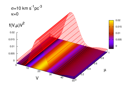
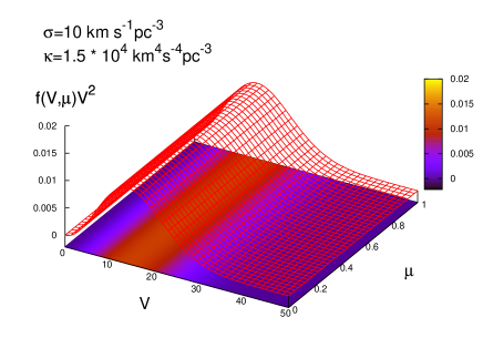
Figure 2: left: VDF where $\sigma=10\text{km}\,\text{s}^{-1}\text{pc}^{-3}$, the remaining moments and anisotropy parameters are set zero. right: VDF where $\sigma=10\text{km}\,\text{s}^{-1}\text{pc}^{-3}$, $\kappa=15\rho\sigma^{4}$, the remaining moments and anisotropy parameters are set zero. The right plot shows the MB distribution in thermal equilibrium

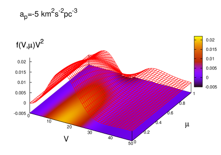
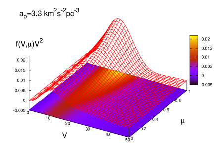
Figure 3: VDF with two different values for the anisotropy $a_{p}$. left: Shows the effect of negative anisotropy $a_{p}$ on a MB distribution. right: Shows the effect of positive anisotropy $a_{p}$ on a MB distribution.

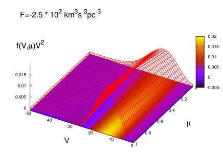
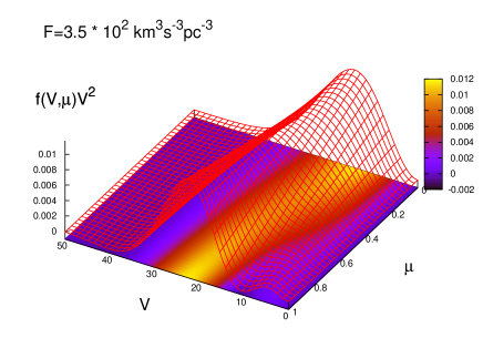
Figure 4: VDF with two different values for the third order total moment $F$ corresponding to energy flux. left: Shows the effect of negative $F$ on a MB distribution. right: The effect of positive $F$ on a MB distribution

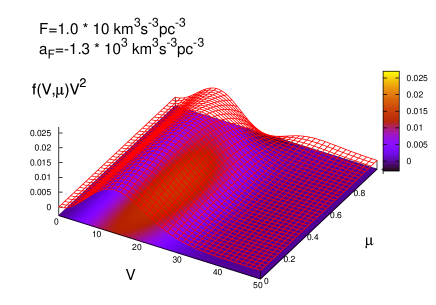
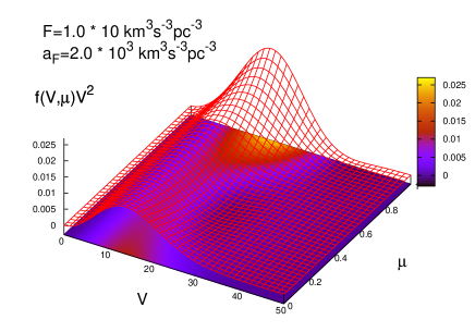
Figure 5: VDF with two different values for the third order anisotropy $a_{F}$. left: Shows the effect of negative anisotropy $a_{F}$ on the VDF. right: The effect of positive anisotropy $a_{F}$ on the VDF.

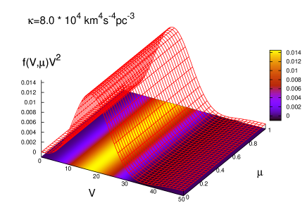
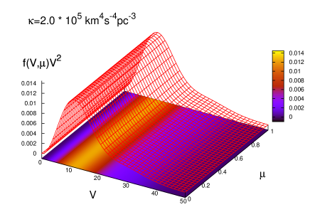
Figure 6: VDF with two different values for the total moments $\kappa$. left: VDF with lower value for $\kappa$ with respect to the MB distribution. right: VDF with higher value for $\kappa$ with respect to the MB distribution.

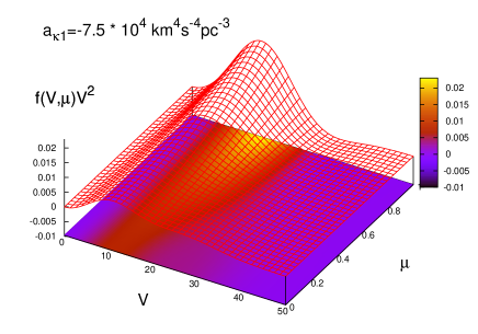
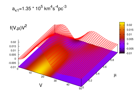
Figure 7: VDF with two different values for the fourth order anisotropy $a_{\kappa 1}$. left: The effect of negative anisotropy $a_{\kappa 1}$ on a MB distribution. right: The effect of a positive anisotropy $a_{\kappa 1}$ on a MB distribution

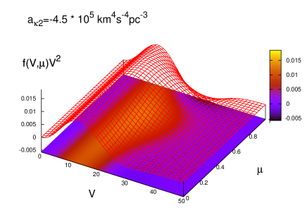
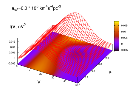
Figure 8: VDF with two different values for the fourth order anisotropy $a_{\kappa 2}$. left: The effect of negative anisotropy $a_{\kappa 2}$ on a MB distribution. right: The effect of of anisotropy $a_{\kappa 2}$ on a MB distribution

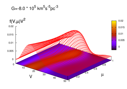
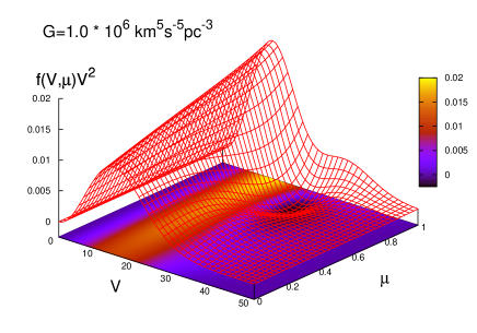
Figure 9: VDF with two different values for the total moment $G$. left: Shows the effect of negative $G$ on a MB distribution. right: Shows the effect of positive $G$ on a MB distribution

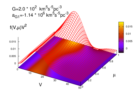
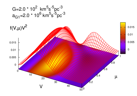
Figure 10: VDF with two different values for the fifth order anisotropy $a_{G1}$. left column: Shows the effect of negative anisotropy $a_{G1}$ on the VDF. right column: Shows the effect of positive anisotropy $a_{G1}$ on the VDF.

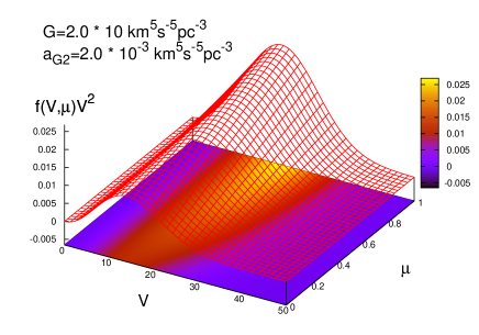
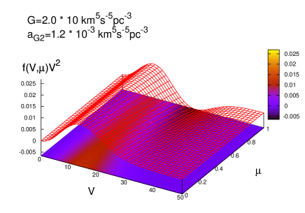
Figure 11: VDF with two different values for the fifth order anisotropy $a_{G2}$. left: Shows the effect of negative anisotropy $a_{G2}$ on the VDF. right: The effect of positive anisotropy $a_{G2}$ on the VDF.

The anisotropy $a_{p}$ describes the difference between the second order moments $p_{r}$ and $p_{t}$ which represent the radial and tangential pressure (or equivalently energy density) respectively. In thermal equilibrium we have $p_{r}=p_{t}$ and thus $a_{p}=0$. The second order moments determine the width of the VDF given by the dispersion $\sigma$. When the anisotropy $a_{p}<0$ the tangential pressure exceeds the radial pressure. As a consequence, we observe in the left plot of figure 3 that for $\mu\rightarrow 1$ the number of particles decreases whereas for $\mu\rightarrow 0$ the number of particles increases. Since $\mu$ determines the fraction of the radial and tangential velocity component this physically means that we have more particles with circular orbits when $a_{p}<0$. For $a_{p}>0$ we have the opposite behavior.

A very similar effect is caused by the fourth order anisotropy $a_{\kappa 1}$ as can be seen in figure 7. It appears together with $P_{2}(\mu)$ and the same powers of $V$ as $a_{p}$. However, since $a_{\kappa 1}$ and $a_{p}$ appear with a different sign they have opposite effects. Consequently, we can assume that the fourth order anisotropy $a_{\kappa 1}$ is a correction of the second order anisotropy $a_{p}$.

The same argument holds for the third order anisotropy $a_{F}$ (figure 5) and fifth order anisotropy $a_{G1}$ (figure 10). Both appear as factors of the Legendre polynomial $P_{3}(\mu)$ with the same powers of $V$, but different sign. Thus $a_{G1}$ can be seen as a correction of the third order anisotropy $a_{F}$.

In equation (LABEL:distr) we observe that uneven moments appear with uneven Legendre polynomials $P_{l}(\mu)$. However, these Legendre polynomials vanish at $\mu=0$ and thus the VDF is independent on uneven moments at $\mu=0$. In other words, since $\mu=0$ corresponds to stars that have a vanishing radial velocity component $v_{r}$, the distribution of stars that move on circular orbits are not affected by third order moments. This effect can be seen in in figures 4, 5, 9, 10 and 11.

When including third order moments the VDF depends on the total moment $F$ and the anisotropy $a_{F}$, where $F$ is related to the total energy flux and $a_{F}$ describes differences between radial and tangential energy fluxes. Negative values of the total moment $F$ result in an increase of the maximum of the VDF for $\mu\rightarrow 1$ (figure 4, left plot). We thus find more stars with eccentric orbits for $F<0$. When $F>0$ the maximum of the VDF shifts to higher velocities $V$ when $\mu\rightarrow 1$ (figure 4, right plot). This means that positive $F$ increases the radial velocity component $v_{r}$, but leaves the tangential component constant. As a consequence it increases the eccentricity of orbits, but not the number of stars with eccentric orbits as it does for $F<0$. Note that the two plots in figure 4 have different scaling in the $z$-axis with respect to each other in order to display the distinct effects for $F<0$ and $F>0$. Whereas the maximum of the VDF changes for $F<0$ from $\approx 0.01\text{pc}^{-3}(\text{km/s})^{-3}$ at $\mu=0$ to $\approx 0.015\text{pc}^{-3}(\text{km/s})^{-3}$ at $\mu=1$ in the left plot of figure 4 it roughly stays constant for all values of $\mu$ in the right plot corresponding to $F>0$. The effect of the third order anisotropy $a_{F}$ is displayed in figure 5. $a_{F}<0$ increases the number of stars with velocities above the mean and directions corresponding to $\mu\approx 0.5$ whereas $a_{F}>0$ causes an inverse effect.

The fourth order moments are related to the kurtosis of the velocity distribution which gives a measure of high velocity stars as compared to thermal equilibrium. In figure 6 the VDF is plotted for two different values of the total moment of fourth order $\kappa$. In the left plot $\kappa$ is chosen to be smaller than $15\rho\sigma^{4}$. The VDF increases at its mean at the expense of high and low velocities. This corresponds to a deficiency of stars with high or low velocities but more stars with velocities near the mean, compared to thermal equilibrium. In the right plot the value of $\kappa$ is chosen to be higher than $15\rho\sigma^{4}$. The wing of the VDF towards high velocities becomes thicker whereas the maximum of the VDF is smaller when compared to thermal equilibrium. Here the number of high velocity stars increases at the expense of stars with intermediate velocities.

Whereas the anisotropy $a_{\kappa 1}$ should be viewed in combination with the second order anisotropy $a_{p}$ as mentioned before, the anisotropy $a_{\kappa 2}$ gives a new characterization of anisotropy at fourth order, which is displayed in figure 8.

The effect of the total moment $G$ on the VDF is illustrated in figure 9. To get a physical understanding of this quantity we compare it to the total moment of third order $F$. $F$ is an uneven moment which was considered to denote the radial flux of random kinetic energy. The random kinetic energy density $e$ was given by the second order moments as $e=(p_{r}+2p_{t})/2$. Thus the third order moment $F$ is the corresponding flux quantity for the second order moment $p$. Equivalently we can relate the fifth order moment $G$ and the fourth order moment $\kappa$. Since $\kappa$ is related to the number of high velocity stars $G$ can be considered as a measure for the flux of these stars. Again $a_{G1}$ (figure 10) should be viewed in the context of the third order anisotropy $a_{F}$ whereas $a_{G2}$ (figure 10) determines a new type of anisotropy at fifth order.

Thus, every moment and anisotropy parameter has its own affect on the VDF. They act on different velocity intervals and redistribute stars from distinct orbitals. If we only include moments up to third order into our model, as it has been done in previous studies, our VDF is strongly limited. We are then not able to describe areas in velocity space as is possible with moments of order $>3$. More precisely, we obtain a much more detailed description of the distribution of stars in velocity space for stars with high velocities and stars which have neither radial nor tangential orbits, i.e. $0<\mu<1$.

8 Discussion

In this work we develop two statistical moment models for dense stellar dynamical systems. They are closed either at fifth- or at sixth-order depending on the required accuracy. They describe in a self-consistent way (including Fokker-Planck relaxation terms) local deviations of the velocity distribution function from the MB distribution. The description of the velocity distribution function includes third- and fourth-order moments. Third-order moments represent energy fluxes equivalent to asymmetries of the velocity distribution around its center. Fourth order moments denote deviations from the MB distribution at high velocities. This cannot be described by a velocity distribution that is fully determined by its first two moments such as a Gaussian, commonly used to fit observational data. Due to the larger number of moments of the velocity distribution, the two models we introduce have the potential to fit detailed star-star and integrated light observations of globular clusters or nuclear star clusters in detail. However, they still underly a number of approximations, such as assuming spherical symmetry, equal stellar masses, the Fokker-Planck and the local approximation and they also require a system with a high number of stars or high star densities so as to justify the statistical treatment. As the model equations only account for two-body relaxation, other mechanisms that drive the evolution of a stellar system can be added as terms in the model equations later on (e.g. unequal stellar masses and stellar evolution). In this work we have focused on giving the first complete analytical derivation of the relevant high-order moment equations.

One of our goals is also to improve previous models such as the AGM or the moment model of Louis (1990). For that, we achieve a more accurate modeling by including a larger number of moments. As we explained in section 7, increasing the number of moments leads to both a more complex VDF and an increasing number of differential moment equations (section 4.1). This argument applies to the AGM rather than Louis’ model.

We therefore can describe the state of the system in terms of its phase space distribution function more accurately. As explained previously, GCs are in dynamic equilibrium but not in thermodynamic equilibrium. While a system in thermodynamic equilibrium can be represented by a VDF that is fully defined by its first two moments, the number of non-vanishing moments increases for a system which is not in thermodynamic equilibrium. In most cases, it is impossible to exactly compute the VDF for a system that is not in thermodynamic equilibrium. In a stellar dynamical system such as GCs or NCs there are numerous mechanisms that force the system away from thermodynamic equilibrium, raising the issue of when to truncate the moment series. Mechanisms that affect the high end of the VDF, such as the evaporation of stars from a stellar system, close three-body encounters and mass-segregation, suggest that the inclusion of fourth- and fifth- order moments are important. This is also fortified by observations such as in the findings of high velocity stars in the core of Milky Way GCs. The AGM, as a 3rd order model, does not accurately describe these mechanisms.

The correct computation of the collisional terms is still a major difficulty and the local approximation is applied and an ansatz for the VDF is used to handle this problem. Even so, there are evident improvements over the previous models that stem from the use of a larger number of moments (regarding the AGM) and a self-consistent method for the computation of the collisional terms (as compared to Louis 1990). In contrast to the previous models, the collision term of a moment equation of order $n$ does not only depend on the corresponding $n$th order anisotropy parameter but instead exhibits more dependencies on anisotropy of the parameters and moments of almost all orders as well. This leads to further coupling between the different moments. In a comparative study between the AGM and FP and $N$-body models, Spurzem & Takahashi (1995) concluded that in a multi-mass model a significant fraction of small-angle encounters, which transfer energy from the heavy to the light stars in the core, cause the light stars to move radially outwards on elongated orbits. As a result, the energy taken from the heavy particles is quickly redistributed over a much larger volume than assumed by the local approximation. Even though the local approximation is still applied in this model, the energy transfer due to collisions should be improved due to a stronger coupling of the moments. This will provide a better estimate for the impact of the local approximation of the evolution of the system.

The choice of the closure relation is very important, in particular at lower orders. In the AGM the system of equations is closed with the heat flux equation, which relates the energy flux to the velocity dispersion. It is not clear how well the heat conduction closure of the AGM works. It obviously allows the model to handle heat transfer and there are certainly parallels to gas-dynamics in GCs, but the description of energy transfer via the gas-dynamical heat conduction equation might nevertheless be a too simple description of this process. The heat conduction closure and the third order differential moment equations seems to be two completely different descriptions of a similar process. Even so, in the comparative study by Louis & Spurzem (1991) between the AGM and the model of Louis (1990) reasonable agreement in pre-core-collapse could be achieved by proper choice of the free parameters of the AGM. However, these values of the free parameters of the AGM are not in agreement with the values resulting from the comparative study by Giersz & Spurzem (1994), where the AGM was fitted and compared to FP and $N$-body models. This indicates that Louis’ model does not agree very well with FP and $N$-body models. Furthermore, it has to be considered that the parameter $\lambda$ determining the heat conduction in gaseous models is just a scaling factor in isotropic gaseous models. In anisotropic gaseous models $\lambda$ prescribes the relative speed of the two relevant processes - the decay of anisotropy and the heat flow between warm and cold regions. With growing $\lambda$ heat flows faster, so there is less time for gravitational encounters to destroy anisotropy (Louis & Spurzem 1991). In our model (as in the model of Louis (1990)) this free parameter is absent.

The closure equation in the model of Louis (1990) is an algebraic relation between the flux velocities of even moments $\kappa$, $p$ and $\rho$. It is based on the assumption that the flux velocities of moments of order 2k increase with k.

The closure relations we use are basically a mathematical formulation of the fact that our model cannot describe an arbitrary degree of anisotropy, since its description of a stellar system is bounded by the highest moment that it includes. It also reflects the limits of variability of the VDF and, thus, is a very natural choice. The only uncertainty of this closure relation is the error due to the polynomial ansatz for the VDF. The closure limiting the VDF is derived from the VDF itself. It does not stem from any other constraint that is independent of the form of the VDF arising from the boundary conditions like spherical symmetry and the absence of rotation. Hence, this ansatz should not be seen as an additional approximation, but rather as a consistency relation.

The model equations consist of the set of equations (LABEL:moment_equations_a) and (LABEL:moment_equations_b) for model a where the right-hand sides are given by equations (LABEL:begin_fourth_order) to (LABEL:end_fourth_order) and the set of equations (LABEL:moment_equations_a), (LABEL:moment_equations_b) and (LABEL:moment_equations_c) for model b with the right-hand sides given in equations (LABEL:begin_fifth_order) to (LABEL:end_fifth_order). Furthermore, we need the Poisson equation (25) and the closure relations (39) or (LABEL:Hrelations) to complete the model equations. In order to exclude errors in the computation of the collisional terms, several measures were taken. The higher order Rosenbluth potentials were compared to the second-order Rosenbluth potentials of Giersz & Spurzem (1994) and showed exact agreement. Furthermore, the collisional terms for the density, bulk velocity and energy density vanish as expected according to mass and energy conservation and the fact that internal collisions do not disturb the motion of the barycenter.

Eventually, several arguments have been given that predict improvements of the fourth and fifth order models developed in this work in comparison with its predecessors but a final estimate of the gained accuracy can only be obtained by means of numerical simulations and subsequent comparison with other models. The next step will be to implement and test the model in a numerical code such as the anisotropic gaseous model. For that, the left-hand sides of the differential moment equations (LABEL:moment_equations_a), (LABEL:moment_equations_b) and (LABEL:moment_equations_c) have to be discretized as in the appendix of Amaro-Seoane et al. (2004), and the collisional terms which form the right-hand sides of the moment equations have to be reformulated. They should be simplified and reordered to allow an effective implementation into a numerical code.

Appendix A Collisional terms

$$\begin{split}&\left(\frac{\delta p_{r}}{\delta t}\right)_{\text{enc}}=-2\left(\frac{\delta p_{t}}{\delta t}\right)_{\text{enc}}=\frac{1}{t_{\mathrm{rx}}}\bigg{(}-\frac{177a_{p}}{640}\\ &+\frac{1}{\rho\sigma^{2}}\bigg{(}\frac{39a_{p}^{2}}{160}-\frac{27\rho a_{\text{$\kappa$1}}}{8960}+\frac{1}{\rho\sigma^{2}}\bigg{(}\frac{9F^{2}}{100}+\frac{27Fa_{F}}{1400}\\ &+\frac{a_{F}^{2}}{1400}-\frac{33\kappa a_{p}}{640}-\frac{33a_{p}a_{\text{$\kappa$1}}}{1568}-\frac{33a_{p}a_{\text{$\kappa$2}}}{15680}\\ &+\frac{1}{\rho\sigma^{2}}\bigg{(}\frac{3a_{\text{$\kappa$1}}^{2}}{6272}+\frac{3\kappa a_{\text{$\kappa$1}}}{1280}+\frac{3a_{\text{$\kappa$1}}a_{\text{$\kappa$2}}}{31360}+\frac{a_{\text{$\kappa$2}}^{2}}{413952}\bigg{)}\bigg{)}\bigg{)}\bigg{)}\end{split}$$ (76)

$$\begin{split}&\left(\frac{\delta F_{r}}{\delta t}\right)_{\text{enc}}=\frac{1}{t_{\mathrm{rx}}}\bigg{(}-\frac{423F}{400}-\frac{4833a_{F}}{22400}\\ &+\frac{1}{\rho\sigma^{2}}\bigg{(}\frac{9Fa_{p}}{112}-\frac{9a_{F}a_{p}}{280}+\frac{1}{\rho\sigma^{2}}\bigg{(}\frac{9F\kappa}{400}-\frac{81\kappa a_{F}}{22400}\\ &+\frac{9Fa_{\text{$\kappa$1}}}{1120}+\frac{9a_{F}a_{\text{$\kappa$1}}}{3920}+\frac{9Fa_{\text{$\kappa$2}}}{2800}-\frac{3a_{F}a_{\text{$\kappa$2}}}{78400}\bigg{)}\bigg{)}\bigg{)}\end{split}$$ (77)

$$\begin{split}&\left(\frac{\delta F_{t}}{\delta t}\right)_{\text{enc}}=\frac{1}{t_{\mathrm{rx}}}\bigg{(}-\frac{141F}{200}+\frac{4833a_{F}}{22400}\\ &+\frac{1}{\rho\sigma^{2}}\bigg{(}\frac{1203Fa_{p}}{2800}-\frac{81a_{F}a_{p}}{1400}+\frac{1}{\rho\sigma^{2}}\bigg{(}\frac{3F\kappa}{200}\\ &+\frac{81\kappa a_{F}}{22400}-\frac{3Fa_{\text{$\kappa$1}}}{160}+\frac{9a_{F}a_{\text{$\kappa$1}}}{3920}-\frac{9Fa_{\text{$\kappa$2}}}{2800}\\ &-\frac{17a_{F}a_{\text{$\kappa$2}}}{78400}\bigg{)}\bigg{)}\bigg{)}\end{split}$$ (78)

$$\begin{split}&\left(\frac{\delta\kappa_{r}}{\delta t}\right)_{\text{enc}}=\frac{1}{t_{\mathrm{rx}}}\bigg{(}-\frac{93\kappa}{400}-\frac{18069a_{\text{$\kappa$1}}}{62720}\\ &-\frac{6773a_{\text{$\kappa$2}}}{156800}+\frac{31a_{p}^{2}}{32\rho}+\sigma^{2}\bigg{(}\frac{11481a_{p}}{4480}+\frac{423\rho\sigma^{2}}{160}\bigg{)}\\ &+\frac{1}{\rho\sigma^{2}}\bigg{(}-\frac{2697a_{p}a_{\text{$\kappa$2}}}{123200}+\frac{1593F^{2}}{3500}+\frac{1257Fa_{F}}{7000}\\ &+\frac{81a_{F}^{2}}{77000}-\frac{111a_{p}a_{\text{$\kappa$1}}}{1120}-\frac{789\kappa a_{p}}{3200}+\frac{1}{\rho\sigma^{2}}\bigg{(}\frac{129a_{\text{$\kappa$1}}^{2}}{43904}\\ &+\frac{699\kappa a_{\text{$\kappa$1}}}{62720}+\frac{3\kappa^{2}}{800}-\frac{37\kappa a_{\text{$\kappa$2}}}{156800}+\frac{2567a_{\text{$\kappa$1}}a_{\text{$\kappa$2}}}{2414720}\\ &-\frac{181a_{\text{$\kappa$2}}^{2}}{313913600}\bigg{)}\bigg{)}\bigg{)}\end{split}$$ (79)

$$\begin{split}&\left(\frac{\delta\kappa_{rt}}{\delta t}\right)_{\text{enc}}=\frac{1}{t_{\mathrm{rx}}}\bigg{(}-\frac{31\kappa}{200}-\frac{6023a_{\text{$\kappa$1}}}{125440}\\ &+\frac{6773a_{\text{$\kappa$2}}}{156800}-\frac{647a_{p}^{2}}{1344\rho}+\sigma^{2}\bigg{(}\frac{3827a_{p}}{8960}+\frac{141\rho\sigma^{2}}{80}\bigg{)}\\ &+\frac{1}{\rho\sigma^{2}}\bigg{(}-\frac{263\kappa a_{p}}{6400}+\frac{509a_{p}a_{\text{$\kappa$1}}}{15680}-\frac{6693a_{p}a_{\text{$\kappa$2}}}{1724800}\\ &+\frac{39Fa_{F}}{2800}-\frac{3a_{F}^{2}}{880}+\frac{207F^{2}}{1400}+\frac{1}{\rho\sigma^{2}}\bigg{(}\frac{233\kappa a_{\text{$\kappa$1}}}{125440}\\ &+\frac{\kappa^{2}}{400}+\frac{37\kappa a_{\text{$\kappa$2}}}{156800}-\frac{53a_{\text{$\kappa$1}}^{2}}{87808}+\frac{509a_{\text{$\kappa$1}}a_{\text{$\kappa$2}}}{4829440}\\ &-\frac{28879a_{\text{$\kappa$2}}^{2}}{1883481600}\bigg{)}\bigg{)}\bigg{)}\end{split}$$ (80)

$$\begin{split}&\left(\frac{\delta\kappa_{t}}{\delta t}\right)_{\text{enc}}=\frac{1}{t_{\mathrm{rx}}}\bigg{(}-\frac{31\kappa}{50}+\frac{6023a_{\text{$\kappa$1}}}{15680}\\ &-\frac{6773a_{\text{$\kappa$2}}}{156800}-\frac{53a_{p}^{2}}{84\rho}+\sigma^{2}\bigg{(}-\frac{3827a_{p}}{1120}+\frac{141\rho\sigma^{2}}{20}\bigg{)}\\ &+\frac{1}{\rho\sigma^{2}}\bigg{(}\frac{263\kappa a_{p}}{800}+\frac{6393a_{p}a_{\text{$\kappa$2}}}{215600}+\frac{23a_{p}a_{\text{$\kappa$1}}}{980}-\frac{39a_{F}^{2}}{5500}\\ &-\frac{27F^{2}}{875}-\frac{363Fa_{F}}{1750}+\frac{1}{\rho\sigma^{2}}\bigg{(}\frac{\kappa^{2}}{100}+\frac{a_{\text{$\kappa$1}}^{2}}{5488}-\frac{233\kappa a_{\text{$\kappa$1}}}{15680}\\ &-\frac{37\kappa a_{\text{$\kappa$2}}}{156800}-\frac{769a_{\text{$\kappa$1}}a_{\text{$\kappa$2}}}{603680}-\frac{15319a_{\text{$\kappa$2}}^{2}}{470870400}\bigg{)}\bigg{)}\bigg{)}\end{split}$$ (81)

And the collisional terms for the model closing at sixth order are:

$$\begin{split}&\left(\frac{\delta p_{r}}{\delta t}\right)_{\text{enc}}=-2\left(\frac{\delta p_{t}}{\delta t}\right)_{\text{enc}}=\frac{1}{t_{\text{rx}}}\bigg{(}-\frac{177a_{p}}{640}\\ &+\frac{1}{\rho\sigma^{2}}\bigg{(}\frac{39a_{p}^{2}}{160}-\frac{27\rho a_{\text{$\kappa$1}}}{8960}+\frac{1}{\rho\sigma^{2}}\bigg{(}\frac{243F^{2}}{320}\\ &+\frac{729Fa_{F}}{4480}+\frac{27a_{F}^{2}}{4480}-\frac{33a_{p}a_{\text{$\kappa$2}}}{15680}-\frac{33\kappa a_{p}}{640}-\frac{33a_{p}a_{\text{$\kappa$1}}}{1568}\\ &+\frac{1}{\rho\sigma^{2}}\bigg{(}\frac{3\kappa a_{\text{$\kappa$1}}}{1280}-\frac{39Fa_{\text{G1}}}{3200}-\frac{13a_{F}a_{\text{G1}}}{14400}-\frac{13a_{F}a_{\text{G2}}}{177408}\\ &+\frac{3a_{\text{$\kappa$1}}^{2}}{6272}-\frac{117FG}{3200}-\frac{351Ga_{F}}{89600}+\frac{3a_{\text{$\kappa$1}}a_{\text{$\kappa$2}}}{31360}+\frac{a_{\text{$\kappa$2}}^{2}}{413952}\\ &+\frac{1}{\rho\sigma^{2}}\bigg{(}\frac{a_{\text{G1}}a_{\text{G2}}}{177408}+\frac{a_{\text{G2}}^{2}}{9225216}+\frac{a_{\text{G1}}^{2}}{28800}+\frac{27Ga_{\text{G1}}}{89600}\\ &+\frac{81G^{2}}{179200}\bigg{)}\bigg{)}\bigg{)}\bigg{)}\bigg{)}\end{split}$$ (82)

$$\begin{split}&\left(\frac{\delta F_{r}}{\delta t}\right)_{\text{enc}}=\frac{1}{t_{\text{rx}}}\bigg{(}-\frac{171F}{80}-\frac{5697a_{F}}{17920}\\ &+\frac{1}{\rho\sigma^{2}}\bigg{(}\frac{1017\rho a_{\text{G1}}}{89600}+\frac{27\rho G}{700}+\frac{351Fa_{p}}{320}\\ &+\frac{1}{\rho\sigma^{2}}\bigg{(}\frac{9F\kappa}{400}-\frac{1269\kappa a_{F}}{89600}-\frac{2277Ga_{p}}{62720}\\ &-\frac{a_{\text{G1}}a_{p}}{280}-\frac{107a_{\text{G2}}a_{p}}{68992}-\frac{99Fa_{\text{$\kappa$1}}}{4480}+\frac{9a_{F}a_{\text{$\kappa$1}}}{3920}\\ &+\frac{81Fa_{\text{$\kappa$2}}}{11200}-\frac{1357a_{F}a_{\text{$\kappa$2}}}{3449600}+\frac{1}{\rho\sigma^{2}}\bigg{(}\frac{3\kappa a_{\text{G1}}}{2560}\\ &+\frac{27Ga_{\text{$\kappa$1}}}{25088}+\frac{9a_{\text{G2}}a_{\text{$\kappa$1}}}{137984}-\frac{9Ga_{\text{$\kappa$2}}}{62720}+\frac{a_{\text{G1}}a_{\text{$\kappa$2}}}{25344}\\ &-\frac{a_{\text{G2}}a_{\text{$\kappa$2}}}{1241856}\bigg{)}\bigg{)}\bigg{)}\bigg{)}\end{split}$$ (83)

$$\begin{split}&\left(\frac{\delta F_{t}}{\delta t}\right)_{\text{enc}}=\frac{1}{t_{\text{rx}}}\bigg{(}-\frac{57F}{40}+\frac{5697a_{F}}{17920}\\ &+\frac{1}{\rho\sigma^{2}}\bigg{(}\frac{9\text{$\rho$G}}{350}-\frac{1017\text{$\rho$a}_{\text{G1}}}{89600}+\frac{1521Fa_{p}}{1600}-\frac{117a_{F}a_{p}}{800}\\ &+\frac{1}{\rho\sigma^{2}}\bigg{(}\frac{3F\kappa}{200}+\frac{1269\kappa a_{F}}{89600}-\frac{1167Ga_{p}}{62720}+\frac{11a_{\text{G1}}a_{p}}{1120}\\ &+\frac{107a_{\text{G2}}a_{p}}{68992}-\frac{201Fa_{\text{$\kappa$1}}}{4480}+\frac{99a_{F}a_{\text{$\kappa$1}}}{15680}-\frac{81Fa_{\text{$\kappa$2}}}{11200}\\ &-\frac{6269a_{F}a_{\text{$\kappa$2}}}{10348800}+\frac{1}{\rho\sigma^{2}}\bigg{(}\frac{117Ga_{\text{$\kappa$1}}}{125440}-\frac{3\kappa a_{\text{G1}}}{2560}-\frac{a_{\text{G1}}a_{\text{$\kappa$1}}}{2240}\\ &-\frac{9a_{\text{G2}}a_{\text{$\kappa$1}}}{137984}+\frac{9Ga_{\text{$\kappa$2}}}{62720}+\frac{23a_{\text{G1}}a_{\text{$\kappa$2}}}{532224}-\frac{a_{\text{G2}}a_{\text{$\kappa$2}}}{338688}\bigg{)}\bigg{)}\bigg{)}\bigg{)}\end{split}$$ (84)

$$\begin{split}&\left(\frac{\delta\kappa_{r}}{\delta t}\right)_{\text{enc}}=\frac{1}{t_{\text{rx}}}\bigg{(}-\frac{93\kappa}{400}-\frac{18069a_{\text{$\kappa$1}}}{62720}-\frac{6773a_{\text{$\kappa$2}}}{156800}\\ &+\frac{31a_{p}^{2}}{32\rho}+\sigma^{2}\bigg{(}\frac{423\rho\sigma^{2}}{160}+\frac{11481\text{ }a_{p}}{4480}\bigg{)}\\ &+\frac{1}{\rho\sigma^{2}}\bigg{(}\frac{27189F^{2}}{8000}-\frac{111a_{p}a_{\text{$\kappa$1}}}{1120}-\frac{2697a_{p}a_{\text{$\kappa$2}}}{123200}\\ &+\frac{18861Fa_{F}}{16000}+\frac{2713a_{F}^{2}}{176000}-\frac{789\kappa a_{p}}{3200}+\frac{1}{\rho\sigma^{2}}\bigg{(}\frac{3\kappa^{2}}{800}\\ &-\frac{5319FG}{31360}-\frac{537Ga_{F}}{17920}-\frac{1061Fa_{\text{G1}}}{13440}-\frac{643a_{F}a_{\text{G1}}}{221760}\\ &+\frac{1499Fa_{\text{G2}}}{517440}-\frac{139a_{F}a_{\text{G2}}}{149760}+\frac{699\kappa a_{\text{$\kappa$1}}}{62720}+\frac{129a_{\text{$\kappa$1}}^{2}}{43904}\\ &-\frac{37\kappa a_{\text{$\kappa$2}}}{156800}+\frac{2567a_{\text{$\kappa$1}}a_{\text{$\kappa$2}}}{2414720}-\frac{181a_{\text{$\kappa$2}}^{2}}{313913600}\\ &+\frac{1}{\rho\sigma^{2}}\bigg{(}\frac{2889G^{2}}{1254400}+\frac{587Ga_{\text{G1}}}{268800}+\frac{413a_{\text{G1}}^{2}}{2851200}\\ &-\frac{97Ga_{\text{G2}}}{2069760}+\frac{7643a_{\text{G1}}a_{\text{G2}}}{103783680}-\frac{53a_{\text{G2}}^{2}}{264176640}\bigg{)}\bigg{)}\bigg{)}\bigg{)}\end{split}$$ (85)

$$\begin{split}&\left(\frac{\delta\kappa_{rt}}{\delta t}\right)_{\text{enc}}=\frac{1}{t_{\text{rx}}}\bigg{(}-\frac{31\kappa}{200}-\frac{6023a_{\text{$\kappa$1}}}{125440}\\ &+\frac{6773a_{\text{$\kappa$2}}}{156800}-\frac{647a_{p}^{2}}{1344\rho}+\sigma^{2}\bigg{(}\frac{141\rho\sigma^{2}}{80}+\frac{3827a_{p}}{8960}\bigg{)}\\ &+\frac{1}{\rho\sigma^{2}}\bigg{(}\frac{3627F^{2}}{3200}+\frac{291Fa_{F}}{6400}-\frac{3799a_{F}^{2}}{211200}-\frac{263\kappa a_{p}}{6400}\\ &+\frac{509a_{p}a_{\text{$\kappa$1}}}{15680}-\frac{6693a_{p}a_{\text{$\kappa$2}}}{1724800}+\frac{1}{\rho\sigma^{2}}\bigg{(}-\frac{17937FG}{313600}\\ &+\frac{\kappa^{2}}{400}+\frac{807Ga_{F}}{1254400}-\frac{691Fa_{\text{G1}}}{134400}+\frac{2179a_{F}a_{\text{G1}}}{950400}\\ &-\frac{1499Fa_{\text{G2}}}{517440}-\frac{67289a_{F}a_{\text{G2}}}{484323840}+\frac{233\kappa a_{\text{$\kappa$1}}}{125440}-\frac{53a_{\text{$\kappa$1}}^{2}}{87808}\\ &+\frac{37\kappa a_{\text{$\kappa$2}}}{156800}+\frac{509a_{\text{$\kappa$1}}a_{\text{$\kappa$2}}}{4829440}-\frac{28879a_{\text{$\kappa$2}}^{2}}{1883481600}\\ &+\frac{1}{\rho\sigma^{2}}\bigg{(}\frac{1971G^{2}}{2508800}-\frac{14947a_{\text{G2}}^{2}}{17435658240}+\frac{701a_{\text{G1}}a_{\text{G2}}}{88957440}\\ &-\frac{Ga_{\text{G1}}}{76800}+\frac{97Ga_{\text{G2}}}{2069760}-\frac{1279a_{\text{G1}}^{2}}{17107200}\bigg{)}\bigg{)}\bigg{)}\bigg{)}\end{split}$$ (86)

$$\begin{split}&\left(\frac{\delta\kappa_{t}}{\delta t}\right)_{\text{enc}}=\frac{1}{t_{\text{rx}}}\bigg{(}-\frac{31\kappa}{50}+\frac{6023a_{\text{$\kappa$1}}}{15680}-\frac{6773a_{\text{$\kappa$2}}}{156800}\\ &-\frac{53a_{p}^{2}}{84\rho}+\sigma^{2}\bigg{(}\frac{141\rho\sigma^{2}}{20}-\frac{3827a_{p}}{1120}\bigg{)}+\frac{1}{\rho\sigma^{2}}\bigg{(}\frac{9F^{2}}{2000}\\ &-\frac{5079Fa_{F}}{4000}-\frac{8927a_{F}^{2}}{264000}+\frac{263\kappa a_{p}}{800}+\frac{23a_{p}a_{\text{$\kappa$1}}}{980}\\ &+\frac{6393a_{p}a_{\text{$\kappa$2}}}{215600}+\frac{1}{\rho\sigma^{2}}\bigg{(}\frac{\kappa^{2}}{100}-\frac{207FG}{39200}+\frac{4497Ga_{F}}{156800}\\ &+\frac{1499Fa_{\text{G1}}}{16800}+\frac{943a_{F}a_{\text{G1}}}{237600}+\frac{1499Fa_{\text{G2}}}{517440}\\ &-\frac{233\kappa a_{\text{$\kappa$1}}}{15680}+\frac{73013a_{F}a_{\text{G2}}}{60540480}+\frac{a_{\text{$\kappa$1}}^{2}}{5488}-\frac{37\kappa a_{\text{$\kappa$2}}}{156800}\\ &-\frac{769a_{\text{$\kappa$1}}a_{\text{$\kappa$2}}}{603680}-\frac{15319a_{\text{$\kappa$2}}^{2}}{470870400}+\frac{1}{\rho\sigma^{2}}\bigg{(}\frac{9G^{2}}{62720}\\ &-\frac{29Ga_{\text{G1}}}{13440}-\frac{19a_{\text{G1}}^{2}}{171072}-\frac{97Ga_{\text{G2}}}{2069760}-\frac{6959a_{\text{G1}}a_{\text{G2}}}{77837760}\\ &-\frac{251a_{\text{G2}}^{2}}{136216080}\bigg{)}\bigg{)}\bigg{)}\bigg{)}\end{split}$$ (87)

$$\begin{split}&\left(\frac{\delta G_{r}}{\delta t}\right)_{\text{enc}}=\frac{1}{t_{\text{rx}}}\bigg{(}-\frac{25009a_{\text{G1}}}{161280}-\frac{35521a_{\text{G2}}}{1241856}\\ &+\frac{a_{p}}{\rho}\bigg{(}\frac{3231F}{448}+\frac{a_{F}}{168}\bigg{)}-\sigma^{2}\bigg{(}\frac{1683F}{560}+\frac{1013a_{F}}{2560}\bigg{)}\\ &-\frac{1161G}{7840}+\frac{1}{\rho\sigma^{2}}\bigg{(}-\frac{351F\kappa}{2800}-\frac{8207\kappa a_{F}}{89600}\\ &-\frac{16119Ga_{p}}{62720}-\frac{181a_{\text{G1}}a_{p}}{3465}-\frac{45Fa_{\text{$\kappa$1}}}{896}+\frac{59a_{F}a_{\text{$\kappa$1}}}{4312}\\ &-\frac{164105a_{\text{G2}}a_{p}}{8072064}+\frac{4689Fa_{\text{$\kappa$2}}}{61600}-\frac{326083a_{F}a_{\text{$\kappa$2}}}{44844800}\\ &+\frac{1}{\rho\sigma^{2}}\bigg{(}\frac{9G\kappa}{1120}+\frac{1247\kappa a_{\text{G1}}}{161280}-\frac{\kappa a_{\text{G2}}}{25344}+\frac{1143Ga_{\text{$\kappa$1}}}{175616}\\ &+\frac{11a_{\text{G1}}a_{\text{$\kappa$1}}}{7056}+\frac{97805a_{\text{G2}}a_{\text{$\kappa$1}}}{113008896}-\frac{3303Ga_{\text{$\kappa$2}}}{2414720}\\ &+\frac{49523a_{\text{G1}}a_{\text{$\kappa$2}}}{80720640}-\frac{4027a_{\text{G2}}a_{\text{$\kappa$2}}}{113008896}\bigg{)}\bigg{)}\bigg{)}\end{split}$$ (88)

$$\begin{split}&\left(\frac{\delta G_{rt}}{\delta t}\right)_{\text{enc}}=\frac{1}{t_{\text{rx}}}\bigg{(}\frac{25009a_{\text{G1}}}{1612800}+\frac{35521a_{\text{G2}}}{1241856}\\ &+\frac{a_{p}}{\rho}\bigg{(}\frac{9669F}{4480}-\frac{3229a_{F}}{6720}\bigg{)}-\sigma^{2}\bigg{(}\frac{1683F}{1400}-\frac{1013a_{F}}{25600}\bigg{)}\\ &-\frac{1161G}{19600}+\frac{1}{\rho\sigma^{2}}\bigg{(}-\frac{351F\kappa}{7000}+\frac{8207\kappa a_{F}}{896000}-\frac{1557Ga_{p}}{25088}\\ &+\frac{5017a_{\text{G1}}a_{p}}{221760}+\frac{210101a_{\text{G2}}a_{p}}{80720640}-\frac{12573Fa_{\text{$\kappa$1}}}{313600}\\ &+\frac{34381a_{F}a_{\text{$\kappa$1}}}{1724800}-\frac{130341Fa_{\text{$\kappa$2}}}{8624000}-\frac{1572817a_{F}a_{\text{$\kappa$2}}}{448448000}\\ &+\frac{1}{\rho\sigma^{2}}\bigg{(}\frac{9G\kappa}{2800}-\frac{1247\kappa a_{\text{G1}}}{1612800}+\frac{\kappa a_{\text{G2}}}{25344}+\frac{189857a_{\text{G1}}a_{\text{$\kappa$2}}}{807206400}\\ &-\frac{311a_{\text{G1}}a_{\text{$\kappa$1}}}{282240}-\frac{4483a_{\text{G2}}a_{\text{$\kappa$1}}}{32288256}+\frac{309Ga_{\text{$\kappa$2}}}{985600}+\frac{459Ga_{\text{$\kappa$1}}}{250880}\\ &-\frac{731a_{\text{G2}}a_{\text{$\kappa$2}}}{32288256}\bigg{)}\bigg{)}\bigg{)}\end{split}$$ (89)

$$\begin{split}&\left(\frac{\delta G_{t}}{\delta t}\right)_{\text{enc}}=\frac{1}{t_{\text{rx}}}\bigg{(}-\frac{387G}{4900}+\frac{25009a_{\text{G1}}}{201600}-\frac{35521a_{\text{G2}}}{1241856}\\ &+\frac{a_{p}}{\rho}\bigg{(}\frac{1069F}{560}-\frac{533a_{F}}{1680}\bigg{)}-\sigma^{2}\bigg{(}\frac{561F}{350}-\frac{1013a_{F}}{3200}\bigg{)}\\ &+\frac{1}{\rho\sigma^{2}}\bigg{(}-\frac{117F\kappa}{1750}+\frac{8207\kappa a_{F}}{112000}-\frac{2229Ga_{p}}{78400}+\frac{2581a_{\text{G1}}a_{p}}{277200}\\ &+\frac{76303a_{\text{G2}}a_{p}}{5045040}-\frac{3141Fa_{\text{$\kappa$1}}}{39200}+\frac{5669a_{F}a_{\text{$\kappa$1}}}{431200}-\frac{197889Fa_{\text{$\kappa$2}}}{4312000}\\ &-\frac{505481a_{F}a_{\text{$\kappa$2}}}{168168000}+\frac{1}{\rho\sigma^{2}}\bigg{(}\frac{3G\kappa}{700}-\frac{1247\kappa a_{\text{G1}}}{201600}-\frac{\kappa a_{\text{G2}}}{25344}\\ &+\frac{309Ga_{\text{$\kappa$1}}}{219520}-\frac{31a_{\text{G1}}a_{\text{$\kappa$1}}}{70560}-\frac{8303a_{\text{G2}}a_{\text{$\kappa$1}}}{14126112}+\frac{17889Ga_{\text{$\kappa$2}}}{24147200}\\ &+\frac{63001a_{\text{G1}}a_{\text{$\kappa$2}}}{302702400}-\frac{3119a_{\text{G2}}a_{\text{$\kappa$2}}}{169513344}\bigg{)}\bigg{)}\bigg{)}\end{split}$$ (90)

References

• Aarseth (1999) Aarseth S. J., 1999, The Publications of the Astronomical Society of the Pacific, 111, 1333
• Amaro-Seoane (2004) Amaro-Seoane P., 2004, PhD thesis, PhD Thesis, Combined Faculties for the Natural Sciences and for Mathematics of the University of Heidelberg, Germany. VII + 159 pp. (2004), arXiv:astro-ph/0502414
• Amaro-Seoane et al. (2010) Amaro-Seoane P., Eichhorn C., Porter E. K., Spurzem R., 2010, Monthly Notices of the Royal Astronomical Society, 57, 2268
• Amaro-Seoane & Freitag (2006) Amaro-Seoane P., Freitag M., 2006, 653, L53
• Amaro-Seoane et al. (2004) Amaro-Seoane P., Freitag M., Spurzem R., 2004, Monthly Notices of the Royal Astronomical Society, 352, 655
• Amaro-Seoane et al. (2009) Amaro-Seoane P., Miller M. C., Freitag M., 2009, 692, L50
• Amaro-Seoane et al. (2001) Amaro-Seoane, P., Spurzem, R., 2001, The Central Kiloparsec of Starbursts and AGN: The La Palma Connection 249, 731
• Amaro-Seoane & Spurzem (2004) Amaro-Seoane P., Spurzem R., 2004, in In ”Carnegie Observatories Astrophysics Series, Vol. 1: Coevolution of Black Holes and Galaxies,” ed. L. C. Ho, Pasadena, USA: Carnegie Observatories
• Amaro-Seoane et al. (2002) Amaro-Seoane, P., Spurzem, R., Just, A., 2002, Lighthouses of the Universe: The Most Luminous Celestial Objects and Their Use for Cosmology 376
• Amaro-Seoane et al. (2003) Amaro-Seoane P., Spurzem R., Just A., 2003, EAS Publications Series, Volume 10, 2003, Galactic and Stellar Dynamics, Proceedings of JENAM 2002, held in Porto, Portugal, 3-6 September, 2002. Edited by C. M. Boily, P. Pastsis, S. Portegies Zwart, R. Spurzem and C. Theis, pp.189., 10, 189
• Ardi et al. (2005) Ardi E., Spurzem R., Mineshige S., 2005, Journal of the Korean Astronomical Society, 38, 207
• Begelman (2010) Begelman, M. C., 2010, Monthly Notices of the Royal Astronomical Society 402, 673
• Berentzen et al. (2009) Berentzen I., Preto M., Berczik P., Merritt D., Spurzem R., 2009, The Astrophysical Journal, 695, 455
• Bettwieser (1983) Bettwieser E., 1983, Monthly Notices of the Royal Astronomical Society, 203, 811
• Bettwieser & Spurzem (1986) Bettwieser E., Spurzem R., 1986, Astronomy and Astrophysics, 161, 102
• Bettwieser & Sugimoto (1984) Bettwieser E., Sugimoto D., 1984, Monthly Notices of the Royal Astronomical Society, 208, 493
• Bisnovatyi-Kogan & Sunyaev (1972) Bisnovatyi-Kogan G. S., Syunyaev R. A., 1972 , Astronomicheskii Zhurnal 49, 243
• Boily (2000) Boily C. M., 2000, Massive Stellar Clusters, Proceedings of the international workshop held in Strasbourg, France, November 8-11, 1999. Eds.: A. Lançon, and C. Boily, Astronomical Society of the Pacific Conference Series, 190
• Boily & Spurzem (2000) Boily C. M., Spurzem R., 2000, The Galactic Halo : From Globular Cluster to Field Stars, Proceedings of the 35th Liege International Astrophysics Colloquium, 607
• Chandrasekhar (1942) Chandrasekhar S., 1942,Principles of stellar dynamics, University of Chicago Press, 96, 160
• Chernoff & Weinberg (1990) Chernoff D. F., Weinberg M. D., 1990, Astronomical Society of Japan, 351, 121
• Ciotti et al. (2009) Ciotti, L., Ostriker, J. P., Proga, D., 2009, The Astrophysical Journal 699, 89
• Ciotti et al. (2010) Ciotti, L., Ostriker, J. P., Proga, D., 2010, ArXiv e-prints arXiv:1003.0578
• Cohn (1979) Cohn H., 1979, The Astrophysical Journal, 234, 1036
• Cohn (1980) —, 1980, The Astrophysical Journal, 242, 765
• Cohn & Kulsrud (1978) Cohn H., Kulsrud R. M., 1978, The Astrophysical Journal, 226, 1087
• Downing et al. (2009) Downing, J. M. B., Benacquista, M. J., Giersz, M., Spurzem, R., 2009, ArXiv e-prints arXiv:0910.0546 , accepted for publication in Monthly Notices of the Royal Astronomical Society (in press).
• Drukier et al. (1999) Drukier G. A., Cohn H. N., Lugger P. M., Yong H., 1999, The Astrophysical Journal, 518, 233
• Duncan & Shapiro (1982) Duncan M. J., Shapiro S. L., 1982, Astrophysical Journal, 253, 921
• Einsel & Spurzem (1996) Einsel C., Spurzem R., 1996, In: Hut, P., Makino, J. (eds.): Dynamical evolution of star clusters - confrontation of theory and observations. Proc. IAU Symp. 174
• Einsel & Spurzem (1999) —, 1999, Monthly Notices of the Royal Astronomical Society, 302, 81
• Ernst et al. (2007) Ernst A., Glaschke P., Fiestas J., Just A., Spurzem R., 2007, Monthly Notices of the Royal Astronomical Society, 377, 465
• Fiestas & Spurzem (2010) Fiestas J., Spurzem R., 2010, Globular Clusters - Guides to Galaxies, Eso Astrophysics Symposia, ISBN 978-3-540-76960-6. Springer Berlin Heidelberg, 399
• Fiestas & Spurzem (2010) Fiestas, J., Spurzem, R., 2010, Monthly Notices of the Royal Astronomical Society 405, 194
• Fiestas et al. (2006) Fiestas J., Spurzem R., Kim E., 2006, Monthly Notices of the Royal Astronomical Society, 373, 677
• Fregeau et al. (2003) Fregeau J. M., Gürkan M. A., Joshi K. J., Rasio F. A., 2003, The Astrophysical Journal, 593, 772
• Fregeau & Rasio (2007) Fregeau J. M., Rasio F. A., 2007, The Astrophysical Journal, 658, 1047
• Freitag (2000) Freitag M., 2000, PhD thesis, Université de Genève
• Freitag et al. (2006) Freitag M., Amaro-Seoane P., Kalogera V., 2006, 649, 91
• Freitag & Benz (2002) Freitag M., Benz W., 2002, 394, 345
• Freitag et al. (2006) Freitag M., Rasio F. A., Baumgardt H., 2006, Monthly Notices of the Royal Astronomical Society, 368, 121
• Gerhard (1993) Gerhard O. E., 1993, Monthly Notices of the Royal Astronomical Society, 265, 213
• Giersz (1998) Giersz M., 1998, Monthly Notices of the Royal Astronomical Society, 298, 1239
• Giersz (2001) —, 2001, Monthly Notices of the Royal Astronomical Society, 324, 218
• Giersz & Heggie (1994a) Giersz M., Heggie D. C., 1994a, Monthly Notices of the Royal Astronomical Society, 268, 257
• Giersz & Heggie (1994b) —, 1994b, Monthly Notices of the Royal Astronomical Society, 270, 298
• Giersz & Heggie (1997) —, 1997, Monthly Notices of the Royal Astronomical Society, 286, 709
• Giersz & Heggie (2003) —, 2003, Monthly Notices of the Royal Astronomical Society, 339, 486
• Giersz & Heggie (2009) —, 2009, Monthly Notices of the Royal Astronomical Society, 395, 1173
• Giersz et al. (2008) Giersz M., Heggie D. C., Hurley J. R., 2008, Monthly Notices of the Royal Astronomical Society, 388, 429
• Giersz & Spurzem (1994) Giersz M., Spurzem R., 1994, Monthly Notices of the Royal Astronomical Society, 269, 241
• Giersz & Spurzem (2000) —, 2000, Monthly Notices of the Royal Astronomical Society, 317, 581
• Giersz & Spurzem (2003) —, 2003, Monthly Notices of the Royal Astronomical Society, 343, 781
• Goodman (1983a) Goodman J., 1983a, Ph.D. Thesis Princeton Univ., NJ.
• Hachisu et al. (1978) Hachisu I., Nakada Y., Nomoto K., Sugimoto D., 1978, Progress of Theoretical Physics, 60, 393
• Hara (1978) Hara, T., 1978, Progress of Theoretical Physics 60, 711
• Heggie (1984) Heggie D. C., 1984, Monthly Notices of the Royal Astronomical Society, 206, 179
• Heggie & Giersz (2008) Heggie D. C., Giersz M., 2008, Monthly Notices of the Royal Astronomical Society, 389, 1858
• Heggie & N. Ramamani (1989) Heggie D. C., N. Ramamani N., 1989, Monthly Notices of the Royal Astronomical Society, 237, 757
• Hénon (1971a) Hénon M. H., 1971a, Astrophysics and Space Science, 13, 284
• Hénon (1971b) —, 1971b, Astrophysics and Space Science, 14, 151
• Hénon (1972) —, 1972, Gravitational N-Body Problem, Proceedings of IAU Colloq. 10, held in Cambridge, England, 12-15 August, 1970. Edited by Myron Lecar. D. Reidel Publishing Company, 1971, 406
• Hénon (1975) —, 1975, Dynamics of Stellar Systems: Proceedings from IAU Symposium no. 69 held in Besancon, France, September 9-13, 1974. Edited by Avram Hayli. International Astronomical Union. Symposium no. 69, Dordrecht; Boston: D. Reidel Pub. Co., 133
• Hut et al. (1995) Hut P., Makino J., McMillan S., 1995, Astrophysical Journal, 443, L93
• Inagaki & Wiyanto (1984) Inagaki S., Wiyanto P., 1984, Astronomical Society of Japan, 36, 391
• Ipser (1977) Ipser J. R., 1977, The Astrophysical Journal, 218, 846
• Joshi et al. (2001) Joshi K. J., Nave C. P., Rasio F. A., 2001, The Astrophysical Journal, 550, 691
• Joshi et al. (2000) Joshi K. J., Rasio F. A., Portegies Zwart S., 2000, The Astrophysical Journal, 540, 969
• Khalisi et al. (2007) Khalisi E., Amaro-Seoane P., Spurzem R., 2007, Monthly Notices of the Royal Astronomical Society, 374, 703
• Kim et al. (2002) Kim, E., Einsel, C., Lee, H. M., Spurzem, R., Lee, M. G., 2002, Monthly Notices of the Royal Astronomical Society 334, 310
• Kim et al. (2004) Kim E., Lee H. M., Spurzem R., 2004, Monthly Notices of the Royal Astronomical Society, 351, 220
• Kim et al. (2008) Kim, E., Yoon, I., Lee, H. M., Spurzem, R., 2008, Monthly Notices of the Royal Astronomical Society, 383, 2
• Langbein et al. (1990) Langbein, T., Fricke, K. J., Spurzem, R., Yorke, H. W., ”Interactions between stars and gas in galactic nuclei”, 1990, Astronomy and Astrophysics 227, 333
• Larson (1970) Larson R. B., 1970, Monthly Notices of the Royal Astronomical Society, 147, 323
• Louis (1990) Louis P. D., 1990, Royal Astronomical Society, 244, 478
• Louis & Spurzem (1991) Louis P. D., Spurzem R., 1991, Monthly Notices of the Royal Astronomical Society, 206, 408
• Lynden-Bell & Eggleton (1980) Lynden-Bell D., Eggleton P. P., 1980, Monthly Notices of the Royal Astronomical Society, 191, 483
• Makino & Aarseth (1992) Makino J., Aarseth S. J., 1992, Publications of the Astronomical Society of Japan, 44, 141
• Marchant & Shapiro (1979) Marchant A. B., Shapiro S. L., 1979, Astrophysical Journal, 234, 317
• Marchant & Shapiro (1980) —, 1980, Astrophysical Journal, 239, 685
• Mikkola & Aarseth (1990) Mikkola S., Aarseth S. J., 1990, Celestial Mechanics and Dynamical Astronomy, 47, 375
• Mikkola & Aarseth (1993) —, 1993, Celestial Mechanics and Dynamical Astronomy, 57, 439
• Miller (1964) Miller R. H., 1964, Astrophysical Journal, 140, 250
• Rosenbluth et al. (1957) Rosenbluth M. N., MacDonald†W. M., Judd D. L., 1957, Physical Review, 107
• Shapiro (1984) Shapiro S. L., ed., 1984, Dynamics of star clusters
• Shapiro & Marchant (1978) Shapiro S. L., Marchant A. B., 1978, Astrophysical Journal, 225, 603
• Shin et al. (2010) Shin, M.-S., Ostriker, J. P., Ciotti, L., 2010, The Astrophysical Journal 711, 268
• Spitzer & Chevalier (1973) Spitzer L. J., Chevalier R. A., 1973, Astrophysical Journal, 183, 565
• Spitzer & Hart (1971a) Spitzer L. J., Hart M. H., 1971a, Astrophysical Journal, 164, 399
• Spitzer & Hart (1971b) —, 1971b, Astrophysical Journal, 166, 483
• Spitzer & Mathieu (1980) Spitzer L. J., Mathieu R. D., 1980, Astrophysical Journal, 241, 618
• Spitzer & Shapiro (1972) Spitzer L. J., Shapiro S. L., 1972, Astrophysical Journal, 173, 529
• Spitzer & Shull (1975a) Spitzer L. J., Shull J. M., 1975a, Astrophysical Journal, 200, 339
• Spitzer & Shull (1975b) —, 1975b, Astrophysical Journal, 201, 773
• Spitzer & Thuan (1972) Spitzer L. J., Thuan T. X., 1972, Astrophysical Journal, 175, 31
• Spurzem (1992) Spurzem R., 1992, in Reviews of Modern Astronomy, Vol. 5, pp. 161–173
• Spurzem & Aarseth (1996) Spurzem R., Aarseth S. J., 1996, Monthly Notices of the Royal Astronomical Society, 282, 19
• Spurzem et al. (2004) Spurzem, R., Berczik, P., Hensler, G., Theis, C., Amaro-Seoane, P., Freitag, M., Just, A., 2004, Publications of the Astronomical Society of Australia 21, 188
• Spurzem & Giersz (1996) Spurzem R., Giersz M., 1996, Monthly Notices of the Royal Astronomical Society, 283, 805
• Spurzem et al. (2005) Spurzem R., Giersz M., Takahashi K., Ernst A., 2005, Monthly Notices of the Royal Astronomical Society, 364, 948
• Spurzem & Takahashi (1995) Spurzem R., Takahashi K., 1995, Monthly Notices of the Royal Astronomical Society, 272, 772
• Stodółkiewicz (1982) Stodółkiewicz J. S., 1982, Acta Astronomica, 32, 63
• Stodółkiewicz (1985) —, 1985, IN: Dynamics of star clusters; Proceedings of the Symposium, Princeton, NJ, May 29-June 1, 1984 (A86-38176 17-90). Dordrecht, D. Reidel Publishing Co., 361
• Stodółkiewicz (1986) —, 1986, Acta Astronomica, 36, 19
• Takahashi (1995) Takahashi K., 1995, Astronomical Society of Japan, 47, 561
• Takahashi (1996) —, 1996, Astronomical Society of Japan, 48, 691
• Takahashi (1997) —, 1997, Astronomical Society of Japan, 49, 547
• van der Marel & Franx (1993) van der Marel R. P., Franx M., 1993, Astrophysical Journal, 407, 525
• Vilkoviski (1975) Vilkoviski, E. Ya., 1975, Soviet Astronomy Letters 1, 137