Contribution of lensed SCUBA galaxies to the cosmic infrared background

Abstract

The surface density of submillimeter (sub-mm) galaxies as a function of flux, usually termed the source number counts, constrains models of the evolution of the density and luminosity of starburst galaxies. At the faint end of the distribution, direct detection and counting of galaxies are not possible. However, gravitational lensing by clusters of galaxies allows detection of sources which would otherwise be too dim to study. We have used the largest catalog of sub-mm-selected sources along the line of sight to galaxy clusters to estimate the faint end of the $850\,\mu$m number counts; integrating to $S=0.10\,$mJy the equivalent flux density at $850\,\mu$m is $\nu I_{\nu}=0.24\pm 0.03\,$nW m^-2 sr^-1. This provides a lower limit to the extragalactic far-infrared background and is consistent with direct estimates of the full intensity from the FIRAS. The results presented here can help to guide strategies for upcoming surveys carried out with single dish sub-mm instruments.

1. Introduction

Measurements of the sources which comprise the cosmic infrared background (CIB) radiation provide constraints on the most vigorous epoch of star formation in the universe. Deep submillimeter (sub-mm) surveys using the Sub-mm Common-User Bolometer Array (SCUBA; Holland et al. 1999) have detected a population of high redshift, ultraluminous sub-mm galaxies with star formation rates approaching $1000\,M_{\sun}$ per year (Smail et al. 1997; Hughes et al. 1998; Barger et al. 1998; Blain et al. 1999; Barger et al. 1999; Eales et al. 2000; Cowie et al. 2002; Scott et al. 2002; Chapman et al. 2002; Smail et al. 2002; Webb et al. 2003; Borys et al. 2003; Coppin et al. 2006; Knudsen et al. 2006; Knudsen et al. 2008). Such surveys have been very successful in characterizing the number counts of 850$\mu$m sources with fluxes $\gtrsim 2\,$mJy, and have resolved as much as 50 % of the extragalactic background light at these wavelengths (e.g. Coppin et al. 2006). However, due to SCUBA’s confusion noise of $\sim 0.5\,$mJy at $1\sigma$ and a source density which rises steeply with decreasing flux, obtaining constraints on the number counts of sources at the low fluxes corresponding to the bulk of the CIB has been difficult. Blain (1997) advocated using gravitational lensing by galaxy clusters to amplify the brightness of these sources above the James Clerk Maxwell Telescope (JCMT) confusion limit. This method was first used in pioneering work with SCUBA data by Smail et al. (1997) and subsequently by others (Smail et al. 2002; Cowie et al. 2002; Knudsen et al. 2006; Knudsen et al. 2008), to measure the background contribution from faint point sources at high redshifts, as well as the shape of the point source counts down to $\sim 0.1\,$mJy. Unfortunately, these studies suffer from large Poisson noise due to a small number of sources in their sample as well as challenging analysis issues; a larger data set is desirable.

Models of the evolution of star-forming galaxies are fit to counts of galaxies at wavelengths ranging from $24\,\mu$m to $2\,$mm (for example Lagache et al. 2003; Negrello et al. 2007; Valiante et al. 2009). The counts observed at $850\,\mu$m play a particularly important role because they span a broad range in redshift, across which episodic starburst activity is believed to have varied widely. It is therefore particularly important that the counts be extended to faint enough fluxes to capture the bulk of the CIB, as has now been done at shorter wavelengths by BLAST (Patanchon et al. 2009; Marsden et al. 2009).

The slope of the $850\,\mu$m source surface density must break to a flatter slope than is measured for bright sources (e.g. Coppin et al. 2006) in order that the total flux remain consistent with absolute measurements of the CIB (Puget et al. 1996; Fixsen et al. 1998). The precise shape of this break will constrain models of the evolution of number density and luminosity of fainter infrared-luminous dusty galaxies and will also provide clues about the relation of this population to more ordinary, luminous sub-mm galaxies.

In this paper, we utilize the SCUBA Galaxy Cluster Survey from Zemcov et al. (2007), the largest $850\,\mu$m galaxy cluster data set to date, and a model of the lensing in each cluster to form a catalog of sources on the line of sight through the clusters. These sources allow the most reliable constraints available on the faint source contribution to the CIB at $850\,\mu$m. Knowledge of the amplitude and shape of the source density spectrum will help set the stage for new sub-mm experiments like SCUBA-2, LABOCA, and herschel which are capable of mapping hundreds of lensing clusters over unprecedented sky areas.

2. Data sample and analysis pipeline

2.1. Survey sources

More than 40 clusters were mapped over SCUBA’s operational lifetime with integration times ranging from $1\,$ks to $>100\,$ks; all those archival SCUBA data taken as part of programs to map galaxy clusters comprise the data set presented in Zemcov et al. (2007). The initial catalog used in this analysis consists of the $850\,\mu$m sources listed in Table 5 of Zemcov et al. (2007); that paper gives a complete discussion of the data sample, low level analysis, map making and source extraction techniques.

It is thought that most blank field extragalactic SCUBA sources are at high redshift (Lagache et al., 2005) and that their flux is thermal dust emission heated by an evolving combination of star formation and active galactic nuclei. We expect this holds for the sources in this work with two classes of exception: those sources known to be situated inside the cluster under investigation (e.g. Abell 780-1) and those apparent sources which may instead be images of the Sunyaev-Zel’dovich (SZ) effect (e.g. Abell 1689-2), which is positive at $850\,\mu$m. The former are radio bright so cross identifications are easily found in the literature; such sources are readily separated from the high-redshift sample. The latter class of source is necessarily near the center of the cluster where background sources are demagnified. We expect no sources behind the cluster center to be detected and treat all central sources as cluster members. These two classes of sources are discussed in detail in Zemcov et al. (2007). In this work, we assume that both types are sources in the cluster (that is, not gravitationally lensed by it). The flux from such sources can simply be summed without magnification to yield their contribution to the total flux density.

The full Zemcov et al. (2007) sample contains some maps which are extremely noisy. We excise from the full sample all maps where the pixel rms in a SCUBA beam is $>10\,$mJy and those maps where the data are obviously corrupted by instrumental problems. We are left with a subsample of 28 clusters with which to measure the contribution to the CIB; these are listed in Table 1.

Table 1Cluster Fields, Redshifts and Velocity Pispersion Parameters used in this Analysis.

Cluster	$z$	$v_{\mathrm{z}}$	Reference
Abell 209	0.209	$1394^{+88}_{-99}$	Mercurio et al. (2003)
Abell 370	0.375	$1364^{+50}_{-50}$	Struble et al. (1991)
Abell 383	0.187	$900^{+10}_{-10}$	Smith et al. (2005)
Abell 478	0.088	$904^{+261}_{-140}$	Wu et al. (1999)
Abell 496	0.033	$687^{+89}_{-76}$	Fadda et al. (1996)
Abell 520	0.199	$1250^{+189}_{-189}$	Proust et al. (2000)
Abell 586	0.171	$1161^{+196}_{-196}$	Cypriano et al. (2005)
Abell 773	0.217	$750^{+60}_{-70}$	Smith et al. (2005)
Abell 851	0.407	$1081^{+31}_{-31}$	Goto et al. (2003)
Abell 963	0.206	$980^{+15}_{-15}$	Smith et al. (2005)
Abell 1689	0.183	$1290^{+100}_{-100}$	Łokas et al. (2006)
Abell 1835	0.253	$1210^{+80}_{-100}$	Smith et al. (2005)
Abell 2204	0.152	$1029^{+72}_{-59}$	Pimbblet et al. (2006)
Abell 2218	0.176	$1070^{+5}_{-5}$	Smith et al. (2005)
Abell 2219	0.226	$902^{+10}_{-10}$	Smith et al. (2005)
Abell 2390	0.228	$1100^{+80}_{-80}$	Natarajan et al. (2004)
Abell 2597	0.085	$776^{+101}_{-101}$	Cypriano et al. (2004)
Cl$\,0016{+}16$	0.541	$984^{+130}_{-95}$	Poggianti et al. (2006)
Cl J$0023{+}0423$A	0.827	$415^{+102}_{-63}$	Lubin et al. (1998)
Cl$\,0024.0{+}1652$	0.390	$1000^{+70}_{-70}$	Natarajan et al. (2004)
ClG J$0848{+}4453$	1.27	$640^{+90}_{-90}$	Rosati et al. (1999)
MS$\,1455.0{+}2232$	0.258	$1032^{+130}_{-95}$	Borgani et al. (1999)
Cl J$1604{+}4304$	0.895	$982^{+100}_{-100}$	Crawford et al. (2006)
Cl$\,2244{-}0221$	0.330	$600^{+80}_{-80}$	Natarajan et al. (2004)
MS$\,0440.5{+}0204$	0.190	$715^{+113}_{-68}$	Borgani et al. (1999)
MS$\,0451.6{-}0305$	0.550	$1330^{+111}_{-94}$	Borgani et al. (1999)
MS$\,1054.4{-}0321$	0.823	$1170^{+150}_{-150}$	Tran et al. (1999)
RX J$1347.5{-}1145$	0.451	$1500^{+160}_{-160}$	Fischer et al. (1997)

A direct estimate of the total background arising from lensed sources can be made without the intermediate step of constructing demagnified number counts by exploiting the fact that gravitational lenses are like any other optical system in that the étendue of the system, $A\Omega$, is conserved; this means that, integrating over all $\Omega$, the total flux is equal before and after passing through the lens. The flux density can therefore be computed by integrating all of the flux in the sources in this survey and dividing by the area observed; this procedure yields the CIB lower limit $\nu I_{\nu}\geq 0.19\,$nW m^-2 sr^-1. Unfortunately, this method is limited because the $\Omega$ and depth observed by SCUBA in these 28 clusters is significantly smaller and shallower than that required to contain all the flux from the reported firas background. We therefore expect this constraint to be smaller than the result from a more comprehensive analysis. Furthermore, it is difficult to assign an uncertainty to this approach as the survey completeness is not a simple function of the measurement error in the image plane and certainly depends on the true shape of the source counts. We therefore employ a gravitational lens model to make progress.

2.2. Gravitational Lensing Demagnification

We model the lensing of each cluster using the mass distribution associated with the Navarro-Frenk-White (NFW) model (Navarro et al., 1996) since that has been shown to be a very good description of systems whose mass is dominated by dissipationless dark matter. The NFW model is discussed in works like Wright & Brainerd (2000) and Li & Ostriker (2002) which provide all of the materials necessary to calculate the deflections and magnifications of idealized lensing clusters as a function of the concentration parameter $c(z)$ and velocity dispersion $\sigma_{v}$.

The background source counts are determined from the catalog as follows. First, the catalog fluxes and the survey completeness are corrected for the effects of gravitational lensing using the lens model. The de-lensed flux counts are then completeness corrected and summed in bins to determine the measured cumulative source counts $N_{\mathrm{meas}}(>S)$. Simulations are performed using different input source count models to compute the effects of flux boosting (Eddington bias; see, e.g., Eales et al. 2000) on the true, underlying background source counts $N_{\mathrm{true}}(>S)$; comparison of the simulated, flux-boosted counts $N_{\mathrm{sim}}(>S)$ with $N_{\mathrm{meas}}(>S)$ yields the corresponding $N_{\mathrm{true}}(>S)$ and these lead to a measurement of the total CIB intensity.

Given an NFW model for each cluster in the survey, the magnification at each background pixel in the image plane map can be computed. The magnifications derived from the lensing model are applied to the measured source catalog to determine the source plane flux of each of the sources. The model is different for each cluster and the demagnification factor for each source depends on its position. Similarly, to compute the completeness of the survey, the source plane noise maps are divided by the same set of model magnifications to create a background error map in which the value at each pixel is the effective measurement error at the source plane. These maps are multiplied by the source detection threshold value from Zemcov et al. (2007), and the resulting pixel values are summed to give the completeness as a function of source flux, $C(>S)$: the $50$% completeness of this survey, averaged over all fields, is $\sim 5\,$mJy in the source plane. The distribution of source plane fluxes is then corrected using $C(>S)$ and summed into bins to yield $N_{\mathrm{meas}}(>S)$.

The uncertainties in the derived $N_{\mathrm{meas}}(>S)$ depend on the measurement errors of the catalog, the uncertainty associated with the lensing models, and cosmic variance in the source sample. The most concise method of accounting for all of these sources of uncertainty is to use a Monte Carlo approach. The input parameters are varied over their nominal uncertainty range; these lead to a set of $N_{\mathrm{meas}}(>S)$ which span the allowed range of output values given the input uncertainties.

Determining the uncertainty due to cosmic variance is straight forward: in each simulation, a random realization of sources consistent with the counts is assigned uncorrelated random positions before the lensing model is applied. Over many such simulations, variations in $N_{\mathrm{meas}}(>S)$ due to cosmic variance should be measured to high accuracy. In each of the uncertainty simulations discussed below, cosmic variance is included.

For each source, the Zemcov et al. (2007) catalog assigns a measurement error whose effect on $N_{\mathrm{meas}}(>S)$ is determined as follows. Each source’s nominal flux is varied by an amount drawn from a Gaussian probability density function (PDF) with standard deviation equal to the measurement error of the source. This modified flux is then demagnified according to the model to determine its equivalent source plane value.

Estimating the full uncertainty requires that the lens model parameters be varied on a per cluster basis. One of the least constrained parameters is the source redshift. The difficulty associated with determining unique counterparts of sub-mm sources at other wavelengths, whether in galaxy clusters or not, has rendered the precise redshifts for most of the catalog sources uncertain or unmeasured. As lensing magnification is not a strong function of source redshift beyond $z\sim 1$ (Blain, 1997), the approach utilized in this analysis is to draw from a source redshift PDF based on the $n(z)$ results presented in Aretxaga et al. (2007). In each calculation, the source plane for each cluster is assigned a redshift drawn at random from this distribution. Over many calculations, the full deflector-source redshift $z_{\mathrm{ds}}$ parameter space is probed. The set of $z_{\mathrm{ds}}$ could be varied on a per source basis; here, for computational efficiency, we choose to vary it per field. Over many realizations this is an equivalent procedure. As these are well-studied clusters with precisely known redshifts, the cluster redshifts are never varied. A second parameter which is varied is the cluster’s velocity dispersion, $\sigma_{v}$. These are typically available in the literature and are used here as the mean and standard deviations of Gaussian distributions from which $\sigma_{v}$ is randomly drawn; the scatter in the results of such realizations is a measurement on the effect of uncertainty in the lens model on $N_{\mathrm{meas}}(>S)$.

Though each of these parameters could be varied alone or in any combination, all are varied simultaneously as we determine the uncertainty in the measurement of $N_{\mathrm{meas}}(>S)$. This accurately reflects the lack of covariance between the different model parameters. In the results presented here, $10^{4}$ simulations were performed and propagated through to $N_{\mathrm{meas}}(>S)$. In each flux bin, the uncertainties in $N_{\mathrm{meas}}(>S)$ are determined by calculating the set of $N(>S)$ which encompass $68$% of the simulation results about the most likely value and taking the extrema of the set.

Many previous source count results have been derived from detailed lensing models of clusters. However, these models are observationally expensive and time consuming to construct and, unlike simple observables like velocity dispersions, are typically not available in the public realm. Two clusters in our sample which do have publicly available lensing models written using the lenstool code (Jullo et al., 2007) are Abell 1689 (Limousin et al., 2007) and Abell 2218 (Elíasdóttir et al., 2007). To compare the statistical properties of the NFW model to these more detailed models, we perform simulations where backgrounds, populated using random realizations of the source counts in the way described above, are lensed with both the lenstool and NFW models. The set of magnified source fluxes (of which only a very few are magnified by a factor greater than a few) can be fit to one another to yield a linear scaling between the resulting flux populations. Over many realizations, if the NFW model is capturing the statistical behavior of the lensing magnification as modeled by the lenstool model, the scaling between them should be equal to 1. As the NFW model can lead to very large magnifications, we set a threshold maximum magnification of a factor of 25; sources whose magnification factor is larger than this are set to this limit. Figure 1 shows the results of $500$ such simulations for both Abell 1689 and Abell 2218 models; the mean relation is indeed consistent with unity and the derived fit slopes have standard deviations of about 5% in both clusters. Uncertainties in the input velocity dispersions move the mean of the distributions within this standard deviation; presumably, a biased velocity dispersion measurement would also bias the lensing model though the bias would have to be $>100\,$km s^-1 to have much effect. This is evidence that, when used in Monte Carlo simulations, the NFW model accurately captures the bulk magnification properties of the more expensive models.

Figure 1.— Histogram of linear fit coefficients arising from a comparison of the magnified fluxes derived from the NFW model used in this work and the lenstool models which are publicly available for Abell 1689 and Abell 2218. These distributions, derived from $500$ simulations, are scattered around 1.0 with a standard deviation of $\pm 0.07$ for Abell 1689 and $\pm 0.04$ for Abell 2218. This shows that the NFW model can be used as an accurate and unbiased statistical description of a set of magnifications on many backgrounds in a given cluster.

2.3. Flux Bias Correction

Though computation of $N_{\mathrm{meas}}(>S)$ and its errors does not require any a priori assumptions about the shape of $N_{\mathrm{true}}(>S)$, correcting $N_{\mathrm{meas}}(>S)$ for the effects of flux boosting to determine $N_{\mathrm{true}}(>S)$ does; the effects of flux boosting are estimated as follows. As a model parameterizing $N(>S)$ we use the broken power law

$$\begin{split}\frac{dN}{dS}&=N_{0}\left(\frac{S}{S_{0}}\right)^{-\beta}\>\mathrm{for}\>S>S_{0},\\ \frac{dN}{dS}&=N_{0}\left(\frac{S}{S_{0}}\right)^{-\alpha}\>\mathrm{for}\>S\leq S_{0}.\end{split}$$ (1)

$N(>S)$ is the cumulative integral of Equation (1) from infinite flux to flux $S$. This broken power-law functional form for $N(>S)$ has a long pedigree in SCUBA blank field studies and, although not physically motivated, fits the current data above the confusion limit very well (see, e.g., Coppin et al. (2006)). Since the total source plane area of this survey is not large, there are few intrinsically bright sources in it. To construct a model for source de-boosting, we therefore fix the model parameters which are best measured using sources with $S>10\,$mJy, namely $\beta$ and $S_{0}$, to the values found by Coppin et al. (2006), $5.1$ and $9\,$mJy, respectively, and only ever vary $\alpha$ and $N_{0}$.

At a fixed $\alpha$ and $N_{0}$ a set of sources whose flux distribution is consistent with Equation (1) are assigned Gaussian distributed random positions within a square grid. These maps are then lensed using the set of NFW cluster mass profiles. The calculation of flux boosting in SCUBA data is complicated by the fact that SCUBA is a double-differencing instrument (Coppin et al., 2006). To account for this, each simulated source’s flux is modified according to:

$$S^{\prime}=S(\alpha_{\mathrm{c}},\delta_{\mathrm{c}})-\frac{1}{2}[S(\alpha_{\mathrm{l}},\delta_{\mathrm{l}})+S(\alpha_{\mathrm{r}},\delta_{\mathrm{r}})]+\sigma$$ (2)

Here $S$ is the flux in the simulated image plane map at position $(\alpha,\delta)$ where ‘c’ denotes the on source chop position and ‘l’ and ‘r’ denote the two chopped positions, $\sigma$ is a realization of noise drawn from a Gaussian PDF with standard deviation equal to that measured in the SCUBA map, and $S^{\prime}$ is the biased flux of the source. To reduce the complexity of these simulations, the SCUBA chop throw is set to $60^{\prime\prime}$, which is the median of the values used in the Zemcov et al. (2007) sample. The flux of each source in the simulated catalog is varied according to this algorithm, and the simulated source counts $N_{\mathrm{sim}}(>S)$ are formed by summing into bins in the usual way. As the simulated sources are boosted in the same way as the real sources and the simulated and measured catalogs are identically binned, $N_{\mathrm{sim}}(>S)$ can be directly compared with the boosted measured source counts $N_{\mathrm{meas}}(>S)$.

Simulated, flux-boosted counts are calculated for a range of the parameters $\alpha$ and $N_{0}$; the outputs of such simulations, $N_{\mathrm{sim}}^{\alpha,N_{0}}(>S)$, are then directly compared to $N_{\mathrm{meas}}(>S)$. For each pair of $(\alpha,N_{0})$, 100 simulations are performed to measure the mean and the scatter in $N_{\mathrm{sim}}^{\alpha,N_{0}}(>S)$ arising from the variation in different noise realizations of Equation (2); the variance in the $N_{\mathrm{sim}}^{\alpha,N_{0}}(>S)$ is typically 2 orders of magnitude smaller than the uncertainty in $N_{\mathrm{meas}}(>S)$ and does not significantly contribute to the overall uncertainty. For each mean $N_{\mathrm{sim}}^{\alpha,N_{0}}(>S)$ value,

$$\chi^{2}=\sum\left[N_{\mathrm{meas}}(>S)-N_{\mathrm{sim}}^{\alpha,N{0}}(>S)\right]^{2}/\sigma_{\mathrm{meas}}^{2},$$ (3)

where the sum is over flux bins. This is converted to a likelihood function which allows us to assess the agreement between the different model realizations and $N_{\mathrm{meas}}(>S)$.

To correct $N_{\mathrm{meas}}(>S)$ for flux boosting, the model with $(\alpha,N_{0})$ yielding the most probable fit to the data is determined, and for each flux bin the ratio of the boosted to input $N(>S)$ is calculated and used to correct the $N_{\mathrm{meas}}(>S)$ to determine $N_{\mathrm{true}}(>S)$.

3. Results and discussion

The isotropic cumulative source counts $N_{\mathrm{true}}(>S)$ for fluxes below $10\,$mJy inferred by our catalog are shown as filled dots connected by a solid line in Figure 2 along with prior measurements of the density of $850\,\mu$m selected sources. Table 2 lists the measurements plotted in Figure 2 for reference. Our results are consistent with prior data taken above SCUBA’s confusion limit, however they are lower than previously reported work for $S<1\,$mJy.

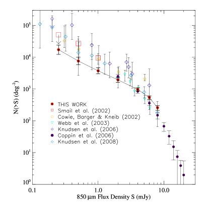
Figure 2.— Cumulative source counts $N(>S)$ derived from the Zemcov et al. (2007) catalog using the analysis described in the text (red points). The error bars account for the uncertainties associated with source flux measurement errors, gravitational lensing model uncertainties, flux boosting and cosmic variance. The other points are from the following sources: Smail et al. (2002), Cowie et al. (2002), Webb et al. (2003), Knudsen et al. (2006), Coppin et al. (2006), and Knudsen et al. (2008).

Table 2$N(>S)$ Measurements from this Work.

$S$ (mJy)	$N(>S)$ (deg-2)	$\sigma_{N+}$ (deg-2)	$\sigma_{N-}$ (deg-2)
8	259	41	45
6	541	68	74
4	974	119	109
2	1950	340	310
1	3730	950	720
0.5	7620	2410	1810
0.25	17300	6700	5000

Our catalog surveys a larger set of clusters than any previous work, with a factor of $\sim 2$ more area at the source plane, and thus produces statistically tighter error bars. Importantly, the sources in this catalog are sampled from clusters which were not necessarily selected for their strong gravitational lensing. We believe our data are less biased than some previous lensing surveys. Several of the targets – Abell 2218 and MS$0451.6{-}0305$ are examples – are known to contain strongly lensed sources. Previous work is concentrated on these and similar fields to yield the largest number of sources per cluster with a median number of sources per cluster field of $4$. In contrast, the catalog used here has a median number of two sources per cluster field. Another difference from previous work is the conservative data analysis and point-source extraction used in Zemcov et al. (2007) which led to the catalog used here. In that work, it was found that many sources from previous analyses drop significantly below the selection threshold.

To check whether systematic artifacts dominate the difference between this work and prior number counts, we have divided our catalog in several ways: into subsamples based on catalogs presented in previous work (that of Smail et al. 2002 and Cowie et al. 2002), into targets with integration times longer and shorter than $15\,$ks; and the analysis is repeated on these subsets. We find that the subsamples are consistent with the results presented for our full catalog and are lower than those from previous work. This is evidence that the subset of very deep or previously studied clusters have little statistical difference from the overall set.

Figure 3.— Comparison of counts measured near $850\,\mu$m and model predictions. The diamonds show the points measured in this work, the triangles are the counts measured by SHADES (Coppin et al., 2006) and the dots are the counts measured by LESS (Weiß et al., 2009) where the source flux axis has been scaled by a factor $(870\,\mu\mathrm{m}/850\,\mu\mathrm{m})^{3.5}$, (amounting to a few percent) to account for the difference in the centroid wavelengths of SCUBA and LABOCA. The solid line shows the best fit of Equation (1) as described in the text. The dashed line shows the prediction using the model of Lagache et al. (2003), and the dot-dashed line shows the prediction for the model of Valiante et al. (2009). Both models require a break at $\sim 1\,$mJy to obtain a total CIB consistent with the FIRAS result. The break in counts at $\approx 8$mJy hinted in the LESS and SHADES work and presented here shows that the unverified second break in the counts at $1\,$mJy is not required to match the total CIB intensity.

The $850\,\mu$m counts found here are plotted in Figure 3 along with the most precise measurements at brighter fluxes from SHADES (Coppin et al., 2006) using SCUBA and LESS using the LABOCA instrument at $870\,\mu$m (Weiß et al., 2009). Model predictions from Lagache et al. (2003) and Valiante et al. (2009) are also shown. The shapes of the SCUBA and LABOCA points are very similar, though the LESS source density is a bit lower. The bright end of the lensed counts presented here are higher than either of the direct surveys, and we believe that our brightest few points may be biased high due to misidentification of a handful of cluster member sources as weakly lensed objects. Our survey is an unbiased count of lensed objects since clusters are not expected to be particularly aligned with background sources, but clearly the number density of cluster members is a biased estimator of the general isotropic source density. Incorrectly counting cluster members as unit-magnification background galaxies would inflate the brightest counts above the pure background-only count locus.

The data support a single break in a power-law distribution, as in Equation (1), with the break occurring at $S_{0}=7$ or 8 mJy. At the same time, it is clear that the full data sets are not consistent with each other given the quoted uncertainties. In fitting Equation (1) to the data, we hold $\beta$ fixed at 5.1, taken from Coppin et al., choose $S_{0}$ and then fit $N_{0}$ and $\alpha$ to our five lowest flux data points. In this procedure, the choice of $S_{0}$ essentially sets the level of the brightest counts with $8\,$mJy running through the SHADES points and $\approx 7\,$mJy matching LESS. Reasonable choices of $S_{0}$ have approximately a 1% effect on the inferred total flux of $850\,\mu$m sources. Our best fit for $S_{0}=8\,$mJy is shown as a solid line in Figure 3.

The total brightness of the sky contributed by all sources brighter than $S_{1}$ is

$$I(\nu)=\int_{S_{1}}^{\infty}S\frac{dN}{dS}dS=\\ N_{0}S_{0}^{2}\left[\frac{1}{\beta-2}+\frac{1-(S_{1}/S_{0})^{2-\alpha}}{2-\alpha}\right]$$ (4)

(where $\alpha=2$ would be treated as a special case). Values of $\nu I(\nu)$ corresponding to our best-fit value of $\alpha=1.86$ and to the $1\sigma$ error limits on $\alpha$ are listed in Table 3 in units of nW m^-2 sr^-1 for several choices of the lower limit in flux, $S_{1}$. A summary is plotted in Figure 4. The firas experiment on cobe (Mather et al., 1994) measured the total extragalactic background in the SCUBA band to be in the range $3-5\times 10^{-10}\,$W m^-2 sr^-1 (Fixsen et al. 1998; Puget et al. 1996). Given that only approximately half the total intensity of the CIB at $850\,\mu$m comes from sources with $S\geq 100\,\mu$Jy accessible to SCUBA lensing surveys, our constraints on the total brightness of the CIB from sources do not add to the precision available from FIRAS for the total intensity of the CIB. At the same time, it is clear that the data do not require any break in the observed low-flux power law in order to be consistent with the FIRAS limits. Previous source number count determinations using SCUBA have the property that the extrapolation of $N(>S)$ over all fluxes overproduces this total CIB by a significant amount; in order to avoid this problem, either a second sharp break or a shallower faint count index would have been needed.

Table 3CIB Fluxes Varying $\alpha$.

$\alpha$	$N_{o}$	$\nu I$ all $S$	$S\geq 10\mu$Jy	$S\geq 100\mu$Jy	$S\geq 250\mu$Jy
	(deg-2 mJy-1)	(nW m-2 sr-1)	(nW m-2 sr-1)	(nW m-2 sr-1)	(nW m-2 sr-1)
1.78	98.0	0.340	0.269	0.221	0.194
1.86	92.0	0.494	0.309	0.238	0.203
1.92	86.8	0.848	0.364	0.266	0.222

Predictions given by the models of the infrared background source population shown in Figure 3 qualitatively reproduce the observed source density, steep slope, and break in the power law. However, they exhibit a break at $\sim 1\,$mJy which follows from matching the evolution of the sources to the counts throughout the infrared regime. Altering simply the luminosity evolution terms in these models could match the faint counts but would not move the break in the power law to match the data. More thorough exploration of the combined effects of the luminosity and density evolution to understand disagreement between models and observations should be addressed in future work.

In addition to the counts determined here at $850\,\mu$m, source counts from the BLAST instrument working at shorter sub-mm wavelengths also show a flattening of the faint end of the curve (Patanchon et al., 2009). Furthermore, deep observations of a lensing cluster with LABOCA independently suggest that the $S_{870\,\mu\mathrm{m}}<2\,$mJy part of the $N(>S)$ curve has a flatter slope than previously measured (Johansson et al., 2010). These results corroborate our suggestion that the slope of the faint end of the sub-mm source counts has been overestimated.

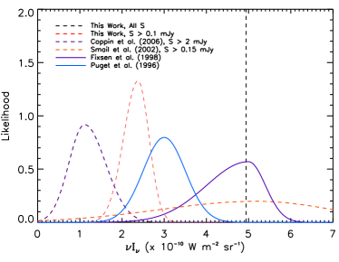
Figure 4.— Likelihoods of selected measurements of the extragalactic background at $850\,\mu$m; those measured by integrating various estimates of the FIRAS extragalactic background spectrum over the SCUBA band are shown as solid lines, while lower limits on the CIB from integrating the SCUBA source counts are shown as dashed. The red dashed line shows the limit on the CIB resulting when the counts presented here are integrated to $S\geq 0.10\,$mJy; the PDF has a width which is the quadrature sum of the uncertainties on the best fitting $\alpha$ and $N_{0}$ described in the text. The dashed black line shows the limits which result when the best-fitting $N(>S)$ model is extrapolated to $S=0\,$mJy. The measurement of Coppin et al. (2006), which integrates the number counts to $S\geq 2\,$mJy, and a representative result from earlier SCUBA surveys of lensing clusters integrating the counts down to $S\geq 0.15\,$mJy are shown; because their power laws are steeper, these yield much larger intensities if their best-fit models are extrapolated to very faint flux.

The key to future measurements attempting to resolve the $850\,\mu$m background into individual sources will be to survey large numbers of galaxy clusters to find rare, highly magnified images of very dim sources. Experiments such as SCUBA-2 (Holland et al., 2006) will allow mapping of $>100$ cluster fields to the confusion limit of the JCMT in a matter of weeks of observing time. This can be compared to the performance expected from ALMA, which will have much better angular resolution than any single-dish instrument but a very small field of view. At $350\,$GHz, ALMA can generate a mosaicked map of the central $r=2^{\prime}$ of a cluster in about 100 pointings, each requiring $\sim 3$ minutes to complete. In contrast, SCUBA-2 can make confusion noise dominated maps of clusters far beyond this central region with an instrument noise of $0.5\,$mJy in $\sim 1$ hr. Per cluster, this is a raw mapping speed advantage of a factor of 5 over ALMA on the central area; a survey strategy which would be maximally efficient would be to find bright sources with SCUBA-2 and follow up the central regions near the caustic lines with ALMA when interesting sources have been identified.

Should a survey from a bolometric camera find bright sources in many clusters, it will be difficult to apply very detailed lens models to all of them, particularly ones found in upcoming millimeter SZ effect surveys which may not have ancillary data on which to rely. Statistical approaches like or more mature than the one adopted in this work will be useful for analyzing those data. More effort to create high fidelity lensing models – even if only accurate on average – based on simple observable quantities is certainly justified.

That said, precise mass models of individual clusters which reduce the uncertainties on the source plane properties of highly magnified sources remain a very important component of these studies. Simple models are not very accurate when studying individual sources, so it is certainly worth expending the time and effort required to generate detailed lensing models. Combined with such models, the data produced by very high angular resolution instruments like ALMA will surely allow us the best view of the faintest galaxies making up the sub-mm background.

References

- Aretxaga et al. (2007) Aretxaga, I., et al. 2007, MNRAS, 379, 1571
- Barger et al. (1999) Barger, A. J., Cowie, L. L., & Sanders, D. B. 1999, ApJL, 518, L5
- Barger et al. (1998) Barger, A. J., Cowie, L. L., Sanders, D. B., Fulton, E., Taniguchi, Y., Sato, Y., Kawara, K., & Okuda, H. 1998, Nature, 394, 248
- Blain (1997) Blain, A. W. 1997, MNRAS, 290, 553
- Blain et al. (1999) Blain, A. W., Kneib, J.-P., Ivison, R. J., & Smail, I. 1999, ApJL, 512, L87
- Borgani et al. (1999) Borgani, S., Girardi, M., Carlberg, R. G., Yee, H. K. C., & Ellingson, E. 1999, ApJ, 527, 561
- Borys et al. (2003) Borys, C., Chapman, S., Halpern, M., & Scott, D. 2003, MNRAS, 344, 385
- Chapman et al. (2002) Chapman, S. C., Scott, D., Borys, C., & Fahlman, G. G. 2002, MNRAS, 330, 92
- Coppin et al. (2006) Coppin, K., et al. 2006, MNRAS, 372, 1621
- Cowie et al. (2002) Cowie, L. L., Barger, A. J., & Kneib, J.-P. 2002, AJ, 123, 2197
- Crawford et al. (2006) Crawford, S. M., Bershady, M. A., Glenn, A. D., & Hoessel, J. G. 2006, ApJL, 636, L13
- Cypriano et al. (2005) Cypriano, E. S., Lima Neto, G. B., Sodré, Jr., L., Kneib, J.-P., & Campusano, L. E. 2005, ApJ, 630, 38
- Cypriano et al. (2004) Cypriano, E. S., Sodré, L. J., Kneib, J.-P., & Campusano, L. E. 2004, ApJ, 613, 95
- Eales et al. (2000) Eales, S., Lilly, S., Webb, T., Dunne, L., Gear, W., Clements, D., & Yun, M. 2000, AJ, 120, 2244
- Elíasdóttir et al. (2007) Elíasdóttir, Á., et al. 2007, arXiv:0710.5636
- Fadda et al. (1996) Fadda, D., Girardi, M., Giuricin, G., Mardirossian, F., & Mezzetti, M. 1996, ApJ, 473, 670
- Fischer & Tyson (1997) Fischer, P., & Tyson, J. A. 1997, AJ, 114, 14
- Fixsen et al. (1998) Fixsen, D. J., Dwek, E., Mather, J. C., Bennett, C. L., & Shafer, R. A. 1998, ApJ, 508, 123
- Goto et al. (2003) Goto, T., Yamauchi, C., Fujita, Y., Okamura, S., Sekiguchi, M., Smail, I., Bernardi, M., & Gomez, P. L. 2003, MNRAS, 346, 601
- Holland et al. (2006) Holland, W., et al. 2006, in Presented at the Society of Photo-Optical Instrumentation Engineers (SPIE) Conference, Vol. 6275, Millimeter and Submillimeter Detectors and Instrumentation for Astronomy III. Edited by Zmuidzinas, Jonas; Holland, Wayne S.; Withington, Stafford; Duncan, William D.. Proceedings of the SPIE, Volume 6275, pp. 62751E (2006).
- Holland et al. (1999) Holland, W. S., et al. 1999, MNRAS, 303, 659
- Hughes et al. (1998) Hughes, D. H., et al. 1998, Nature, 394, 241
- Johansson et al. (2010) Johansson, D., et al. 2010, A&A, 514, A77+
- Jullo et al. (2007) Jullo, E., Kneib, J., Limousin, M., Elíasdóttir, Á., Marshall, P. J., & Verdugo, T. 2007, New Journal of Physics, 9, 447
- Knudsen et al. (2006) Knudsen, K. K., et al. 2006, MNRAS, 368, 487
- Knudsen et al. (2008) Knudsen, K. K., van der Werf, P. P., & Kneib, J.-P. 2008, MNRAS, 384, 1611
- Lagache et al. (2003) Lagache, G., Dole, H., & Puget, J. 2003, MNRAS, 338, 555
- Lagache et al. (2005) Lagache, G., Puget, J.-L., & Dole, H. 2005, Ann. Rev. Astron˙& Astrophys., 43, 727
- Li & Ostriker (2002) Li, L.-X., & Ostriker, J. P. 2002, ApJ, 566, 652
- Limousin et al. (2007) Limousin, M., et al. 2007, ApJ, 668, 643
- Łokas et al. (2006) Łokas, E. L., Prada, F., Wojtak, R., Moles, M., & Gottlöber, S. 2006, MNRAS, 366, L26
- Lubin et al. (1998) Lubin, L. M., Postman, M., & Oke, J. B. 1998, AJ, 116, 643
- Marsden et al. (2009) Marsden, G., et al. 2009, ApJ, 707, 1729
- Mather et al. (1994) Mather, J. C., et al. 1994, ApJ, 420, 439
- Mercurio et al. (2003) Mercurio, A., Girardi, M., Boschin, W., Merluzzi, P., & Busarello, G. 2003, A & A, 397, 431
- Natarajan & Springel (2004) Natarajan, P., & Springel, V. 2004, ApJL, 617, L13
- Navarro et al. (1996) Navarro, J. F., Frenk, C. S., & White, S. D. M. 1996, ApJ, 462, 563
- Negrello et al. (2007) Negrello, M., Perrotta, F., González-Nuevo, J., Silva, L., de Zotti, G., Granato, G. L., Baccigalupi, C., & Danese, L. 2007, MNRAS, 377, 1557
- Patanchon et al. (2009) Patanchon, G., et al. 2009, ApJ, 707, 1750
- Pimbblet et al. (2006) Pimbblet, K. A., Smail, I., Edge, A. C., O’Hely, E., Couch, W. J., & Zabludoff, A. I. 2006, MNRAS, 366, 645
- Poggianti et al. (2006) Poggianti, B. M., et al. 2006, ApJ, 642, 188
- Proust et al. (2000) Proust, D., Cuevas, H., Capelato, H. V., Sodré, Jr., L., Tomé Lehodey, B., Le Fèvre, O., & Mazure, A. 2000, A & A, 355, 443
- Puget et al. (1996) Puget, J.-L., Abergel, A., Bernard, J.-P., Boulanger, F., Burton, W. B., Desert, F.-X., & Hartmann, D. 1996, A & A, 308, L5+
- Rosati et al. (1999) Rosati, P., Stanford, S. A., Eisenhardt, P. R., Elston, R., Spinrad, H., Stern, D., & Dey, A. 1999, AJ, 118, 76
- Scott et al. (2002) Scott, S. E., et al. 2002, MNRAS, 331, 817
- Smail et al. (1997) Smail, I., Ivison, R. J., & Blain, A. W. 1997, ApJL, 490, L5+
- Smail et al. (2002) Smail, I., Ivison, R. J., Blain, A. W., & Kneib, J.-P. 2002, MNRAS, 331, 495
- Smith et al. (2005) Smith, G. P., Kneib, J.-P., Smail, I., Mazzotta, P., Ebeling, H., & Czoske, O. 2005, MNRAS, 359, 417
- Struble & Rood (1991) Struble, M. F., & Rood, H. J. 1991, ApJS, 77, 363
- Tran et al. (1999) Tran, K.-V. H., Kelson, D. D., van Dokkum, P., Franx, M., Illingworth, G. D., & Magee, D. 1999, ApJ, 522, 39
- Valiante et al. (2009) Valiante, E., Lutz, D., Sturm, E., Genzel, R., & Chapin, E. L. 2009, ApJ, 701, 1814
- Webb et al. (2003) Webb, T. M. A., Lilly, S. J., Clements, D. L., Eales, S., Yun, M., Brodwin, M., Dunne, L., & Gear, W. K. 2003, ApJ, 597, 680
- Weiß et al. (2009) Weiß, A., et al. 2009, ApJ, 707, 1201
- Wright & Brainerd (2000) Wright, C. O., & Brainerd, T. G. 2000, ApJ, 534, 34
- Wu et al. (1999) Wu, X.-P., Xue, Y.-J., & Fang, L.-Z. 1999, ApJ, 524, 22
- Zemcov et al. (2007) Zemcov, M., Borys, C., Halpern, M., Mauskopf, P., & Scott, D. 2007, MNRAS, 376, 1073