Uncovering the Riffled Independence Structure of Rankings
Abstract
Representing distributions over permutations can be a daunting task due to the fact that the number of permutations of objects scales factorially in . One recent way that has been used to reduce storage complexity has been to exploit probabilistic independence, but as we argue, full independence assumptions impose strong sparsity constraints on distributions and are unsuitable for modeling rankings. We identify a novel class of independence structures, called riffled independence, encompassing a more expressive family of distributions while retaining many of the properties necessary for performing efficient inference and reducing sample complexity. In riffled independence, one draws two permutations independently, then performs the riffle shuffle, common in card games, to combine the two permutations to form a single permutation. Within the context of ranking, riffled independence corresponds to ranking disjoint sets of objects independently, then interleaving those rankings. In this paper, we provide a formal introduction to riffled independence and present algorithms for using riffled independence within Fourier-theoretic frameworks which have been explored by a number of recent papers. Additionally, we propose an automated method for discovering sets of items which are riffle independent from a training set of rankings. We show that our clustering-like algorithms can be used to discover meaningful latent coalitions from real preference ranking datasets and to learn the structure of hierarchically decomposable models based on riffled independence.
keywords:
[class=AMS]keywords:
math.PR/0000000 \startlocaldefs \endlocaldefs
and
1 Introduction
Ranked data appears ubiquitously in various statistics and machine learning application domains. Rankings are useful, for example, in reasoning about preference lists in surveys [Kamishima, 2003], search results in information retrieval applications [M. Sun, 2010], and ballots in certain elections [Diaconis, 1989] and even the ordering of topics and paragraphs within a document [Chen et al., 2009]. The problem of building statistical models on rankings has thus been an important research topic in the learning community. As with many challenging learning problems, one must contend with an intractably large state space when dealing with rankings since there are ways to rank objects. In building a statistical model over rankings, simple (yet flexible) models are therefore preferable because they are typically more computationally tractable and less prone to overfitting.
A popular and highly successful approach for achieving such simplicity for distributions involving large collections of interdependent variables has been to exploit conditional independence structures (e.g., naive Bayes, tree, Markov models). With ranking problems, however, independence-based relations are typically trickier to exploit due to the so-called mutual exclusivity constraints which constrain any two items to map to different ranks in any given ranking.
In this paper, we present a novel, relaxed notion of independence, called riffled independence, in which one ranks disjoint subsets of items independently, then interleaves the subset rankings to form a joint ranking of the item set. For example, if one ranks a set of food items containing fruits and vegetables by preference, then one might first rank the vegetable and fruit sets separately, then interleave the two rankings to form a ranking for the full item set. Riffled independence appears naturally in many ranked datasets — as we show, political coalitions in elections which use the STV (single transferable vote) voting mechanism typically lead to pronounced riffled independence constraints in the vote histograms.
Chaining the interleaving operations recursively leads to a simple, interpretable class of models over rankings, not unlike graphical models. We present methods for learning the parameters of such models and for estimating their structure.
The following is an outline of our main contributions as well as a roadmap for the sections ahead.111 This paper is an extended presentation of our previous papers [Huang and Guestrin, 2009a], which was the first introduction of riffled independence, and [Huang and Guestrin, 2010], which studied hierarchical models based on riffle independent decompositions.
- •
-
•
In Section 3, we introduce our main contribution: an intuitive, novel generalization of the notion of independence for permutations, riffled independence, based on interleaving independent rankings of subsets of items. We show riffled independence to be a more appropriate notion of independence for ranked data and exhibit evidence that riffle independence relations can approximately hold in real ranked datasets. We also discuss ideas for exploiting riffled independence relations in a distribution to reduce sample complexity and to perform efficient inference.
-
•
Within the same section, we introduce a novel family of distributions over the set of interleavings of two item sets, called biased riffle shuffles, that are useful in the context of riffled independence. We propose an efficient recursive procedure for computing the Fourier transform of these biased riffle shuffle distributions,
-
•
In Section 5, we discuss the problem of estimating model parameters of a riffle independent model from ranking data, and computing various statistics from model parameters. To perform such computations in a scalable way, we develop algorithms that can be used in the Fourier-theoretic framework of Kondor, Howard and Jebara [2007], Huang et al. [2009], and Huang, Guestrin and Guibas [2009b] for joining riffle independent factors (RiffleJoin), and for teasing apart the riffle independent factors from a joint (RiffleSplit), and provide theoretical and empirical evidence that our algorithms perform well.
-
•
We use Section 6 to define a family of simple and interpretable, yet flexible distributions over rankings, called hierarchical riffle independent models, in which subsets of items are iteratively interleaved into larger and larger subsets in a recursive stagewise fashion.
-
•
Sections 7, 8, and 9 tackle the problem of structure learning for our riffle independent models. In Section 7, we propose a method for finding the partitioning of the item set such that the subsets of the partition are as close to riffle independent as possible. In particular, we propose a novel objective for quantifying the degree to which two subsets are riffle independent to each other. In Section 8 and 9 we apply our partitioning algorithm to perform model selection from training data in polynomial time, without having to exhaustively search over the exponentially large space of hierarchical structures.
-
•
Finally in Section 11, we apply our algorithms to a number of datasets both simulated and real in order to validate our methods and assumptions. We show that our methods are indeed effective, and apply them in particular to various voting and preference ranking datasets.
2 Distributions on rankings
In this paper, we will be concerned with distributions over rankings. A ranking is a one-to-one association between items and ranks, where means that the item is assigned rank under . By convention, we will think of low ranked items as being preferred over higher ranked items (thus, ranking an item in first place means that it is the most preferred out of all items). We will also refer to a ranking by its inverse, (called an ordering and denoted with double brackets instead of parentheses), where also means that the item is assigned rank under . The reason for using both notations is due to the fact that certain concepts will be more intuitive to express using either the ranking or ordering notation.
Example 1.
As a running example in this paper, we will consider ranking a small list of 6 items consisting of fruits and vegetables enumerated below:
The ranking means, for example, that Corn is ranked third, Peas is ranked first, Lemon is ranked fifth, and so on. In ordering notation, the same ranking is expressed as: . Finally we will use to denote the rank of the third item, Lemon.
Permutations and the symmetric group
Rankings are similar to permutations, which are 1-1 mappings from the set into itself, the subtle difference being that rankings map between two different sets of size . In this paper, we will use the same notation for permutations and rankings, but use permutations to refer to (1-1) functions which rearrange the ordering of the item set or the ranks. If is a permutation of the set of ranks, then then given a ranking , one can rearrange the ranks by left-composing with . Thus, the ranking maps item to rank . On the other hand, if is a permutation of the item set, one can rearrange the item set by right-composing with . Thus, if item was relabeled as item , then returns the rank of item with respect to the original item ordering. Finally, we note that the composition of any two permutations is itself a permutation, and the collection of all permutations forms a group, commonly known as the symmetric group, or .222We will sometimes abusively denote the set of rankings by . Strictly speaking, however, the rankings are not a group, and instead one says that acts faithfully on rankings.
A distribution , defined over the set of rankings or permutations can be viewed as a joint distribution over the variables (where ), subject to mutual exclusivity constraints which stipulate that two objects cannot simultaneously map to the same rank, or alternatively, that two ranks cannot simultaneously be occupied by the same object ( whenever ).
Example 2 (APA election data).
As a running example throughout the paper (in addition to the fruits and vegetables), we will analyze the well known APA election dataset that was first used by Diaconis [1988] and has since been analyzed in a number of ranking studies. The APA dataset is a collection of 5738 ballots from a 1980 presidential election of the American Psychological Association where members rank ordered five candidates from favorite to least favorite. The names of the five candidates that year were (1) William Bevan, (2) Ira Iscoe, (3) Charles Kiesler, (4) Max Siegle, and (5) Logan Wright [Marden, 1995].
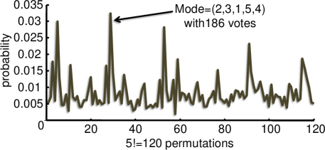
Since there are five candidates, there are possible rankings. In Figure 1 we plot the proportion of votes that each ranking received. Interestingly, instead of concentrating at just a small set of rankings, the vote distribution in the APA dataset is fairly diffuse with every ranking receiving some number of votes. The mode of the vote distribution occurs at the ranking with 186 votes.
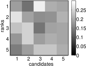
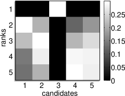
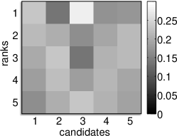
For interpretability, we also visualize the matrix of first-order marginals in which the entry represents the number of voters who assigned rank to candidate . Figure 1 represents the first-order matrix using grayscale levels to represent numbers of voters. What can be seen is that overall, candidate 3 (C. Kiesler) received the highest number of votes for rank 1 (and incidentally, won the election). The vote distribution gives us a story that goes far deeper than simply telling us who the winner was, however. Diaconis [1988], for example, noticed that candidate 3 also had a significant “hate” vote — a good number of voters placed him in the last rank. Throughout this paper, we will let this story unfold via a series of examples based on the APA dataset.
2.1 Dealing with factorial possibilities
The fact that there are factorially many possible rankings poses a number of significant challenges for learning and inference. First, there is no way to tractably represent arbitrary distributions over rankings for large . Storing an array of doubles, for example, requires roughly 14 gigabytes of storage, which is beyond the RAM capacity of a typical modern PC. Second, the naive algorithmic complexity of common probabilistic operations is also intractable for such distributions. Computing the marginal probability, , that item is preferred to item , for example, requires a summation over elements. Finally, even if storage and computation issues were resolved, one would still have sample complexity issues to contend with — for nontrivial , it is impractical to hope that each of the possible rankings would appear even once in a training set of rankings. The only existing datasets in which every possible ranking is realized are those for which , and in fact, the APA dataset (Example 2) is the only such dataset for that we are aware of.
The quest for exploitable problem structure has led researchers in machine learning and related fields to consider a number of possibilities including distribution sparsity [Reid, 1979; Jagabathula and Shah, 2008; Farias, Jagabathula and Shah, 2009], exponential family parameterizations [Meila et al., 2007; Helmbold and Warmuth, 2007; Lebanon and Mao, 2008; Petterson et al., 2009], algebraic/Fourier structure [Kondor, Howard and Jebara, 2007; Kondor and Borgwardt, 2008; Huang, Guestrin and Guibas, 2007, 2009b], and probabilistic independence [Huang et al., 2009]. We briefly summarize several of these approaches in the following.
Parametric models
We will not be able to do justice to the sheer volume of previous work on parametric ranking models. Parametric probabilistic models over the space of rankings have a rich tradition in statistics, [Thurstone, 1927; Mallows, 1957; Plackett, 1975; Marden, 1995; Fligner and Verducci, 1986, 1988; Meila et al., 2007; Guiver and Snelson, 2009], and to this day, researchers continue to expand upon this body of work. For example, the well known Mallows model (which we will discuss in more detail in Section 6), which is often thought of as an analogy of the normal distribution for permutations, parameterizes a distribution with a “mean” permutation and a precision/spread parameter.
The models proposed in this paper generalize some of the classical models from the statistical ranking literature, allowing for more expressive distributions to be captured. At the same time, our methods form a conceptual bridge to popular models (i.e., graphical models) used in machine learning which, rather than relying on a prespecified parametric form, simply work within a family of distributions that are consistent with some set of conditional independence assumptions [Koller and Friedman, 2009].
Sparse methods
Sparse methods for summarizing distributions range from older ad-hoc approaches such as maintaining -best hypotheses [Reid, 1979] to the more updated compressed sensing inspired approaches discussed in [Jagabathula and Shah, 2008; Farias, Jagabathula and Shah, 2009]. Such approaches assume that there are at most permutations which own all (or almost all) of the probability mass, where scales either sublinearly or as a low degree polynomial in . While sparse distributions have been successfully applied in certain tracking domains, we argue that they are often less suitable in ranking problems where it might be necessary to model indifference over a large subset of objects.333 In some situations, particularly when one is interested primarily in accurately capturing a loss or payoff function instead of raw ranking probabilities, it can suffice to use a sparse proxy distribution even if the true underlying distribution is not itself sparse. See, for example, [Helmbold and Warmuth, 2007; Farias, Jagabathula and Shah, 2009] for details. If one is approximately indifferent among a subset of objects, then there are at least rankings with nonzero probability mass. As an example, one can see that the APA vote distribution (Figure 1) is clearly not a sparse distribution, with each ranking having received some nonzero number of votes.
Fourier-based (low-order) methods
Another recent thread of research has centered around Fourier-based methods which maintain a set of low-order summary statistics [Shin et al., 2005; Diaconis, 1988; Kondor, 2008; Huang, Guestrin and Guibas, 2009b]. The first-order summary, for example, stores a marginal probability of the form for every pair and thus requires storing a matrix of only numbers. In our fruits/vegetables example, we might store the probability that Figs are ranked first, or the probability that Peas is ranked last.
Example 3 (APA election data (continued)).
In the following matrix, we record the first order matrix computed from the histogram of votes in the APA election example (also visualized using grayscale levels in Figure 1). Dividing each number by the total number of votes would yield a matrix of first order marginal probabilities.
More generally, one might store -order marginals, which are marginal probabilities of -tuples. The second-order marginals, for example, take the form , (perhaps encoding the joint probability that Grapes are ranked first, and Peas second) and require storage.
Low-order marginals turn out to be intimately related to a generalized form of Fourier analysis. Generalized Fourier transforms for functions on permutations have been studied for several decades now primarily by Persi Diaconis and his collaborators [Diaconis, 1988; Clausen and Baum, 1993; Maslen, 1998; Terras, 1999; Rockmore, 2000]. Low-order marginals correspond, in a certain sense, to the low-frequency Fourier coefficients of a distribution over permutations. For example, the first-order matrix of can be reconstructed exactly from of the lowest frequency Fourier coefficients of , and the second-order matrix from of the lowest frequency Fourier coefficients. From a Fourier theoretic perspective, one sees that low order marginals are not just a reasonable way of summarizing a distribution, but can actually be viewed as a principled “low frequency” approximation thereof. In contrast with sparse methods, Fourier-based methods handle diffuse distributions well but are not easily scalable without making aggressive independence assumptions [Huang et al., 2009] since, in general, one requires coefficients to exactly reconstruct -order marginals, which quickly becomes intractable for moderately large .
2.2 Fully independent subsets of items
To scale to larger problems, Huang et al. [2009] demonstrated that, by exploiting probabilistic independence, one could dramatically improve the scalability of Fourier-based methods, e.g., for tracking problems, since confusion in data association only occurs over small independent subgroups of objects in many problems. Probabilistic independence assumptions on the symmetric group can simply be stated as follows. Consider a distribution defined over . Let be a -subset of , say, and let be its complement () with size . We say that and are independent if
| (2.1) |
Storing the parameters for the above distribution requires keeping probabilities instead of the much larger size required for general distributions. Of course, can still be quite large. Typically, one decomposes the distribution recursively and stores factors exactly for small enough factors, or compresses factors using Fourier coefficients (but using higher frequency terms than what would be possible without the independence assumption). In order to exploit probabilistic independence in the Fourier domain, Huang et al. [2009] proposed algorithms for joining factors and splitting distributions into independent components in the Fourier domain.
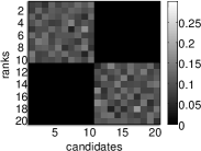
Despite its utility for many tracking problems, however, we argue that the independence assumption on permutations implies a rather restrictive constraint on distributions, rendering independence highly unrealistic in ranking applications. In particular, using the mutual exclusivity property, it can be shown [Huang et al., 2009] that, if and are independent, then and are not allowed to map to the same ranks. That is, for some fixed -subset , is a permutation of elements in and is a permutation of its complement, , with probability 1.
Example 4.
Continuing with our vegetable/fruit example with , if the vegetable and fruit rankings,
are known to be independent. Then for , the vegetables occupy the first and second ranks with probability one, and the fruits occupy ranks with probability one, reflecting that vegetables are always preferred over fruits according to this distribution.
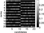
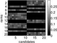
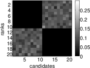
Huang et al. [2009] refer to this restrictive constraint as the first-order condition because of the block structure imposed upon first-order marginals (see Figure 2). In sports tracking, permutations represent the mapping between the identities of players with positions on the field, and in such settings, the first-order condition might say, quite reasonably, that there is potential identity confusion within tracks for the red team and within tracks for the blue team but no confusion between the two teams. In our ranking example however, the first-order condition forces the probability of any vegetable being in third place to be zero, even though both vegetables will, in general, have nonzero marginal probability of being in second place, which seems quite unrealistic.
Example 5 (APA election data (continued)).
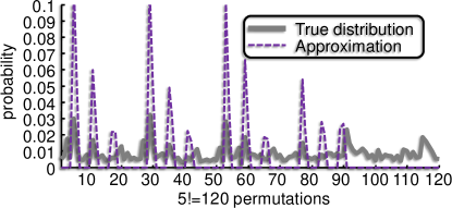
Consider approximating the APA vote distribution by a factorized distribution (as in Equation 2.1). In Figure 3, we plot (in solid purple) the factored distribution which is closest to the true distribution with respect to total variation distance. In our approximation, candidate 3 is constrained to be independent of the remaining four candidates and maps to rank 1 with probability 1.
While capturing the fact that the “winner” of the election should be candidate 3, the fully factored distribution can be seen to be a poor approximation, assigning zero probability to most permutations even if all permutations received a positive number of votes. Since the support of the true distribution is not contained within the support of the approximation, the KL divergence, is infinite.
In the next section, we overcome the restrictive first-order condition with the more flexible notion of riffled independence.
3 Riffled independence: definitions and examples
The riffle (or dovetail) shuffle [Bayer and Diaconis, 1992] is perhaps the most commonly used method of card shuffling, in which one cuts a deck of cards into two piles, and , with size and , respectively, and successively drops the cards, one by one, so that the two piles become interleaved (see Figure 4) into a single deck again. Inspired by the riffle shuffle, we present a novel relaxation of the full independence assumption, which we call riffled independence. Rankings that are riffle independent are formed by independently selecting rankings for two disjoint subsets of objects, then interleaving the two rankings using a riffle shuffle to form a final ranking over all objects. Intuitively, riffled independence models complex relationships within each set and while allowing correlations between the sets to be modeled only through a constrained form of shuffling.
Example 6.
Consider generating a ranking of vegetables and fruits. We might first ‘cut the deck’ into two piles, a pile of vegetables () and a pile of fruits (), and in a first stage, independently decide how to rank each pile. For example, within vegetables, we might decide that Peas are preferred to Corn: . Similarly, within fruits, we might decide on the following ranking: (Lemons preferred over Figs, Figs preferred over Grapes, Grapes preferred over Oranges).
In the second stage of our model, the fruit and vegetable rankings are interleaved to form a full preference ranking over all six items. For example, if the interleaving is given by: , then the resulting full ranking is:

3.1 Convolution based definition of riffled independence
There are two ways to define riffled independence, and, we will first provide a definition using convolutions, a view inspired by our card shuffling intuitions. Mathematically, shuffles are modeled as random walks on the symmetric group. The ranking after a shuffle is generated from the ranking prior to that shuffle, , by drawing a permutation, from an interleaving distribution , and setting (the composition of the mapping with ). Given the distribution over , we can find the distribution after the shuffle via the formula: . This operation which combines the distributions and is commonly known as convolution:
Definition 7.
Let and be probability distributions on . The convolution of the distributions is the function: We use the symbol to denote the convolution operation. Note that is not in general commutative (hence, ).
Besides the riffle shuffle, there are a number of different shuffling strategies — the pairwise shuffle, for example, simply selects two cards at random and swaps them. The question then, is what are interleaving shuffling distributions that correspond to riffle shuffles? To answer this question, we use the distinguishing property of the riffle shuffle, that, after cutting the deck into two piles of size and , it must preserve the relative ranking relations within each pile. Thus, if the card appears above the card in one of the piles, then after shuffling, the card remains above the card. In our example, relative rank preservation says that if Peas is preferred over Corn prior to shuffling, they continue to be preferred over Corn after shuffling. Any allowable riffle shuffling distribution must therefore assign zero probability to permutations which do not preserve relative ranking relations. As it turns out, the set of permutations which do preserve these relations have a simple description.
Definition 8 (Interleaving distributions).
The -interleavings are defined as the following set:
A distribution on is called an interleaving distribution if it assigns nonzero probability only to elements in .
The -interleavings can be shown to preserve relative ranking relations within each of the subsets and upon multiplication:
Lemma 9.
Let (or ) and let be any -interleaving in . Then if and only if (i.e., permutations in preserve relative ranking relations).
Example 10.
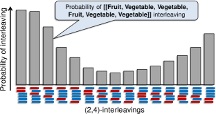
In our vegetable/fruits example, In our vegetable/fruits example, we have , (two vegetables, four fruits). The set of -interleavings is:
or written in ordering notation,
Note that the number of possible interleavings is . One possible riffle shuffling distribution on might, for example, assign uniform probability () to each permutation in and zero probability to everything else, reflecting indifference between vegetables and fruits. Figure 4 is a graphical example of a -interleaving distribution.
We now formally define our generalization of independence where a distribution which fully factors independently is allowed to undergo a single riffle shuffle.
Definition 11 (Riffled independence).
The subsets and are said to be riffle independent if , with respect to some interleaving distribution and distributions , respectively. We will notate the riffled independence relation as , and refer to as relative ranking factors.
Notice that without the additional convolution, the definition of riffled independence reduces to the fully independent case given by Equation 2.1.
Example 12.
Consider drawing a ranking from a riffle independent model. One starts with two piles of cards, and , stacked together in a deck. In our fruits/vegetables setting, if we always prefer vegetables to fruits, then the vegetables occupy positions and the fruits occupy positions . In the first step, rankings of each pile are drawn independent. For example, we might have the rankings: and , constituting a draw from the fully independent model described in Section 2.2. In the second stage, the deck of cards is cut and interleaved by an independently selected element . For example, if:
then the joint ranking is:
3.2 Alternative definition of riffled independence
It is possible to rewrite the definition of riffled independence so that it does not involve a convolution. We first define functions which map a given full ranking to relative rankings and interleavings for and .
Definition 13.
-
•
(Absolute ranks): Given a ranking , and a subset , denotes the absolute ranks of items in .
-
•
(Relative ranking map): Let denote the ranks of items in relative to the set . For example, in the ranking , the relative ranks of the vegetables is . Thus, while corn is ranked fifth in , it is ranked second in . Similarly, the relative ranks of the fruits is .
-
•
(Interleaving map): Likewise, let denote the way in which the sets and are interleaved by . For example, using the same as above, the interleaving of vegetables and fruits is . In ranking notation (as opposed to ordering notation), can be written as . Note that for every possible interleaving, there are exactly distinct permutations which are associated to by the interleaving map.
Using the above maps, the following lemma provides an algebraic expression for how any permutation can be uniquely decomposed into an interleaving composed with relative rankings of and , which have been “stacked” into one deck.
Lemma 14.
Let , and . Any ranking can be decomposed uniquely as an interleaving composed with a ranking of the form , where , , and means that the number is added to every rank in . Specifically, with , , and (Proof in Appendix).
Lemma 14 shows that one can think of a triplet as being coordinates which uniquely specify any ranking of items in . Using the decomposition, we can now state a second, perhaps more intuitive, definition of riffled independence in terms of the relative ranking and interleaving maps.
Definition 15.
Sets and are said to be riffle independent if and only if, for every , the joint distribution factors as:
| (3.1) |
Proof.
Assume that and are riffle independent with respect to Definition 11. We will show that Definition 15 is also satisfied (the opposite direction will be similar). Therefore, we assume that . Note that is supported on the subgroup .
Let be any ranking. We will need to use a simple claim: consider the ranking (where ). Then is an element of the subgroup if and only if .
Thus, we have shown that Definition 15 has been satisfied as well. ∎
Discussion
We have presented two ways of thinking about riffled independence. Our first formulation, in terms of convolution, is motivated by the connections between riffled independence and card shuffling theory. As we show in Section 5, the convolution based view is also crucial for working with Fourier coefficients of riffle independent distributions and analyzing the theoretical properties of riffled independence. Our second formulation on the other hand, shows the concept of riffled independence to be remarkably simple — that the probability of a single ranking can be computed without summing over all rankings (required in convolution) — a fact which may not have been obvious from Definition 11.
Finally, for interested readers, the concept of riffled independence also has a simple and natural group theoretic description. By a fully factorized distribution, we refer to a distribution supported on the subgroup , which factors along the and “dimensions”. As we have discussed, such sparse distributions are not appropriate for ranking applications, and one would like to work with distributions capable of placing nonzero probability mass on all rankings. In the case of the symmetric group, however, there is a third “missing dimension” — the coset space, . Thus, the natural extension of full independence is to randomize over a set of coset representatives of , what we have referred to in the above discussion as interleavings. The draws from each set, , , and are then independent in the ordinary sense, and we say that the item sets and are riffle independent.
Special cases
There are a number of special case distributions captured by the riffled independence model that are useful for honing intuition. We discuss these extreme cases in the following list.
-
•
(Uniform and delta distributions): Setting the interleaving distribution and both relative ranking factors to be uniform distributions yields the uniform distribution over all full rankings. Similarly, setting the same distributions to be delta distributions (which assign zero probability to all rankings but one) always yields a delta distribution.
It is interesting to note that while and are always fully independent under a delta distribution, they are never independent under a uniform distribution. However, both uniform and delta distributions factor riffle independently with respect to any partitioning of the item set. Thus, not only is riffle independent , but in fact, any set is riffle independent of its complement.
-
•
(Uniform interleaving distributions): Setting the interleaving distribution to be uniform, as we will discuss more in detail later, reflects complete indifference between the sets and , even if and encode complex preferences within each set alone.
-
•
(Uniform relative ranking factors): Setting the relative ranking factors, and to be uniform distributions means that with respect to the joint distribution , all items in are completely interchangeable amongst each other (as are all items in ).
-
•
(Delta interleaving distributions): Setting the interleaving distribution, , to be a delta distribution on any of the -interleavings in recovers the definition of ordinary probabilistic independence, and thus riffled independence is a strict generalization thereof (see Figure 2). Just as in the full independence regime, where the distributions and are marginal distributions of absolute rankings of and , in the riffled independence regime, and can be thought of as marginal distributions of the relative rankings of item sets and .
-
•
(Delta relative ranking factor): On the other hand, if one of the relative ranking factors, say , is a delta distribution and the other two distributions and are uniform, then the resulting riffle independent distribution can be thought of as an indicator function for the set of rankings that are consistent with one particular incomplete ranking (in which only the relative ranking of has been specified). Such distributions can be useful in practice when the input data comes in the form of incomplete rankings rather than full rankings.
Example 17 (APA election data (continued)).
Like the independence assumptions commonly used in naive Bayes models, we would rarely expect riffled independence to exactly hold in real data. Instead, it is more appropriate to view riffled independence assumptions as a form of model bias that ensures learnability for small sample sizes, which as we have indicated, is almost always the case for distributions over rankings.
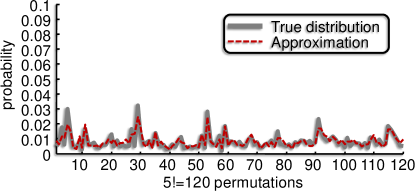
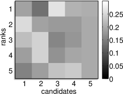
Can we ever expect riffled independence to be manifested in a real dataset? In Figure 5, we plot (in dotted red) a riffle independent approximation to the true APA vote distribution (in thick gray) which is optimal with respect to KL-divergence (we will explain how to obtain the approximation in the remainder of the paper). The approximation in Figure 5 is obtained by assuming that the candidate set is riffle independent of , and as can be seen, is quite accurate compared to the truth (with the KL-divergence from the true to the factored distribution being ). Figure 5 exhibits the first order marginals of the approximating distribution, which can also visually be seen to be a faithful approximation (see Figure 1). We will discuss the interpretation of the result further in Section 6.
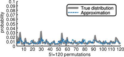
For comparison, we also display (in Figures 5 and 5) the result of approximating the true distribution by one in which candidate , the winner, is riffle independent of the remaining candidate. The resulting approximation is inferior, and the lesson to be learned in the example is that finding the correct/optimal partitioning of the item set is important in practice. We remark however, that the approximation obtained by factoring out candidate 3 is not a terrible approximation (especially on examining first order marginals), and that both approximations are far more accurate than the fully independent approximation showed earlier in Figure 3. The KL divergence from the true distribution to the factored distribution (with candidate 3 riffle independent of the remaining candidates) is .
3.3 Interleaving distributions
There is, in the general case, a significant increase in storage required for riffled independence over full independence. In addition to the storage required for distributions and , we now require storage for the nonzero terms of the riffle shuffling distribution . We now introduce a family of useful riffle shuffling distributions which can be described using only a handful of parameters. The simplest riffle shuffling distribution is the uniform riffle shuffle, , which assigns uniform probability to all -interleavings and zero probability to all other elements in . Used in the context of riffled independence, models potentially complex relations within and , but only captures the simplest possible correlations across subsets. We might, for example, have complex preference relations amongst vegetables and amongst fruits, but be completely indifferent with respect to the subsets, vegetables and fruits, as a whole.
There is a simple recursive method for uniformly drawing -interleavings. Starting with a deck of cards cut into a left pile () and a right pile (), pick one of the piles with probability proportional to its size ( for the left pile, for the right) and drop the bottommost card, thus mapping either card or card to rank . Then recurse on the remaining undropped cards, drawing a -interleaving if the right pile was picked, or a -interleaving if the left pile was picked. See Algorithm 1.
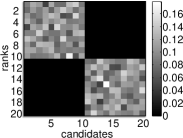
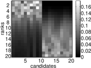
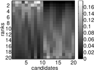
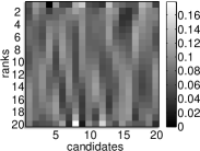
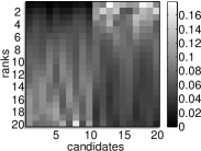
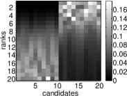
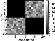
It is natural to consider generalizations where one is preferentially biased towards dropping cards from the left hand over the right hand (or vice-versa). We model this bias using a simple one-parameter family of distributions in which cards from the left and right piles drop with probability proportional to and , respectively, instead of and . We will refer to as the bias parameter, and the family of distributions parameterized by as the biased riffle shuffles.444The recurrence in Alg. 1 has appeared in various forms in literature [Bayer and Diaconis, 1992]. We are the first to (1) use the recurrence to Fourier transform , and to (2) consider biased versions. The biased riffle shuffles in Fulman [1998] are not similar to our biased riffle shuffles.
In the context of rankings, biased riffle shuffles provide a simple model for expressing groupwise preferences (or indifference) for an entire subset over or vice-versa. The bias parameter can be thought of as a knob controlling the preference for one subset over the other, and might reflect, for example, a preference for fruits over vegetables, or perhaps indifference between the two subsets. Setting or recovers the full independence assumption, preferring objects in (vegetables) over objects in (fruits) with probability one (or vice-versa), and setting , recovers the uniform riffle shuffle (see Fig. 6). Finally, there are a number of straightforward generalizations of the biased riffle shuffle that one can use to realize richer distributions. For example, might depend on the number of cards that have been dropped from each pile (allowing perhaps, for distributions to prefer crunchy fruits over crunchy vegetables, but soft vegetables over soft fruits).
4 Exploiting structure for probabilistic inference
In this section, we discuss a number of basic properties of riffled independence, which show that certain probabilistic inference operations can be accomplished by operating on a single factor rather than the entire joint distribution.
Upon knowing that is riffle independent of , an immediate consequence is that we can show, just as in the full independence regime, that conditioning operations on certain observations and MAP (maximum a posteriori) assignment problems decompose according to riffled independence structure. All of the following properties are straightforward to derive using the factorization in Definition 15.
Proposition 18 (Probabilistic inference decompositions).
-
•
(Conditioning): Consider prior and likelihood functions, and , on in which subsets and are riffle independent, with parameters and , respectively. Let denote the pointwise product operation between two functions. Then and are also riffle independent with respect to the posterior distribution under Bayes rule, which has interleaving distribution with relative ranking factors and , for and respectively.
-
•
(MAP assignment): Let and be riffle independent subsets. Consider the following permutations:
Then the mode of is composed with (i.e., ).
-
•
(Entropy): Consider riffle independent subsets and . The entropy of the joint distribution is given by: .
Some ranked datasets come in the form of pairwise comparisons, with records of the form “object is preferred to object ”. As a corollary to Proposition 18, we now argue that conditioning on these pairwise ranking likelihood functions (that depend only on whether object is preferred to object ) decomposes along riffled independence structures. The pairwise ranking model [Huang, Guestrin and Guibas, 2009b] for objects and , is defined over as:
and reflects the fact that object is preferred to object (with probability ). If objects and both belong to one of the sets, say , then only one factor requires an update using Bayes rule. If vegetables and fruits are riffle independent, for example, then less computation would be required to compare a vegetable against a vegetable than to compare a fruit against a vegetable. For example, the observation that Corn is preferred over Peas affects only the distribution, , over vegetables. More formally, we state this intuitive corollary as follows:
Corollary 19.
Consider conditioning on the pairwise ranking model, , and suppose that and are riffle independent subsets with respect to the prior distribution , with parameters , , . If , then and are riffle independent with respect to the posterior distribution, whose parameters are identical to those of the prior, except for the relative ranking factor corresponding to , which is .
Proof sketch.
First show that the subsets and are riffle independent with respect to the likelihood function, by equating the likelihood function to a product of a uniform interleaving distribution, , and relative ranking factor for , and a uniform relative ranking factor for . Then apply Proposition 18. ∎
Let us compare the result of the corollary to what is possible with a fully factored distribution. If and were fully independent, then conditioning on any distribution which involved items in (or only in ) would require only updating the factor associated with item set . For example, if , then first-order observations of the form “item is in rank ” can be efficiently conditioned in the fully independent scenario. With riffled independence, it is not, in general, possible to condition on such first-order observations without modifying all of the parameters. However, as Corollary 19 shows, pairwise comparisons involving both in (or both in ) can be performed exactly by updating either (or ) without having to touch all probabilities.
5 Algorithms for a fixed partitioning of the item set
We have thus far covered a number of intuitive examples and properties of riffled independence. Given a set of rankings drawn from some distribution , we are now interested in estimating a number of statistical quantities, such as the parameters of a riffle independent model. In this section, we will assume a known structure (that the partitioning of the item set into subsets and is known), and given such a partitioning of the item set, we are interested in the problem of estimating parameters (which we will refer to as RiffleSplit), and the inverse problem of computing probabilities (or marginal probabilities) with given parameters (which we will refer to as RiffleJoin).
RiffleSplit
In RiffleSplit (which we will also refer to as the parameter estimation problem), we would like to estimate various statistics of the relative ranking and interleaving distributions of a riffle independent distribution (, , and ). Given a set of i.i.d. training examples, , we might, for example, want to estimate each raw probability (e.g., estimate for each interleaving ). In general, we may be interested in estimating more general statistics (e.g., what are the second order relative ranking probabilities of the set of fruits?).
Since our variables are discrete, computing the maximum likelihood parameter estimates consists of forming counts of the number of training examples consistent with a given interleaving or relative ranking. Thus, the MLE parameters in our problem are simply given by the following formulas:
| (5.1) | ||||
| (5.2) | ||||
| (5.3) |
RiffleJoin
Having estimated parameters of a riffle independent distribution, we would like to now compute various statistics of the data itself. In the simplest case, we are interested in estimating , the joint probability of a single ranking, which can be evaluated simply by plugging parameter estimates of , , and into our second definition of riffled independence (Definition 15).
More generally however, we may be interested in knowing the low-order statistics of the data (e.g., the first order marginals, second order marginals, etc.), or related statistics (such as , the probability that object is preferred to object ). And typically for such low-order statistics, one must compute a sum over rankings. For example, to compute the probability that item is ranked in position , one must sum over rankings:
| (5.4) |
While Equation 5.4 may be feasible for small (such as on the APA dataset), the sum quickly grows to be intractable for larger . One of the main observations of the remainder of this section, however, is that low-order marginal probabilities of the joint distribution can always be computed directly from low-order marginal probabilities of the relative ranking and interleaving distributions without explicitly computing intractable sums.
5.1 Fourier theoretic algorithms for riffled independence
We now present algorithms for working with riffled independence (solving the RiffleSplit and RiffleJoin problems) in the Fourier theoretic framework of Kondor, Howard and Jebara [2007]; Huang et al. [2009]; Huang, Guestrin and Guibas [2009b]. The Fourier theoretic perspective of riffled independence presented here is valuable because it will allow us to work directly with low-order statistics instead of having to form the necessary raw probabilities first. Note that readers who are primarily interested in the structure learning can jump directly to Section 6.
We begin with a brief introduction to Fourier theoretic inference on permutations (see Kondor [2008]; Huang, Guestrin and Guibas [2009b] for a detailed exposition). Unlike its analog on the real line, the Fourier transform of a function on takes the form of a collection of Fourier coefficient matrices ordered with respect to frequency. Discussing the analog of frequency for functions on , is beyond the scope of our paper, and, given a distribution , we simply index the Fourier coefficient matrices of as , , , ordered with respect to some measure of increasing complexity. We use to denote the complete collection of Fourier coefficient matrices. One rough way to understand this complexity, as mentioned in Section 2, is by the fact that the low-frequency Fourier coefficient matrices of a distribution can be used to reconstruct low-order marginals. For example, the first-order matrix of marginals of can always be reconstructed from the matrices and . As on the real line, many of the familiar properties of the Fourier transform continue to hold. The following are several basic properties used in this paper:
Proposition 20 (Properties of the Fourier transform, Diaconis [1988]).
Consider any .
-
•
(Linearity) For any , holds at all frequency levels .
-
•
(Convolution) The Fourier transform of a convolution is a product of Fourier transforms: , for each frequency level , where the operation is matrix multiplication.
-
•
(Normalization) The first coefficient matrix, , is a scalar and equals .
A number of papers in recent years (Kondor, Howard and Jebara [2007]; Huang, Guestrin and Guibas [2007]; Huang et al. [2009]; Huang, Guestrin and Guibas [2009b]) have considered approximating distributions over permutations using a truncated (bandlimited) set of Fourier coefficients and have proposed inference algorithms that operate on these Fourier coefficient matrices. For example, one can perform generic marginalization, Markov chain prediction, and conditioning operations using only Fourier coefficients without ever having to perform an inverse Fourier transform.
In this section, we provide generalizations of the algorithms in Huang et al. [2009] that tackle the RiffleJoin and RiffleSplit problems. We will assume, without loss of generality that and (this assumption will be discarded in later sections), Although we begin each of the following discussions as if all of the Fourier coefficients are provided, we will be especially interested in algorithms that work well in cases where only a truncated set of Fourier coefficients are present, and where is only approximately riffle independent.
For both problems, we will rely on two Fourier domain algorithms introduced in Huang et al. [2009], Join and Split, as subroutines. Given independent factors and , Join returns the joint distribution . Conversely, given a distribution , Split computes and by marginalizing over or , respectively. For example, returns a function defined on , and . We will overload the Join/Split names to refer to both the ordinary and Fourier theoretic formulations of the same procedures.
5.2 RiffleJoin in the Fourier domain
Given the Fourier coefficients of , , and , we can compute the Fourier coefficients of using Definition 11 (our first definition) by applying the Join algorithm from Huang et al. [2009] and the Convolution Theorem (Proposition 20), which tells us that the Fourier transform of a convolution can be written as a pointwise product of Fourier transforms. To compute the , the Fourier theoretic formulation of the RiffleJoin algorithm simply calls the Join algorithm on and , and convolves the result by (see Algorithm 2).
In general, it may be intractable to Fourier transform the riffle shuffling distribution . However, there are some cases in which can be computed. For example, if is computed directly from a set of training examples, then one can simply compute the desired Fourier coefficients using the definition of the Fourier transform given in Huang, Guestrin and Guibas [2009b], which is tractable as long as the samples can be tractably stored in memory. For the class of biased riffle shuffles that we discussed in Section 3, one can also efficiently compute the low-frequency terms of by employing the recurrence relation in Algorithm 1. In particular, Algorithm 1 expresses a biased riffle shuffle on as a linear combination of biased riffle shuffles on . By invoking linearity of the Fourier transform (Proposition 20), one can efficiently compute via a dynamic programming approach quite reminiscent of Clausen’s FFT (Fast Fourier transform) algorithm Clausen and Baum [1993]. We describe our algorithm in more detail in Appendix B. To the best of our knowledge, we are the first to compute the Fourier transform of riffle shuffling distributions.
5.3 RiffleSplit in the Fourier domain
Given the Fourier coefficients of a riffle independent distribution , we would like to tease apart the factors. In the following, we show how to recover the relative ranking distributions, and , and defer the problem of recovering the interleaving distribution for Appendix B.
From the RiffleJoin algorithm, we saw that for each frequency level , . The first solution to the splitting problem that might occur is to perform a deconvolution by multiplying each term by the inverse of the matrix (to form ) and call the Split algorithm from Huang et al. [2009] on the result. Unfortunately, the matrix is, in general, non-invertible. Instead, our RiffleSplit algorithm left-multiplies each term by , which can be shown to be equivalent to convolving the distribution by the ‘dual shuffle’, , defined as . While convolving by does not produce a distribution that factors independently, the Split algorithm from Huang et al. [2009] can still be shown to recover the Fourier transforms and of the maximum likelihood parameter estimates:
Theorem 21.
Given a set of rankings with empirical distribution , the maximum likelihood estimates of the relative ranking distributions over item sets and are given by:
| (5.5) |
where is the dual shuffle (of the uniform interleaving distribution). Furthermore, the Fourier transforms of the relative ranking distributions are:
Proof.
We will use and to denote relative rankings of and respectively. Let us consider estimating . If is the empirical distribution of the training examples, then can be computed by summing over examples in which the relative ranking of is consistent with (Equation 5.2), or equivalently, by marginalizing over the interleavings and the relative rankings of . Thus, we have:
| (5.6) |
where we have used Lemma 14 to decompose a ranking into its component relative rankings and interleaving.
The second step is to notice that the outer summation of Equation 5.6 is exactly the type of marginalization that can already be done in the Fourier domain via the Split algorithm of Huang et al. [2009], and thus, can be rewritten as , where the function is defined as . Hence, if we could compute the Fourier transform of the function , then we could apply the ordinary Split algorithm to recover the Fourier transform of .
In the third step, we observe that the function can be written as a convolution of the dual shuffle with , thus establishing the first part of the theorem:
Next, we use a standard fact about Fourier transforms [Diaconis, 1988] — given a function defined as , the Fourier coefficient matrices of are related to those of by the transpose. Hence, , for every frequency level . Applying the convolution theorem to the Fourier coefficients of the dual shuffle and the empirical distribution establishes the final part of the theorem. ∎
Notice that to compute the MLE relative ranking factors in the Fourier domain, it is not necessary to know the interleaving distribution. It is necessary, however, to compute the Fourier coefficients of the uniform interleaving distribution (), which we discuss in Appendix B. It is also necessary to normalize the output of Split to sum to one, but fortunately, normalizing a function can be performed in the Fourier domain simply by dividing each Fourier coefficient matrix by (Proposition 20). See Algorithm 3 for pseudocode.
5.4 Marginal preservation guarantees
Performing our Fourier domain algorithms with a complete set of Fourier coefficients is just as intractable as performing the computations naively. Typically, in the Fourier setting, one hopes instead to work with a set of low-order terms. For example, in the case of RiffleJoin, we might only receive the second order marginals of the parameter distributions as input. A natural question to ask then, is what is the approximation quality of the output given a bandlimited input? We now state a result below, which shows how our algorithms perform when called with a truncated set of Fourier coefficients.
Theorem 22.
Given enough Fourier terms to reconstruct the -order marginals of and , RiffleJoin returns enough Fourier terms to exactly reconstruct the -order marginals of . Likewise, given enough Fourier terms to reconstruct the -order marginals of , RiffleSplit returns enough Fourier terms to exactly reconstruct the -order marginals of both and .
Proof.
This result is a simple consequence of the well-known convolution theorem (Proposition 20) and Theorems 9 and 12 from Huang et al. [2009]. Theorem 9 from Huang et al. [2009] states that, given -order marginals of factors and , the Join algorithm can reconstruct the -order marginals of the joint distribution , exactly. Since the riffle independent joint distribution is and convolution operations are pointwise in the Fourier domain (Proposition 20), then given enough Fourier terms to reconstruct the -order marginals of the function , we can also reconstruct the -order marginals of the riffle independent joint from the output of RiffleSplit. ∎
5.5 Running time
If the Fourier coefficient matrix for frequency level of a joint distribution is then the running time complexity of the Join/Split algorithms of Huang et al. [2009] are at worst, cubic in the dimension, . If the interleaving Fourier coefficients are precomputed ahead of time, then the complexity of RiffleJoin/RiffleSplit is also .
If not, then we must Fourier transform the interleaving distribution. For RiffleJoin, we can Fourier transform the empirical distribution directly from the definition, or use the Algorithms presented in Appendix B in the case of biased riffle shuffles, which has running time in the worst case when . For RiffleSplit, one must compute the Fourier transform of the uniform interleaving distribution, which, as we have shown in Section 3.3, also takes the form of a biased riffle shuffle and therefore also can be computed in time. In Section 11, we plot experimental running times.
6 Hierarchical riffle independent decompositions
Thus far throughout the paper, we have focused exclusively on understanding riffled independent models with a single binary partitioning of the full item set. In this section we explore a natural model simplification which comes from the simple observation that, since the relative ranking distributions and are again distributions over rankings, the sets and can further be decomposed into riffle independent subsets. We call such models hierarchical riffle independent decompositions. Continuing with our running example, one can imagine that the fruits are further partitioned into two sets, a set consisting of citrus fruits ((L) Lemons and (O) Oranges) and a set consisting of mediterranean fruits ((F) Figs and (G) Grapes). To generate a full ranking, one first draws rankings of the citrus and mediterranean fruits independently ( and , for example). Secondly, the two sets are interleaved to form a ranking of all fruits (). Finally, a ranking of the vegetables is drawn () and interleaved with the fruit rankings to form a full joint ranking: . Notationally, we can express the hierarchical decomposition as . We can also visualize hierarchies using trees (see Figure 7(a) for our example). The subsets of items which appear as leaves in the tree will be referred to as leaf sets.
[.{C,P,L,O,F,G} {C,P}
Vegetables [.{L,O,F,G}
Fruits {L,O}
Citrus {F,G}
Medi-
terranean ] ]
[.{C,P,L,O,F,G} [.{C,P,L,O} {C,P} {L,O} ] {F,G} ]
[.{C,P,L,O,F,G} {C,P} {L,O} {F,G} ]
[.{A,B,C,D} [.{A,B,C} [.{A,B} {A} {B} ] {C} ] {D} ]
A natural question to ask is: if we used a different hierarchy with the same leaf sets, would we capture the same distributions? For example, does a distribution which decomposes according to the tree in Figure 7(b) also decompose according to the tree in Figure 7(a)? The answer, in general, is no, due to the fact that distinct hierarchies impose different sets of independence assumptions, and as a result, different structures can be well or badly suited for modeling a given dataset. Consequently, it is important to use the “correct” structure if possible.
6.1 Shared independence structure
It is interesting to note, however, that while the two structures in Figures 7(a) and 7(b) encode distinct families of distributions, it is possible to identify a set of independence assumptions common to both structures. In particular since both structures have the same leaf sets, any distributions consistent with either of the two hierarchies must also be consistent with what we call a -way decomposition. We define a -way decomposition to be a distribution with a single level of hierarchy, but instead of partitioning the entire item set into just two subsets, one partitions into subsets, then interleaves the relative rankings of each of the subsets together to form a joint ranking of items. Any distribution consistent with either Figure 7(b) or 7(a) must consequently also be consistent with the structure of Figure 7(c). More generally, we have:
Proposition 23.
If is a hierarchical riffle independent model with leaf sets, then can also be written as a -way decomposition.
Proof.
We proceed by induction. Suppose the result holds for for all . We want to establish that the result also holds for . If factors according to a hierarchical riffle independent model, then it can be written as , where is the interleaving distribution, and , themselves factor as hierarchical riffle independent distributions with, say, and leaf sets, respectively (where ). By the hypothesis, since , we can factor both and as and -way decompositions respectively. We can therefore write and as:
Substituting these decompositions into the factorization of the distribution , we have:
where the last line follows because any legitimate interleaving of the sets and is also a legitimate interleaving of the sets and since . This shows that the distribution factors as a -way decomposition, and concludes the proof. ∎
In general, knowing the hierarchical decomposition of a model is more desirable than knowing its -way decomposition which may require many more parameters . For example, the -way decomposition requires parameters and captures every distribution over permutations.
6.2 Thin chain models
There is a class of particularly simple hierarchical models which we will refer to as -thin chain models. By a -thin chain model, we refer to a hierarchical structure in which the size of the smaller set at each split in the hierarchy is fixed to be a constant and can therefore be expressed as:
See Figure 7(d) for an example of -thin chain. We view thin chains as being somewhat analogous to thin junction tree models [Bach and Jordan, 2001], in which cliques are never allowed to have more than variables. When , for example, the number of model parameters scales polynomially in . To draw rankings from a thin chain model, one sequentially inserts items independently, one group of size at a time, into the full ranking.
Theorem 24.
The order marginals are sufficient statistics for a -thin chain model.
Proof.
Corollary of Theorem 22 ∎
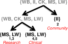
Example 25 (APA election data (continued)).
The APA, as described by Diaconis [1989], is divided into “academicians and clinicians who are on uneasy terms”. In 1980, candidates (W. Bevan and C. Kiesler who were research psychologists) and (M.Siegle and L. Wright, who were clinical psychologists) fell on opposite ends of this political spectrum with candidate 2 (I. Iscoe) being somewhat independent. Diaconis conjectured that voters choose one group over the other, and then choose within. We are now able to verify Diaconis’ conjecture using our riffled independence framework. After removing candidate 2 from the distribution, we perform a search within candidates to again find nearly riffle independent subsets. We find that and are very nearly riffle independent (with respect to KL divergence) and thus are able to verify that candidate sets , , are indeed grouped in a riffle independent sense in the APA data. We remark that in a later work, Marden [1995] identified candidate 2 (I. Iscoe) as belonging to yet a third group of psychologists called community psychologists. The hierarchical structure that best describes the APA data is shown in Figure 8 and the KL-divergence from the true distribution to the hierarchical model is .
Finally for the two main opposing groups within the APA, the riffle shuffling distribution for sets and is not well approximated by a biased riffle shuffle. Instead, since there are two coalitions, we fit a mixture of two biased riffle shuffles to the data and found the bias parameters of the mixture components to be and , indicating that the two components oppose each other (since and lie on either side of ).
7 Structure discovery I: objective functions
Since different hierarchies impose different independence assumptions, we would like to find the structure that is best suited for modeling a given ranking dataset. On some datasets, a natural hierarchy might be available — for example, if one were familiar with the typical politics of APA elections, then it may have been possible to “guess” the optimal hierarchy. However, for general ranked data, it is not always obvious what kind of groupings riffled independence will lead to, particularly for large . Should fruits really be riffle independent of vegetables? Or are green foods riffle independent of red foods?
Over the next three sections, we address the problem of automatically discovering hierarchical riffle independent structures from training data. Key among our observations is the fact that while item ranks cannot be independent due to mutual exclusivity, relative ranks between sets of items are not subject to the same constraints. More than simply being a ‘clustering’ algorithm, however, our procedure can be thought of as a structure learning algorithm, like those from the graphical models literature Koller and Friedman [2009], which find the optimal (riffled) independence decomposition of a distribution.
The base problem that we address in this current section is how to find the best structure if there is only one level of partitioning and two leaf sets, , . Alternatively, we want to find the topmost partitioning of the tree. In Section 8, we use this base case as part of a top-down approach for learning a full hierarchy.
7.1 Problem statement
Given then, a training set of rankings, , , , drawn i.i.d. from a distribution in which a subset of items, , is riffle independent of its complement, , the problem which we address in this section is that of automatically determining the sets and . If does not exactly factor riffle independently, then we would like to find the riffle independent approximation which is closest to in some sense. Formally, we would like to solve the problem:
| (7.1) |
where is the empirical distribution of training examples and is the Kullback-Leibler divergence measure. Equation 7.1 is a seemingly reasonable objective since it can also be interpreted as maximizing the likelihood of the training data. In the limit of infinite data, Equation 7.1 can be shown via the Gibbs inequality to attain its minimum, zero, at the subsets and , if and only if the sets and are truly riffle independent of each other.
For small problems, one can actually solve Problem 7.1 using a single computer by evaluating the approximation quality of each subset and taking the minimum, which was the approach taken in Example 25. However, for larger problems, one runs into time and sample complexity problems since optimizing the globally defined objective function (Equation 7.1) requires relearning all model parameters (, , and ) for each of the exponentially many subsets of . In fact, for large sets and , it is rare that one would have enough samples to estimate the relative ranking parameters and without already having discovered the hierarchical riffle independent decompositions of and . We next propose a more locally defined objective function, reminiscent of clustering, which we will use instead of Equation 7.1. As we show, our new objective will be more tractable to compute and have lower sample complexity for estimation.
7.2 Proposed objective function
The approach we take is to minimize a different measure that exploits the observation that absolute ranks of items in are fully independent of relative ranks of items in , and vice versa (which we prove in Proposition 26). With our vegetables and fruits, for example, knowing that Figs is ranked first among all six items (the absolute rank of a fruit) should give no information about whether Corn is preferred to Peas (the relative rank of vegetables). More formally, given a subset , recall that denotes the vector of (absolute) ranks assigned to items in by (thus, ). We propose to minimize an alternative objective function:
| (7.2) |
where denotes the mutual information (defined between two variables and by .
The function does not have the same likelihood interpretation as the objective function of Equation 7.1. However, it can be thought of as a composite likelihood of two models, one in which the relative rankings of are independent of absolute rankings of , and one in which the relative rankings of are independent of absolute rankings of (see Appendix A.2). With respect to distributions which satisfy (or approximately satisfy) both models (i.e., the riffle independent distributions), minimizing is equivalent to (or approximately equivalent to) maximizing the log likelihood of the data. Furthermore, we can show that is guaranteed to detect riffled independence:
Proposition 26.
is a necessary and sufficient criterion for a subset to be riffle independent of its complement, .
Proof.
Suppose and are riffle independent. We first claim that and are independent. To see this, observe that the absolute ranks of , , are determined by the relative rankings of , and the interleaving . By the assumption that and are riffle independent, we know that the relative rankings of and ( and ), and the interleaving are independent, establishing the claim. The argument that and are independent is similar, thus establishing one direction of the proposition.
To establish the reverse direction, assume that Equation 7.2 evaluates to zero on sets and . It follows that and . Now, as a converse to the observation from above, note that the absolute ranks of determine the relative ranks of , , as well as the interleaving . Similarly, determines and . Thus, and . It then follows that . ∎
As with Equation 7.1, optimizing is still intractable for large . However, motivates a natural proxy, in which we replace the mutual informations defined over all variables by a sum of mutual informations defined over just three variables at a time.
Definition 27 (Tripletwise mutual informations).
Given any triplet of distinct items, , we define the tripletwise mutual information term, .
The tripletwise mutual information can be computed as follows:
where the inside summation runs over two values, true/false, for the binary variable . To evaluate how riffle independent two subsets and are, we want to examine the triplets that straddle the two sets.
Definition 28 (Internal and Cross triplets).
We define to be the set of triplets which “cross” from set to set : is similarly defined. We also define to be the set of triplets that are internal to : and again, is similarly defined.
Our proxy objective function can be written as the sum of the mutual information evaluated over all of the crossing triplets:
| (7.3) |
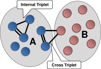
can be viewed as a low order version of , involving mutual information computations over triplets of variables at a time instead of -tuples. The mutual information , for example, reflects how much the rank of a vegetable () tells us about how two fruits (, ) compare. If and are riffle independent, then we know that for any such that , (and similarly for any such that , . Given that fruits and vegetables are riffle independent sets, knowing that Grapes is preferred to Figs should give no information about the absolute rank of Corn, and therefore should be zero. Note that such tripletwise independence assertions bear resemblance to assumptions sometimes made in social choice theory, commonly referred to as Independence of Irrelevant Alternatives [Arrow, 1963], where the addition of a third element , is assumed to not affect whether one prefers an element over .
The objective is somewhat reminiscent of typical graphcut and clustering objectives. Instead of partitioning a set of nodes based on sums of pairwise similarities, we partition based on sums of tripletwise affinities. We show a graphical depiction of the problem in Figure 9, where cross triplets (in , ) have low weight and internal triplets (in , ) have high weight. The objective is to find a partition such that the sum over cross triplets is low. In fact, the problem of optimizing can be seen as an instance of the weighted, directed hypergraph cut problem [Gallo et al., 1993]. Note that the word directed is significant for us, because, unlike typical clustering problems, our triplets are not symmetric (for example, ), resulting in a nonstandard and poorly understood optimization problem.
Example 29 (APA election data (continued)).
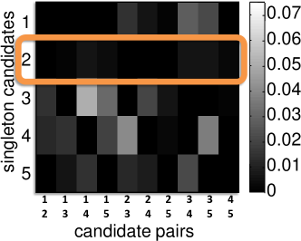
Figure 9 visualizes the tripletwise mutual informations computed from the APA dataset. Since there are five candidates, there are pairs of candidates. The entry in the matrix corresponds to . For easier visualization, we have set entries of the form and to be zero since they are not counted in the objective function.
The highlighted row corresponds to candidate 2, in which all of the mutual information terms are close to zero. We see that the tripletwise mutual information terms tell a story consistent with the conclusion of Example 17, in which we showed that candidate 2 was approximately riffle independent of the remaining candidates.
Finally, it is also interesting to examine the entry. It is the largest mutual information in the matrix, a fact which should not be surprising since candidates 1 and 3 are politically aligned (both research psychologists). Thus, knowing, for example, that candidate 3 was ranked first is a strong indication that candidate 1 was preferred over candidate 4.
7.3 Encouraging balanced partitions
In practice, like the minimum cut objective for graphs, the tripletwise objective of Equation 7.3 has a tendency to “prefer” small partitions (either or very small) to more balanced partitions () due to the fact that unbalanced partitions have fewer triplets that cross between and . The simplest way to avoid this bias is to optimize the objective function over subsets of a fixed size . As we discuss in the next section, optimizing with a fixed can be useful for building thin hierarchical riffle independent models. Alternatively, one can use a modified objective function that encourages more balanced partitions. For example, we have found the following normalized cut [Shi and Malik, 2000] inspired variation of our objective to be useful for detecting riffled independence when the size is unknown:
| (7.4) |
Intuitively, the denominator in Equation 7.4 penalizes subsets whose interiors have small weight. Note that there exist many variations on the objective function that encourage balance, but is the one that we have used in our experiments.
7.4 Low-order detectability assumptions.
When does detect riffled independence? It is not difficult to see, for example, that is a necessary condition for riffled independence, since implies . We have:
Proposition 30.
If and are riffle independent sets, then .
However, the converse of Proposition 30 is not true in full generality without accounting for dependencies that involve larger subsets of variables. Just as the pairwise independence assumptions that are commonly used for randomized algorithms [Motwani and Raghavan, 1996]555 A pairwise independent family of random variables is one in which any two members are marginally independent. Subsets with larger than two members may not necessarily factor independently, however. do not imply full independence between two sets of variables, there exist distributions which “look” riffle independent from tripletwise marginals but do not factor upon examining higher-order terms. Nonetheless, in most practical scenarios, we expect to imply riffled independence.
7.5 Quadrupletwise objective functions for riffled independence
A natural variation of our method is to base the objective function on the following quantities, defined over quadruplets of items instead of triplets:
| (7.5) |
Intuitively, measures how much knowing that, say, Peas is preferred to Corn, tells us about whether Grapes are preferred to Oranges. Again, if the fruits and vegetables are riffle independent, then the mutual information should be zero. Summing over terms which cross between the cut, we obtain a quadrupletwise objective function defined as: If and are riffle independent with and , then the mutual information is zero. Unlike their tripletwise counterparts, however, the do not arise from a global measure that is both necessary and sufficient for detecting riffled independence. In particular, is insufficient to guarantee riffled independence. For example, if the interleaving depends on the relative rankings of and , then riffled independence is not satisfied, yet . Moreover, it is not clear how one would detect riffle independent subsets consisting of a single element using a quadrupletwise measure. As such, we have focused on tripletwise measures in our experiments. Nonetheless, quadrupletwise measures may potentially be useful in practice (for detecting larger subsets) and have the significant advantage that the can be estimated with fewer samples and using almost any imaginable form of partially ranked data.
7.6 Estimating the objective from samples
We have so far argued that is a reasonable function for finding riffle independent subsets. However, since we only have access to samples rather than the true distribution itself, it will only be possible to compute an approximation to the objective . In particular, for every triplet of items, , we must compute an estimate of the mutual information from i.i.d. samples drawn from , and the main question is: how many samples will we need in order for the approximate version of to remain a reasonable objective function?
In the following, we denote the estimated value of by . For each triplet, we use a regularized procedure due to Höffgen [1993] to estimate mutual information. We adapt his sample complexity bound to our problem below.
Lemma 31.
For any fixed triplet , the mutual information can be estimated to within an accuracy of with probability at least using i.i.d. samples and the same amount of time.
The approximate objective function is therefore:
What we want to now show is that, if there exists a unique way to partition into riffle independent sets, then given enough training examples, our approximation uniquely singles out the correct partition as its minimum with high probability. A class of riffle independent distributions for which the uniqueness requirement is satisfied consists of the distributions for which and are strongly connected according to the following definition.
Definition 32.
A subset is called -third-order strongly connected if, for every triplet with distinct, we have .
If a set is riffle independent of and both sets are third order strongly connected, then we can ensure that riffled independence is detectable from third-order terms and that the partition is unique. We have the following probabilistic guarantee.
Theorem 33.
Let and be -third order strongly connected riffle independent sets, and suppose . Given i.i.d. samples, the minimum of is achieved at exactly the subsets and with probability at least .
See the Appendix for details. Finally, we remark that the strong connectivity assumptions used in Theorem 33 are stronger than necessary — and with respect to certain interleaving distributions, it can even be the case that the estimated objective function singles out the correct partition when all of internal triplets belonging to and have zero mutual information. Moreover, in some cases, there are multiple valid partitionings of the item set. For example the uniform distribution is a distribution in which every subset is riffle independent of its complement. In such cases, multiple solutions are equally good when evaluated under , but not its sample approximation, .
8 Structure discovery II: algorithms
Having now designed a function that is tractable to estimate from both perspectives of computational and sample complexity, we turn to the problem of learning the hierarchical riffle independence structure of a distribution from training examples. Instead of directly optimizing an objective in the space of possible hierarchies, we take a simple top-down approach in which the item sets are recursively partitioned by optimizing until some stopping criterion is met (for example, when the leaf sets are smaller than some , or simply stopping after a fixed number of splits).
8.1 Exhaustive optimization
Optimizing the function requires searching through the collection of subsets of size , which, when performed exhaustively, requires time. An exhaustive approach thus runs in exponential time, for example, when .
However, when the size of is known and small (), the optimal partitioning of an item set can be found in polynomial time by exhaustively evaluating over all -subsets.
Corollary 34.
Under the conditions of Theorem 33, one needs at most samples to recover the exact riffle independent partitioning with probability .
When is small, we can therefore use exhaustive optimization to learn the structure of -thin chain models (Section 6.2) in polynomial time. The structure learning problem for thin chains is to discover how the items are partitioned into groups, which group is inserted first, which group is inserted second, and so on. To learn the structure of a thin chain, we can use exhaustive optimization to learn the topmost partitioning of the item set, then recursively learn a thin chain model for the items in the larger subset.
8.2 Handling arbitrary partitions using anchors
When is large, or even unknown, cannot be optimized using exhaustive methods. Instead, we propose a simple algorithm for finding and based on the following observation. If an oracle could identify any two elements of the set , say, , in advance, then the quantity indicates whether the item belongs to or since is nonzero in the first case, and zero in the second case.
For finite training sets, when is only known approximately, one can sort the set and if is known, take the items closest to zero to be the set (when is unknown, one can use a threshold to infer ). Since we compare all items against , we refer to these two fixed items as “anchors”.
Of course are not known in advance, but by fixing to be an arbitrary item, one can repeat the above method for all settings of to produce a collection of candidate partitions. Each partition can then be scored using the approximate objective , and a final optimal partition can be selected as the minimum over the candidates. See Algorithm 4. In cases when is not known a priori, we evaluate partitions for all possible settings of using .
Since the Anchors method does not require searching over subsets, it can be significantly faster than an exhaustive optimization of . Moreover, by assuming -third order strong connectivity as in the previous section, one can use similar arguments to derive sample complexity bounds.
Corollary 35 (of Theorem 33).
Let and be -third order strongly connected riffle independent sets, and suppose . Given i.i.d. samples, the output of the Anchors algorithm is exactly with probability . In particular, the Anchors estimator is consistent.
We remark, however, that there are practical differences that can at times make the Anchors method somewhat less robust than an exhaustive search. Conceptually, anchoring works well when there exists two elements that are strongly connected with all of the other elements in its set, which can then be used as the anchor elements . An exhaustive search can work well in weaker conditions such as when items are strongly connected through longer paths. We show in our experiments that the Anchors method can nonetheless be quite effective for learning hierarchies.
8.3 Running time
We now consider the running time of our structure learning procedures. In both cases, it is necessary to precompute the mutual information quantities for all triplets from samples. For each triplet, we can compute in linear time with respect to the sample size. The set of all triplets can therefore be computed in time.
The exhaustive method for finding the -subset which minimizes requires evaluating the objective function at subsets. What is the complexity of evaluating at a particular partition ? We need to sum the precomputed mutual informations over the number of triangles that cross between and . If and , then we can bound the number of such triangles by . Thus, we require optimization time, leading to a bound of total time.
The Anchors method requires us to (again) precompute mutual informations. The other seeming bottleneck is the last step, in which we must evaluate the objective function at partitions. In reality, if and are both larger than 1, then can be held fixed at any arbitrary element, and we must only optimize over partitions. When , then , in which case the two sets are trivially riffle independent (independent of the actual distribution). As we showed in the previous paragraph, evaluating requires time, and thus optimization using the Anchors method = total time. Since is much smaller than (in any meaningful training set), we can drop it from the big-O notation to get time complexity, showing that the Anchors method is dominated by the time that is required to precompute and cache mutual informations.
9 Structure discovery III: quantifying stability
Given a hierarchy estimated from data, we now discuss how one might practically quantify how confident we should be about the hypothesized structure. We might like to know if the amount of data that was used for estimating the structure was adequate the support the learned structure, and, if the the data looked slightly different, would the hypothesis change?
Bootstrapping [Efron and Tibshirani, 1993] offers a simple approach — repeatedly resample the data with replacement, and estimate a hierarchical structure for each resampling. The difference between our setting and typical bootstrapping settings, however, is that our structures lie in a large discrete set. Thus, unlike continuous parameters, whose confidence we can often summarize with intervals or ellipses, it is not clear how one might compactly summarize a collection of many hierarchical clusterings of items.
The simplest way to summarize the collection of hierarchies obtained via the bootstrap is to measure the fraction of the estimated structures which are identical to the structure estimated from the original unperturbed dataset. If, for small sets of resampled data, the estimated hierarchy is consistently identical to that obtained from the original data, then we can be confident that the data supports the hypothesis. We show in the following example that, for the structure which was learned from the APA dataset, a far smaller dataset would have sufficed.
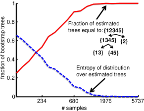
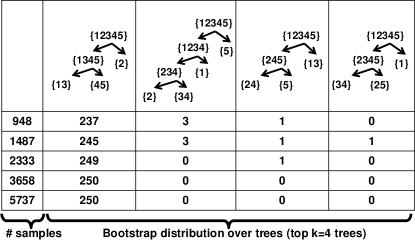
Example 36 (APA Election data (continued)).
As our final APA related example, we show the results of bootstrap resampling in Figure 10. To generate the plots, we resampled the APA dataset with replacement 200 times each for varying sample sizes, and ran our Anchors algorithm on each resulting sample. Figure 10 plots (in solid red) the fraction of bootstrapped trees for each sample size which agree exactly with the hierarchy given in Figure 8. Given that we forced sets to be partitioned until they had at most 2 items, there are 120 possible hierarchical structures for the APA dataset.
It is interesting to see that the hierarchies returned by the algorithm are surprisingly stable even given fewer than 100 samples, with about 25% of bootstrapped trees agreeing with the optimal hierarchy. At 1000 samples, almost all trees agree with the optimal hierarchy. In Figure 10, we show a table of the bootstrap distribution for the largest sample sizes (which were concentrated at only a handful of trees).
For larger item sets , however, it is rarely the case that there is enough data to strongly support the hierarchy in terms of the above measure. In these cases, instead of asking whether entire structures agree with each other exactly, it makes sense to ask whether estimated substructures agree. For example, a simple measure might amount to computing the fraction of structures estimated from resampled datasets which agreed with the original structure at the topmost partition. Another natural measure is to count the fraction of structures which correctly recovered all (or a subset of) leaf sets for the original dataset, but not necessarily the correct hierarchy. By Proposition 23, correctly discovering the leaf set partitioning is probabilistically meaningful, and corresponds to correctly identifying the -way decomposition corresponding to a distribution, but failing to identifying the specific hierarchy.
We remark that sometimes, there is no one unique structure corresponding to a distribution. The uniform distribution, for example, is consistent with any hierarchical riffle independent structure, and so bootstrapped hierarchies will not concentrate on any particular structure or even substructure. Moreover, even when there is true unique structure corresponding to the generating distribution, it may be the case that other simpler structures perform better when there is not much available training data.
10 Related work
Our work draws from several literatures: card shuffling research due primarily to Persi Diaconis and collaborators [Bayer and Diaconis, 1992; Fulman, 1998], papers about Fourier theoretic probabilistic inference over permutations from the machine learning community[Kondor, 2008; Huang, Guestrin and Guibas, 2009b; Huang et al., 2009], as well as graphical model structure learning research.
10.1 Card shuffling theory
Bayer and Diaconis [1992] provided a a convergence analysis of repeated riffle shuffles. Our novelty lies in the combination of shuffling theory with independence, which was first exploited in Huang et al. [2009], for scaling inference operations to large problems. Finally, we remark that Fulman [1998] introduced a class of shuffles known as biased riffle shuffles which are not the same as the biased riffle shuffles discussed in our paper. The fact that the uniform riffle shuffling can be realized by dropping card with probability proportional to the number of cards remaining in each hand has been observed in a number of papers [Bayer and Diaconis, 1992], but we are the first to (1) formalize this in the form of the recurrence given in Equation C.1, and (2) to compute the Fourier transform of the uniform and biased riffle shuffling distributions.
10.2 Fourier analysis on permutations
Our dynamic programming approach bears some similarities to the FFT (Fast Fourier Transform) algorithm proposed by Clausen and Baum [1993], and in particular, relies on the same branching rule recursions [Sagan, 2001]. While the Clausen FFT requires time, since our biased riffle shuffles are parameterized by a single , we can use the recurrence to compute low-frequency Fourier terms in polynomial time.
10.3 Learning structured representations
Our insights for the structure learning problems are inspired by some of the recent approaches in the machine learning literature for learning the structure of thin junction trees [Bach and Jordan, 2001]. In particular, the idea of using a low order proxy objective with a graph-cut like optimization algorithm is similar to an idea which was recently introduced in Shahaf, Chechetka and Guestrin [2009], which determines optimally thin separators with respect to the Bethe free energy approximation (of the entropy) rather than a typical log-likelihood objective. Our sample analysis is based on the mutual information sample complexity bounds derived in Höffgen [1993], which was also used in Chechetka and Guestrin [2007] for developing a structure learning algorithm for thin junction trees with provably polynomial sample complexity. Finally, the bootstrap methods which we have employed in our experiments for verifying robustness bear much resemblance to some of the common bootstrapping methods which have been used in bioinformatics for analyzing phylogenetic trees [Holmes, 1999, 2003].
11 Experiments
In this section, we present a series of experiments to validate our models and methods. All experiments were implemented in Matlab, except for the Fourier theoretic routines, which were written in C++. We tested on lab machines with two AMD quadcore Opteron 2.7GHz processors with 32 Gb memory. We have already analyzed the APA data extensively throughout the paper. Here, we demonstrate our algorithms on simulated data as well as other real datasets, namely, sushi preference data, and Irish election data.
11.1 Simulated data
We begin with a discussion of our simulated data experiments. We first consider approximation quality and timing issues for a single binary partition of the item set.
Binary partitioning of the item set
To understand the behavior of RiffleSplit in approximately riffle independent situations, we drew sample sets of varying sizes from a riffle independent distribution on (with bias parameter ) and use RiffleSplit to estimate the relative ranking factors and interleaving distribution from the empirical distribution. In Figure 11(a), we plot the KL-divergence between the true distribution and that obtained by applying RiffleJoin to the estimated riffle factors. With small sample sizes (far less than ), we are able to recover accurate approximations despite the fact that the empirical distributions are not exactly riffle independent. For comparison, we ran the experiment using the Split algorithm Huang et al. [2009] to recover the parameters. Perhaps surprisingly, one can show that the Split algorithm from Huang et al. [2009] is also an unbiased, consistent estimator of the riffle factors, but it does not return the maximum likelihood parameter estimates because it effectively ignores rankings which are not contained in the subgroup . Consequently, our RiffleSplit algorithm converges to the correct parameters with far fewer samples.
Next, we show that our Fourier domain algorithms are capable of handling sizeable item sets (with size ) when working with low-order terms. In Figure 11(b) we ran our Fourier domain RiffleJoin algorithm on various simulated distributions. We plot running times of RiffleJoin (without precomputing the interleaving distributions) as a function of (setting , which is the worst case) scaling up to .
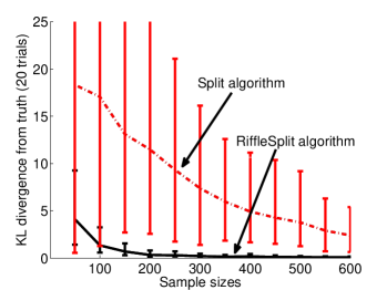
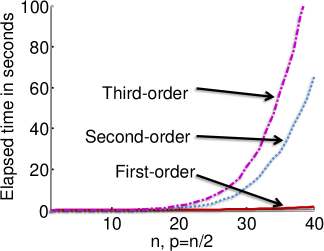
Learning a hierarchy of items
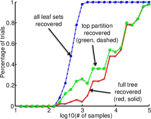
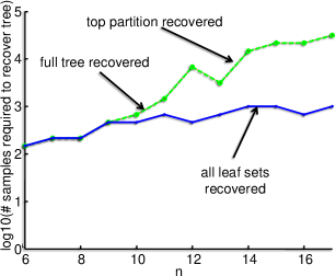
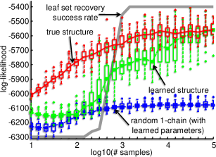
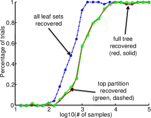
We next applied our methods to synthetic data to show that, given enough samples, our algorithms do effectively recover the optimal hierarchical structures which generated the original datasets. For various settings of , we simulated data drawn jointly from a -thin chain model (for ) with a random parameter setting for each structure and applied our exact method for learning thin chains to each sampled dataset. First, we investigated the effect of varying sample size on the proportion of trials (out of fifty) for which our algorithms were able to (a) recover the full underlying tree structure exactly, (b) recover the topmost partition correctly, or (c) recover all leaf sets correctly (but possibly out of order). Figure 12(a) shows the result for an itemset of size . Figure 12(b), shows, as a function of , the number of samples that were required in the same experiments to (a) exactly recover the full underlying structure or (b) recover the correct leaf sets, for at least 90% of the trials. What we can observe from the plots is that, given enough samples, reliable structure recovery is indeed possible. It is also interesting to note that recovery of the correct leaf sets can be done with much fewer samples than are required for recovering the full hierarchical structure of the model.
After learning a structure for each dataset, we learned model parameters and evaluated the log-likelihood of each model on 200 test examples drawn from the true distributions. In Figure 12(c), we compare log-likelihood performance when (a) the true structure is given (but not parameters), (b) a -thin chain is learned with known , and (c) when we use a random generated 1-chain structure. As expected, knowing the true structure results in the best performance, and the 1-chain is overconstrained. However, our structure learning algorithm is eventually able to catch up to the performance of the true structure given enough samples. It is also interesting to note that the jump in performance at the halfway point in the plot coincides with the jump in the success rate of discovering all leaf sets correctly — we conjecture that performance is sometimes less sensitive to the actual hierarchy used, as long as the leaf sets have been correctly discovered.
To test the Anchors algorithm, we ran the same simulation using Algorithm 4 on data drawn from hierarchical models with no fixed . We generated roughly balanced structures, meaning that item sets were recursively partitioned into (almost) equally sized subsets at each level of the hierarchy. From Figure 12(d), we see that the Anchors algorithm can also discover the true structure given enough samples. Interestingly, the difference in sample complexity for discovering leaf sets versus discovering the full tree is not nearly as pronounced as in Figure 12(a). We believe that this is due to the fact that the balanced trees have less depth than the thin chains, leading to fewer opportunities for our greedy top-down approach to commit errors.
11.2 Data analysis: sushi preference data
We now turn to analyzing real datasets. For our first analysis, we examine a sushi preference ranking dataset [Kamishima, 2003] consisting of 5000 full rankings of ten types of sushi. The items are enumerated in Figure 13. Note that, compared to the APA election data, the sushi dataset has twice as many items, but fewer examples.
| 1. ebi (shrimp) | 2. anago (sea eel) | 3. maguro (tuna) |
| 4. ika (squid) | 5. uni (sea urchin) | 6. sake (salmon roe) |
| 7. tamago (egg) | 8. toro (fatty tuna) | 9. tekka-maki (tuna roll) |
| 10. kappa-maki (cucumber roll) |
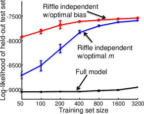
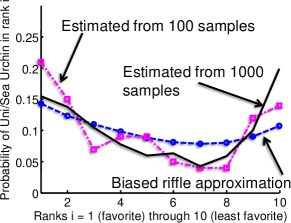
We begin by studying our methods in the case of a single binary partitioning of the item set. Unlike the APA dataset, there is no obvious way to naturally partition the types of sushi into two sets — in our first set of experiments, we have arbitrarily divided the item set into and .
We divided the data into training and test sets (with 500 examples) and estimated the true distribution in three ways: (1) directly from samples (with regularization), (2) using a riffle independent distribution (split evenly into two groups of five and mentioned above) with the optimal shuffling distribution , and (3) with a biased riffle shuffle (and optimized bias ). Figure 14(a) plots testset log-likelihood as a function of training set size — we see that riffle independence assumptions can help significantly to lower the sample complexity of learning. Biased riffle shuffles, as can also be seen, are a useful learning bias with very small samples.
As an illustration of the behavior of biased riffle shuffles, see Figure 14(b) which shows the approximate first-order marginals of Uni (Sea Urchin) rankings, and the biased riffle approximation. The Uni marginals are interesting, because while many people like Uni, thus providing high rankings, many people also hate it, providing low rankings. The first-order marginal estimates have significant variance at low sample sizes, but with the biased riffle approximation, one can achieve a reasonable approximation to the distribution even with few samples at the cost of being somewhat oversmoothed.
Structure learning on the sushi dataset
Figure 16(b) shows the hierarchical structure that we learn using the entire sushi dataset. Since the sushi are not prepartitioned into distinct coalitions, it is somewhat more difficult than with, say, the APA data, to interpret whether the estimated structure makes sense. However, parts of the tree certainly seem like reasonable groupings. For example, all of the tuna related sushi types have been clustered together. Tamago and kappa-maki (egg and cucumber rolls) are “safer”, typically more boring choices, while uni and sake (sea urchin and salmon roe) are more daring. Anago (sea eel), is the odd man out in the estimated hierarchy, being partitioned away from the remaining items at the top of the tree.
To understand the behavior of our algorithm with smaller sample sizes, we looked for features of the tree from Figure 16(b) which remained stable even when learning with smaller sample sizes. Figure 16(a) summarizes the results of our bootstrap analysis for the sushi dataset, in which we resample from the original training set 200 times at each of different sample sizes and plot the proportion of learned hierarchies which, (a) recover ‘sea eel’ as the topmost partition, (b) recover all leaf sets correctly, (c), recover the entire tree correctly, (d) recover the tuna-related sushi leaf set, (e) recover the {tamago, kappa-maki} leaf set, and (f) recover the {uni, sake} leaf set.
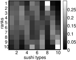
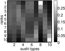
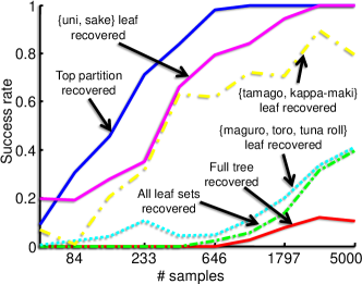
11.3 Data analysis: Irish election data
We next applied our algorithms to a larger Irish House of Parliament (Dáil Éireann) election dataset from the Meath constituency in Ireland (Figure 17(a)). The Dáil Éireann uses the single transferable vote (STV) election system, in which voters rank a subset of candidates. In the Meath constituency, there were 14 candidates in the 2002 election, running for five allotted seats. The candidates identified with the two major rival political parties, Fianna Fáil and Fine Gael, as well as a number of smaller parties (Figure 17(b)). See Gormley and Murphy [2006] for more election details (including candidate names) as well as an alternative analysis. In our experiments, we used a subset of roughly 2500 fully ranked ballots from the election.
Candidate Party 1 Brady, J. Fianna Fáil 2 Bruton, J. Fine Gael 3 Colwell, J. Independent 4 Dempsey, N. Fianna Fáil 5 English, D. Fine Gael 6 Farrelly, J. Fine Gael 7 Fitzgerald, B. Independent 8 Kelly, T. Independent 9 O’Brien, P. Independent 10 O’Byrne, F. Green Party 11 Redmond, M. Christian Solidarity 12 Reilly, J. Sinn Féin 13 Wallace, M. Fianna Fáil 14 Ward, P. Labour
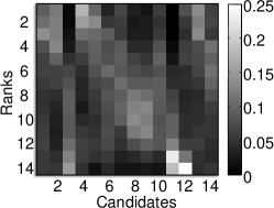
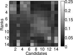
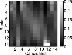
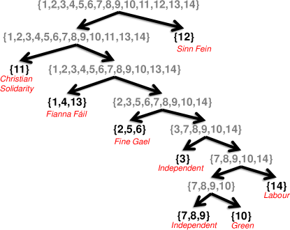
To summarize the dataset, Figure 18(a) shows the matrix of first-order marginals estimated from the dataset. Candidates form the set of “major” party candidates belonging to either Fianna Fáil or Fine Gael, and as shown in the figure, fared much better in the election than the other seven minor party candidates. Notably, candidates 11 and 12 (belonging to the Christian Solidary Party and Sinn Féin, respectively) received on average, the lowest ranks in the 2002 election. One of the differences between the two candidates, however, is that a significant portion of the electorate also ranked the Sinn Féin candidate very high.
Though it may not necessarily be clear how one might partition the candidates, a natural idea might be to assume that the major party candidates () are riffle independent of the minor party candidates (). In Figure 18(b), we show the first-order marginals corresponding to an approximation in which and are assumed to be riffle independent. Visually, the approximate first-order marginals can be seen to be roughly similar to the exact first-order marginals, however there are significant features of the matrix which are not captured by the approximation — for example, the columns belonging to candidates 11 and 12 are not well approximated. In Figure 18(c), we plot a more principled approximation corresponding to a learned hierarchy, which we discuss next. As can be seen, the first-order marginals obtained via structure learning is visually much closer to the exact marginals.
Structure discovery on the Irish election data
As with the APA data, both the exhaustive optimization of and the Anchors algorithm returned the same tree, with running times of 69.7 seconds and 2.1 seconds respectively (not including the 3.1 seconds required for precomputing mutual informations). The resulting tree, with candidates enumerated alphabetically from 1 through 14, is shown (only up to depth 4), in Figure 19. As expected, the candidates belonging to the two major parties, Fianna Fáil and Fine Gael, are neatly partitioned into their own leaf sets. The topmost leaf is the Sinn Fein candidate, indicating that voters tended to insert him into the ranking independently of all of the other 13 candidates.
To understand the behavior of our algorithm with smaller sample sizes, we looked for features of the tree from Figure 19 which remained stable even when learning with smaller sample sizes. In Figure 20(a), we resampled from the original training set 200 times at different sample sizes and plot the proportion of learned hierarchies which, (a) recover the Sinn Fein candidate as the topmost leaf, (b) partition the two major parties into leaf sets, and (c) agree with the original tree on all leaf sets, and (d) recover the entire tree. Note that while the dataset is insufficient to support the entire tree structure, even with about 100 training examples, candidates belonging to the major parties are consistently grouped together indicating strong party influence in voting behavior.
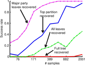
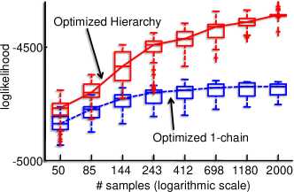
We compared the results between learning a general hierarchy (without fixed ) and learning a 1-thin chain model on the Irish data. Figure 20(b) shows the log-likelihoods achieved by both models on a held-out test set as the training set size increases. For each training set size, we subsampled the Irish dataset 100 times to produce confidence intervals. Again, even with small sample sizes, the hierarchy outperforms the 1-chain and continually improves with more and more training data. One might think that the hierarchical models, which use more parameters are prone to overfitting, but in practice, the models learned by our algorithm devote most of the extra parameters towards modeling the correlations among the two major parties. As our results suggest, such intraparty ranking correlations are crucial for achieving good modeling performance.
Finally, we ran our structure learning algorithm on two similar but smaller election datasets from the other constituencies in the 2002 election which supported electronic voting, the Dublin North and West constituencies. Figure 21 shows the resulting hierarchies learned from each dataset. As with the Meath constituency, the Fianna Fáil and Fine Gael are consistently grouped together in leaf sets in the Dublin datasets. Interestingly, the Sinn Féin and Socialist parties are also consistently grouped in the Dublin datasets, potentially indicating some latent similarities between the two parties.
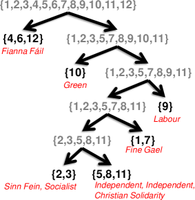
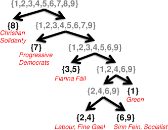
12 Conclusions
Exploiting independence structure for efficient inference and low sample complexity is a simple yet powerful idea, pervasive throughout the machine learning literature, showing up in the form of Bayesian networks, Markov random fields, and more. For rankings, independence can be problematic due to mutual exlusivity constraints, and we began our paper by indicating a need for a useful generalization of independence.
The main contribution of our paper is the definition of such a generalized notion, namely, riffled independence. There are a number of natural questions that immediately follow any such definition, such as:
-
•
Does the generalization retain any of the computational advantages of probabilistic independence?
-
•
Can we find evidence that such generalized independence relations hold (or approximately hold) in real datasets?
-
•
If subsets of items in a ranking dataset indeed satisfy the generalized independence assumption, or approximately so, how could we algorithmically determine what these subsets should be from samples?
We have shown that for riffled independence, the answer to each of the above questions lies in the affirmative. We next explored hierarchical riffle independent decompositions. Our model, in which riffle independent subsets are recursively chained together, leads to a simple, interpretable model whose structure we can estimate from data, and we have successfully applied our learning algorithms to several real datasets.
Currently, the success of our structure learning methods depends on the existence of a fairly sizeable dataset of full rankings. However, ranking datasets are more typically composed of partial or incomplete rankings, which are often far easier to elicit from a multitude of users. For example, top- type rankings, or even rating data (in which a user/judge provides a rating of an item between, say, 1 and 5) are common. Extending our parameter and structure learning algorithms for handling such partially ranked data would be a valuable and practical extension of our work. For structure learning, our tripletwise mutual information measures can already potentially be estimated within a top- ranking setting. It would be interesting to also develop methods for estimating these mutual information measures from other forms of partial rankings. Additionally, the effect of using partial rankings on structure learning sample complexity is not yet understood, and the field would benefit from a careful analysis.
Many other possible extensions are possible. In our paper, we have developed algorithms for estimating maximum likelihood parameters. For small training set sizes, a Bayesian approach would be more appropriate, where a prior is placed on the parameter space. However, if the prior distribution ties parameters together (i.e., if the prior does not factor across parameters), then the structure learning problem can be considerably more complicated, since we would not be able to simply identify independence relations.
Riffled independence is a new tool for analyzing ranked data and as we have shown, has the potential to give new insights into ranking datasets. We strongly believe that it will be crucial in developing fast and efficient inference and learning procedures for ranking data, and perhaps other forms of permutation data.
Acknowledgements
This work is supported in part by the ONR under MURI N000140710747, and the Young Investigator Program grant N00014-08-1-0752. We thank Khalid El-Arini for feedback on initial drafts, and Brendan Murphy and Claire Gormley for providing the Irish voting datasets. Discussions with Marina Meila provided valuable initial ideas upon which this work is based.
Appendix A More proofs and discussion
A.1 Proof of Lemma 14
Proof.
Let be an item in (with ). Since , is some number between and . By definition, for any the interleaving map returns the largest rank in . Thus, is the -th largest rank in , which is simply the absolute rank of item . Therefore, we conclude that . Similarly, if , we have (the added is necessary since the indices of are offset by in ), and we can conclude that . ∎
A.2 Log-likelihood interpretations
If we examine the KL divergence objective introduced in Section 7, it is a standard fact that minimizing Equation 7.1 is equivalent to find the structure which maximizes the log-likelihood of the training data.
In the above (with some abuse of notation), , and are estimated using counts from the training data. The equivalence is significant because it justifies structure learning for data which is not necessarily generated from a distribution which factors into riffle independent components. Using a similar manipulation, we can rewrite our objective function (Equation 7.2) as:
which we can see to be a “composite” of two likelihood functions. We are evaluating our data log-likelihood first under a model in which the absolute ranks of items in are independent of relative ranks of items in , and secondly under a model in which the absolute ranks of items in are independent of relative ranks of items in . Here again, and are estimated using counts of the training data. We see that if these distributions, , factor along their inputs, then optimizing the objective function is equivalent to optimizing the likelihood under the riffle independent model. Thus, if the data is already riffle independent (or nearly riffle independent), then the structure learning objective can indeed to be interpreted as maximizing the log-likelihood of the data, but otherwise there does not seem to be a clear equivalence between the two objective functions.
A.3 Why testing for independence of relative ranks is insufficient
Why can we not just check to see that the relative ranks of are independent of the relative ranks of ? Another natural objective function for detecting riffle independent subsets is:
| (A.1) |
Equation A.1 is certainly a necessary condition for subsets and to be riffle independent but why would it not be sufficient? It is easy to construct a counterexample — simply find a distribution in which the interleaving depends on either of the relative rankings.
Example 37.
In this example, we will consider a distribution on . Let and . To generate rankings , we will draw independent relative rankings, and , with uniform probability for each of and . Then set the interleaving as follows:
Finally set .
Since the relative rankings are independent, . But since the interleaving depends on the relative ranking of items in , we see that and are not riffle independent in this example.
Appendix B Manipulating interleaving distributions in the Fourier domain
Appendix C Proof of recurrence
Theorem 38.
Algorithm 1 returns a uniformly distributed -interleaving.
Proof.
The proof is by induction on . The base case (when ) is obvious since the algorithm can only return a single permutation.
Next, we assume for the sake of induction that for any , the algorithm returns a uniformly distributed interleaving and we want to show this to also be the case for .
Let be any interleaving in . We will show that . Consider . There are two cases: is either a -interleaving (in which case ), or a -interleaving (in which case ).
We will just consider the first case since the second is similar. is uniformly distributed by the inductive hypothesis and therefore has probability .
is set to independently with probability , so we compute the probability of the interleaving resulting from the algorithm as:
∎
Fourier transforming the biased riffle shuffle
We describe the recurrence satisfied by , allowing one to write , a distribution on , in terms of and , distributions over (see Algorithm in main paper). Given a function , we will define the embedded function by if , and otherwise. Algorithm 1 can be then rephrased as a recurrence relation as follows.
Proposition 39.
The uniform riffle shuffling distribution obeys the recurrence relation:
| (C.1) |
with base cases: , where is the delta function at the identity permutation.
Note that by taking the support sizes of each of the functions in the above recurrence, we recover the following well known recurrence for binomial coefficients:
| (C.2) |
The biased riffle shuffle is defined by:
| (C.3) |
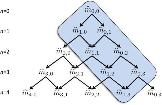
Writing the recursion in the form of Equation C.1 provides a construction of the uniform riffle shuffle as a sequence of operations on smaller distribution which can be performed completely with respect to Fourier coefficients. In particular, given the Fourier coefficients of a function , one can construct the Fourier coefficients of the embedding by applying the branching rule (see Sagan [2001]; Kondor and Borgwardt [2008] for details). Using the linearity property, the Convolution Theorem 20 and the fact that embeddings can be performed in the Fourier domain, we arrive at the equivalent Fourier-theoretic recurrence for each frequency level .
| (C.4) |
where is the irreducible representation matrix evaluated at the cycle (see Huang, Guestrin and Guibas [2009b] for details on irreducible representations). Implementing the recurrence (Equation C.4) in code can naively result in an exponential time algorithm if one is not careful. It is necessary to use dynamic programming to be sure not to recompute things that were already computed. In Algorithm 5, we present pseudocode of such a dynamic programming approach, which builds a ‘Pascal’s triangle’ similar to that which might be constructed to compute a table of binomial coefficients. The pseudocode assumes the existence of Fourier domain algorithms for convolving distributions and for embedding a distribution over into . See Figure 22 for a graphical illustration of the algorithm.
C.1 Sample complexity analysis
Lemma 40 (adapted from Höffgen [1993]).
The entropy of a discrete random variable with arity can be estimated to within accuracy with probability using i.i.d samples and the same time.
Lemma 41.
The collection of mutual informations can be estimated to within accuracy for all triplets with probability at least using i.i.d. samples and the same amount of time.
Proof.
Fix a and . For any fixed triplet , Hoffgen’s result (Lemma 40) implies that can be estimated with accuracy with probability at least using i.i.d. samples since the variable has arity and setting .
Estimating the mutual information for the same triplet therefore requires the same sample complexity by the expansion: . Now we use a simple union bound to bound the probability that the collection of mutual informations over all triplets is estimated to within accuracy. Define .
∎
Lemma 42.
Fix . and let be a -subset of with riffle independent of its complement . Let be a -subset with or . If and are each -third order strongly connected, we have , where .
Proof.
Let us first establish some notation. Given a subset , define
Thus and are the sets of triplets whose indices are all internal to or internal to respectively. We define to be the set of triplets which “cross” between the sets and :
The goal of this proof is to use the strong connectivity assumptions to lower bound . In particular, due to strong connectivity, each triplet inside that also lies in either or must contribute at least to the objective function . It therefore suffices to lower bound the number of triplets which cross between and , but are internal to either or (i.e., ). Define and note that . It is straightforward to check that: , , and .
We do want the bound above to depend on . Intuitively, for a fixed and , the above expression is minimized when either or (a more formal argument is shown below in the proof of Lemma 43). Plugging and and bounding from below yields:
Finally due to strong connectivity, we know that for each triplet in , we have , thus each edge in contributes at least to , establishing the desired result. ∎
Lemma 43.
Under the same assumptions as Lemma 42, is minimized at either or .
Proof.
Let . We know that since by assumption (and equals zero only when ). We want to find the which minimizes the concave quadratic function , the roots of which are and (note that . The minimizer is thus the element of which is closest to either of the roots. ∎
Theorem 44.
Let be a -subset of with riffle independent of its complement . If and are each -third order strongly connected, then given i.i.d. samples, the minimum of (evaluated over all -subsets of ) is achieved at exactly the subsets and with probability at least .
Proof.
Let be a -subset with or . Our goal is to show that .
Denote the error between estimated mutual information and true mutual information by . We have:
| (by Lemma 42 and ) |
Now assume that all of the estimation errors are uniformly bounded as:
| (C.5) |
And note that . We have:
Combining this bound on the estimation errors with the bound on yields:
which is almost what we want to show. How many samples do we require to achieve the bound assumed in Equation C.5 with high probability? Observe that the bound simplifies as,
References
- Arrow [1963] {bbook}[author] \bauthor\bsnmArrow, \bfnmKenneth\binitsK. (\byear1963). \btitleSocial Choice and Individual Values. \bpublisherYale University Press. \endbibitem
- Bach and Jordan [2001] {binproceedings}[author] \bauthor\bsnmBach, \bfnmFrancis R.\binitsF. R. and \bauthor\bsnmJordan, \bfnmMichael I.\binitsM. I. (\byear2001). \btitleThin Junction Trees. In \bbooktitleAdvances in Neural Information Processing Systems 14 \bpages569–576. \bpublisherMIT Press. \endbibitem
- Bayer and Diaconis [1992] {barticle}[author] \bauthor\bsnmBayer, \bfnmD.\binitsD. and \bauthor\bsnmDiaconis, \bfnmP.\binitsP. (\byear1992). \btitleTrailing the Dovetail Shuffle to its Lair. \bjournalThe Annals of Probability. \endbibitem
- Chechetka and Guestrin [2007] {binproceedings}[author] \bauthor\bsnmChechetka, \bfnmA.\binitsA. and \bauthor\bsnmGuestrin, \bfnmC.\binitsC. (\byear2007). \btitleEfficient Principled Learning of Thin Junction Trees. In \bbooktitleNIPS. \endbibitem
- Chen et al. [2009] {binproceedings}[author] \bauthor\bsnmChen, \bfnmHarr\binitsH., \bauthor\bsnmBranavan, \bfnmS. R. K.\binitsS. R. K., \bauthor\bsnmBarzilay, \bfnmRegina\binitsR. and \bauthor\bsnmKarger, \bfnmDavid R.\binitsD. R. (\byear2009). \btitleGlobal models of document structure using latent permutations. In \bbooktitleNAACL 2009 \bpages371–379. \bpublisherAssociation for Computational Linguistics. \endbibitem
- Clausen and Baum [1993] {barticle}[author] \bauthor\bsnmClausen, \bfnmMichael\binitsM. and \bauthor\bsnmBaum, \bfnmUlrich\binitsU. (\byear1993). \btitleFast Fourier Transforms for Symmetric Groups: Theory and Implementation. \bjournalMathematics of Computations \bvolume61 \bpages833-847. \endbibitem
- Diaconis [1988] {bbook}[author] \bauthor\bsnmDiaconis, \bfnmP.\binitsP. (\byear1988). \btitleGroup Representations in Probability and Statistics. \bpublisherIMS Lecture Notes. \endbibitem
- Diaconis [1989] {barticle}[author] \bauthor\bsnmDiaconis, \bfnmP.\binitsP. (\byear1989). \btitleA Generalization of Spectral Analysis with Application to Ranked Data. \bjournalThe Annals of Statistics \bvolume17 \bpages949-979. \endbibitem
- Efron and Tibshirani [1993] {bbook}[author] \bauthor\bsnmEfron, \bfnmBradley\binitsB. and \bauthor\bsnmTibshirani, \bfnmRobert\binitsR. (\byear1993). \btitleAn introduction to the bootstrap. \bpublisherChapman and Hall, London. \endbibitem
- Farias, Jagabathula and Shah [2009] {bincollection}[author] \bauthor\bsnmFarias, \bfnmVivek\binitsV., \bauthor\bsnmJagabathula, \bfnmSrikanth\binitsS. and \bauthor\bsnmShah, \bfnmDevavrat\binitsD. (\byear2009). \btitleA Data-Driven Approach to Modeling Choice. In \bbooktitleAdvances in Neural Information Processing Systems 22 (\beditor\bfnmY.\binitsY. \bsnmBengio, \beditor\bfnmD.\binitsD. \bsnmSchuurmans, \beditor\bfnmJ.\binitsJ. \bsnmLafferty, \beditor\bfnmC. K. I.\binitsC. K. I. \bsnmWilliams and \beditor\bfnmA.\binitsA. \bsnmCulotta, eds.) \bpages504–512. \endbibitem
- Fligner and Verducci [1986] {barticle}[author] \bauthor\bsnmFligner, \bfnmMichael\binitsM. and \bauthor\bsnmVerducci, \bfnmJoseph\binitsJ. (\byear1986). \btitleDistance-based Ranking models. \bjournalJournal of the Royal Statistical Society, Series B \bvolume83 \bpages859-869. \endbibitem
- Fligner and Verducci [1988] {barticle}[author] \bauthor\bsnmFligner, \bfnmM.\binitsM. and \bauthor\bsnmVerducci, \bfnmJ.\binitsJ. (\byear1988). \btitleMulistage Ranking Models. \bjournalJournal of the American Statistical Association \bvolume83. \endbibitem
- Fulman [1998] {barticle}[author] \bauthor\bsnmFulman, \bfnmJ.\binitsJ. (\byear1998). \btitleThe combinatorics of biased riffle shuffles. \bjournalCombinatorica \bvolume18 \bpages173-184. \endbibitem
- Gallo et al. [1993] {barticle}[author] \bauthor\bsnmGallo, \bfnmG.\binitsG., \bauthor\bsnmLongo, \bfnmG.\binitsG., \bauthor\bsnmPallottino, \bfnmS.\binitsS. and \bauthor\bsnmNguyen, \bfnmS.\binitsS. (\byear1993). \btitleDirected hypergraphs and applications. \bjournalDiscrete Appl. Math. \bvolume42. \endbibitem
- Gormley and Murphy [2006] {binproceedings}[author] \bauthor\bsnmGormley, \bfnmC.\binitsC. and \bauthor\bsnmMurphy, \bfnmB.\binitsB. (\byear2006). \btitleA Latent Space Model for Rank Data. In \bbooktitleICML. \endbibitem
- Guiver and Snelson [2009] {binproceedings}[author] \bauthor\bsnmGuiver, \bfnmJohn\binitsJ. and \bauthor\bsnmSnelson, \bfnmEdward\binitsE. (\byear2009). \btitleBayesian inference for Plackett-Luce ranking models. In \bbooktitleICML. \endbibitem
- Helmbold and Warmuth [2007] {binproceedings}[author] \bauthor\bsnmHelmbold, \bfnmD. P.\binitsD. P. and \bauthor\bsnmWarmuth, \bfnmM. K.\binitsM. K. (\byear2007). \btitleLearning Permutations with Exponential Weights. In \bbooktitleCOLT. \endbibitem
- Höffgen [1993] {binproceedings}[author] \bauthor\bsnmHöffgen, \bfnmK. U.\binitsK. U. (\byear1993). \btitleLearning and Robust Learning of Product Distributions. In \bbooktitleCOLT. \endbibitem
- Holmes [1999] {barticle}[author] \bauthor\bsnmHolmes, \bfnmSusan\binitsS. (\byear1999). \btitlePhylogenies: an overview. \bjournalIMA series, Statistics and Genetics \bvolume112 \bpages81-119. \endbibitem
- Holmes [2003] {barticle}[author] \bauthor\bsnmHolmes, \bfnmSusan\binitsS. (\byear2003). \btitleBootstrapping phylogenetic trees: theory and methods. \bjournalStatistical Science \bvolume18 \bpages241-255. \endbibitem
- Huang, Guestrin and Guibas [2007] {binproceedings}[author] \bauthor\bsnmHuang, \bfnmJ.\binitsJ., \bauthor\bsnmGuestrin, \bfnmC.\binitsC. and \bauthor\bsnmGuibas, \bfnmL.\binitsL. (\byear2007). \btitleEfficient Inference for Distributions on Permutations. In \bbooktitleNIPS. \endbibitem
- Huang and Guestrin [2009a] {binproceedings}[author] \bauthor\bsnmHuang, \bfnmJ.\binitsJ. and \bauthor\bsnmGuestrin, \bfnmC.\binitsC. (\byear2009a). \btitleRiffled Independence for Ranked Data. In \bbooktitleNIPS. \endbibitem
- Huang, Guestrin and Guibas [2009b] {barticle}[author] \bauthor\bsnmHuang, \bfnmJ.\binitsJ., \bauthor\bsnmGuestrin, \bfnmC.\binitsC. and \bauthor\bsnmGuibas, \bfnmL.\binitsL. (\byear2009b). \btitleFourier theoretic probabilistic inference over permutations. \bjournalJMLR \bvolume10. \endbibitem
- Huang and Guestrin [2010] {binproceedings}[author] \bauthor\bsnmHuang, \bfnmJ.\binitsJ. and \bauthor\bsnmGuestrin, \bfnmC.\binitsC. (\byear2010). \btitleLearning Hierarchical Riffle Independent Groupings from Rankings. In \bbooktitleICML. \endbibitem
- Huang et al. [2009] {binproceedings}[author] \bauthor\bsnmHuang, \bfnmJ.\binitsJ., \bauthor\bsnmGuestrin, \bfnmC.\binitsC., \bauthor\bsnmJiang, \bfnmX.\binitsX. and \bauthor\bsnmGuibas, \bfnmL.\binitsL. (\byear2009). \btitleExploiting Probabilistic Independence for Permutations. In \bbooktitleAISTATS. \endbibitem
- Jagabathula and Shah [2008] {binproceedings}[author] \bauthor\bsnmJagabathula, \bfnmS.\binitsS. and \bauthor\bsnmShah, \bfnmD.\binitsD. (\byear2008). \btitleInferring rankings under constrained sensing. In \bbooktitleNIPS. \endbibitem
- Kamishima [2003] {binproceedings}[author] \bauthor\bsnmKamishima, \bfnmT.\binitsT. (\byear2003). \btitleNantonac collaborative filtering: recommendation based on order responses. In \bbooktitleKDD \bpages583–588. \endbibitem
- Koller and Friedman [2009] {bbook}[author] \bauthor\bsnmKoller, \bfnmD.\binitsD. and \bauthor\bsnmFriedman, \bfnmN.\binitsN. (\byear2009). \btitleProbabilistic Graphical Models: Principles and Techniques. \bpublisherMIT Press. \endbibitem
- Kondor [2008] {bphdthesis}[author] \bauthor\bsnmKondor, \bfnmR.\binitsR. (\byear2008). \btitleGroup Theoretical Methods in Machine Learning \btypePhD thesis, \bschoolColumbia University. \endbibitem
- Kondor and Borgwardt [2008] {binproceedings}[author] \bauthor\bsnmKondor, \bfnmR.\binitsR. and \bauthor\bsnmBorgwardt, \bfnmK. M.\binitsK. M. (\byear2008). \btitleThe skew spectrum of graphs. In \bbooktitleICML \bpages496-503. \endbibitem
- Kondor, Howard and Jebara [2007] {binproceedings}[author] \bauthor\bsnmKondor, \bfnmR.\binitsR., \bauthor\bsnmHoward, \bfnmA.\binitsA. and \bauthor\bsnmJebara, \bfnmT.\binitsT. (\byear2007). \btitleMulti-Object Tracking with Representations of the Symmetric Group. In \bbooktitleAISTATS. \endbibitem
- Lebanon and Mao [2008] {binproceedings}[author] \bauthor\bsnmLebanon, \bfnmG.\binitsG. and \bauthor\bsnmMao, \bfnmY.\binitsY. (\byear2008). \btitleNon-parametric Modeling of Partially Ranked Data. In \bbooktitleNIPS. \endbibitem
- M. Sun [2010] {binproceedings}[author] \bauthor\bsnmM. Sun, \bfnmK. Collins-Thompson\binitsK. C.-T.\bsuffix G. Lebanon (\byear2010). \btitleVisualizing Differences in Web Search Algorithms using the Expected Weighted Hoeffding Distance. In \bbooktitleProceedings of the 19th International World Wide Web Conference (WWW). \endbibitem
- Mallows [1957] {barticle}[author] \bauthor\bsnmMallows, \bfnmColin\binitsC. (\byear1957). \btitleNon-null ranking models. \bjournalBiometrika \bvolume44 \bpages114-130. \endbibitem
- Marden [1995] {bbook}[author] \bauthor\bsnmMarden, \bfnmJohn I.\binitsJ. I. (\byear1995). \btitleAnalyzing and Modeling Rank Data. \bpublisherChapman & Hall. \endbibitem
- Maslen [1998] {barticle}[author] \bauthor\bsnmMaslen, \bfnmDavid\binitsD. (\byear1998). \btitleThe efficient computation of Fourier transforms on the Symmetric group. \bjournalMathematics of Computation \bvolume67 \bpages1121-1147. \endbibitem
- Meila et al. [2007] {btechreport}[author] \bauthor\bsnmMeila, \bfnmM.\binitsM., \bauthor\bsnmPhadnis, \bfnmK.\binitsK., \bauthor\bsnmPatterson, \bfnmA.\binitsA. and \bauthor\bsnmBilmes, \bfnmJ.\binitsJ. (\byear2007). \btitleConsensus ranking under the exponential model \btypeTechnical Report No. \bnumber515. \endbibitem
- Motwani and Raghavan [1996] {barticle}[author] \bauthor\bsnmMotwani, \bfnmR.\binitsR. and \bauthor\bsnmRaghavan, \bfnmP.\binitsP. (\byear1996). \btitleRandomized algorithms. \bjournalACM Comput. Surv. \bvolume28. \endbibitem
- Petterson et al. [2009] {barticle}[author] \bauthor\bsnmPetterson, \bfnmJ.\binitsJ., \bauthor\bsnmCaetano, \bfnmT.\binitsT., \bauthor\bsnmMcAuley, \bfnmJ.\binitsJ. and \bauthor\bsnmYu, \bfnmJ.\binitsJ. (\byear2009). \btitleExponential Family Graph Matching and Ranking. \bjournalCoRR \bvolumeabs/0904.2623. \endbibitem
- Plackett [1975] {barticle}[author] \bauthor\bsnmPlackett, \bfnmRobin\binitsR. (\byear1975). \btitleThe analysis of permutations. \bjournalApplied Statistics \bvolume24 \bpages193-202. \endbibitem
- Reid [1979] {barticle}[author] \bauthor\bsnmReid, \bfnmD.B.\binitsD. (\byear1979). \btitleAn algorithm for tracking multiple targets. \bjournalIEEE Trans. on Automatic Control \bvolume6 \bpages843–854. \endbibitem
- Rockmore [2000] {barticle}[author] \bauthor\bsnmRockmore, \bfnmDaniel N.\binitsD. N. (\byear2000). \btitleThe FFT: An Algorithm the Whole Family Can Use. \bjournalComputing in Science and Engineering \bvolume02 \bpages60-64. \endbibitem
- Sagan [2001] {bbook}[author] \bauthor\bsnmSagan, \bfnmB.\binitsB. (\byear2001). \btitleThe Symmetric Group. \bpublisherSpringer. \endbibitem
- Shahaf, Chechetka and Guestrin [2009] {binproceedings}[author] \bauthor\bsnmShahaf, \bfnmDafna\binitsD., \bauthor\bsnmChechetka, \bfnmAnton\binitsA. and \bauthor\bsnmGuestrin, \bfnmCarlos\binitsC. (\byear2009). \btitleLearning Thin Junction Trees via Graph Cuts. In \bbooktitleIn Artificial Intelligence and Statistics (AISTATS). \endbibitem
- Shi and Malik [2000] {barticle}[author] \bauthor\bsnmShi, \bfnmJ.\binitsJ. and \bauthor\bsnmMalik, \bfnmJ.\binitsJ. (\byear2000). \btitleNormalized Cuts and Image Segmentation. \bjournalIEEE PAMI \bvolume22. \endbibitem
- Shin et al. [2005] {binproceedings}[author] \bauthor\bsnmShin, \bfnmJ.\binitsJ., \bauthor\bsnmLee, \bfnmN.\binitsN., \bauthor\bsnmThrun, \bfnmS.\binitsS. and \bauthor\bsnmGuibas, \bfnmL.\binitsL. (\byear2005). \btitleLazy inference on object identities in wireless sensor networks. In \bbooktitleIPSN. \endbibitem
- Terras [1999] {bbook}[author] \bauthor\bsnmTerras, \bfnmAudrey\binitsA. (\byear1999). \btitleFourier Analysis on Finite Groups and Applications. \bpublisherLondon Mathematical Society. \endbibitem
- Thurstone [1927] {barticle}[author] \bauthor\bsnmThurstone, \bfnmL.L.\binitsL. (\byear1927). \btitleA law of comparative judgement. \bjournalPsychological Review \bvolume34 \bpages273-286. \endbibitem