Approximate gauge symmetry of composite vector bosons
Abstract
It can be shown in a solvable field theory model that the couplings of the composite vector bosons made of a fermion pair approach the gauge couplings in the limit of strong binding. Although this phenomenon may appear accidental and special to the vector bosons made of a fermion pair, we extend it to the case of bosons being constituents and find that the same phenomenon occurs in a more intriguing way. The functional formalism not only facilitates computation but also provides us with a better insight into the generating mechanism of approximate gauge symmetry, in particular, how the strong binding and global current conservation conspire to generate such an approximate symmetry. Remarks are made on its possible relevance or irrelevance to electroweak and higher symmetries.
pacs:
11.30.Na, 11.10.St, 11.15.Pg, 11.30-jI Introduction
Gauge symmetry is no doubt the underlying principle of contemporary particle theory. It is a mathematical or geometrical input rather than a dynamical consequence. However, some people wonder if there is any physical or dynamical reason that necessitates gauge symmetryHeisenberg ; Nielsen . Aside from such attempts, one suggestion was made decades agoMandel that when spin-one bosons are generated as tightly bound composite particles their couplings obey gauge invariance in the limit of vanishing mass. This was indeed demonstrated in a solvable model with fermions as constituentsSuzuki . As in most other attempts, the model was based on the Lagrangian of the Nambu-Jona-Lasinio type with a vector coupling and was, therefore, unrenormalizable, which is the price to pay for solvability. The conclusion was that all gauge-symmetry breakings as well as unrenormalizability are transformed into the mass of the composite spin-one bosons and that the composite boson mass can be made as small as one likes, but never zero, by making the binding force stronger, that is, infinitely close to gauge bosons but not exactly. Failure to realize genuine gauge invariance is obvious since the Lagrangian written in the fields of fermion constituents explicitly violates gauge invariance; perfect gauge symmetry should not arise where underlying dynamics explicitly violates it. Nonetheless, it is remarkable that gauge noninvariance is entirely transformed into the composite boson mass term.
The gauge boson sector of the electroweak model without a Higgs boson was built by the present authorSuzuki along this line twenty years ago incorporating the proposal of BjorkenBJ and of Hung and SakuraiHS . Consistency of the large expansion as an effective low-energy field theory was analyzed for this model by Cohen, Georgi, and SimmonsGeorgi , who also suggested how to incorporate quarks and leptons in this heretic electroweak model. It was immediately after production of the and bosons were confirmed at CERN for the first time. Since then, precision of the experimental measurement on the electroweak interaction has risen to test the standard model at the level of the loop corrections. Consequently, the phenomenological models of the late 1980’s are no longer viable, but other options may still exist. Until we see an outcome of the Large Hadron Collider experiment, we should be prepared for possible surprises and leave all options open for phenomenology. It should be emphasized, however, that the purpose of the present paper is not to build a phenomenologically viable alternative to the standard electroweak theory, but to obtain a better understanding of the generation mechanism of approximate gauge invariance. Even if this mechanism may not turn out to be of use to model building in near future, it is an interesting theoretical subject of discussion in field theory.
We shall find in this paper that the dynamical generation of approximate gauge symmetry is not an accident in the Nambu-Jona-Lasinio model or special to the fermionic constituents. A natural question arises as to how general this phenomenon is and which inputs are really necessary for this phenomenon to occur. The present paper first investigates the original fermionic constituent model by a different method and then moves on to explore how the approximate gauge symmetries are generated in the case of bosonic constituents, if at all. After studying the bosonic case, we understand the generation mechanism better and feel more confident that the mechanism is quite general and independent of specific models.
It may appear that our study has some technical resemblance with the phenomenon known as hidden symmetry, the name coined by Bando, Kugo, and YamawakiBando . However, the hidden symmetry is something that is built in a theory at the beginning in one way or another. In contrast, we are concerned with the dynamics in which a relevant local symmetry does not exist, hidden or otherwise, at the fundamental level, but emerges only as an approximate symmetry in the low-energy effective Lagrangian. In our case the local symmetry is explicitly broken at all levels. We study how the explicit breakings of local symmetries transform into the Lagrangian of composite vector bosons. Our study focuses on a different subject, technically and conceptually, as we shall later comment more.
II Case of fermion constituents
We start with a short summary of the results from an earlier paperSuzuki . Let us think of forming tightly bound vector bosons out of fermions with heavy mass . We choose that the fermions transform like the fundamental representation of SU(n), which we refer to as the “flavor group”. The flavor group may be any other group. In order to solve field theory explicitly, we choose the Lagrangian of the Nambu-Jona-Lasinio-type model with families of fermions and make the large expansion.
In reasonably short-handed notations, the Lagrangian is written as
| (1) |
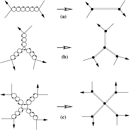
where () are the generators of the flavor SU(n) in the matrices, and the currents () are singlets of the U(N) family symmetry. The summation over flavor and family indices has been entirely suppressed in the kinetic energy and mass term. While this Lagrangian is symmetric under the global SU(n)U(N) symmetry, it is obviously not invariant under gauge rotations of SU(n) or U(N) on . When the coupling constant is positive and larger than some critical value, the interaction generates vector bound states of a family singlet that form the adjoint representation of the flavor SU(n). In the leading order, explicit computation of the infinite fermion chain in Fig. 1 allows us to obtain for the bound states not only the mass and the coupling to the fermions but also the triple and quartic self-couplingsSuzuki . Although quadratic divergence does not appear in the loop diagrams thanks to global current conservation, logarithmic divergences do. We regularize them by the dimensional regularization. The result is remarkable: All the couplings of the composite vector bosons obey SU(n) gauge invariance. The effective Lagrangian written in terms of and reads in the standard notation
| (2) |
where denotes the SU(n) adjoint vector fields in an matrix and . The gauge coupling constant and the boson mass are obtained from the loop diagram as
| (3) |
where in the dimensional regularization. It is only the mass term of the composite vector-boson fields that is not gauge invariant in the effective Lagrangian of Eq. (2). Furthermore, the four-fermion interactions of the original Lagrangian of the constituent fermions disappear from , i.e., nonrenormalizability of the current-current interaction is also transferred entirely into this composite boson mass term.
The composite boson mass squared can be made as small as one likes by increasing the magnitude of the coupling of binding , but it can never reach zero for any finite value of . This is because each loop of the fermion self-energy chain is of the transverse form with by the global current conservation of SU(n) symmetry and consequently iteration of the loops leads to the fermion-antifermion scattering amplitude of the form,
| (4) | |||||
Since with near , the location of the bound-state pole determined by is at . Notice the importance of in order to have . This cannot be realized without global SU(n) current conservation. For bound states other than spin-parity , the natural scale of mass squared is or else ( = momentum cutoff). Furthermore we should appreciate that the same global current conservation prevents us from bringing the vector bound-state pole to . This is consistent with the general theoremCase by Case-Gasiorowicz and Weinberg-Witten that asserts incompatibility of the charged massless vector bosons with the Lorentz-covariant conserved currents carrying nonvanishing charges. Putting it more simply, a massless spin-one boson cannot be obtained in the continuous limit of a massive spin-one boson, as we all know. If we took literally the limit of , the mass would become zero, i.e., the composite bosons would look like gauge bosons. In this limit the entire Lagrangian would become alone after rescaling of the fields and therefore trivially gauge invariant. However, the global currents would not exist by the Noether theorem in this pathological gauge-invariant limit. Conflict with the theorem could be thus evaded, but this limit is a case of no interest, physically or mathematically.
How can these gauge-invariant couplings be generated ? It is easy to understand when one works in the functional integral methodGeorgi ; Bando . The partition function in terms of the fields is given in the Euclidean metric by
| (5) |
We can replace the current-current interaction by introducing the auxiliary adjoint vector fields as
| (6) |
where the added Lagrangian term is defined in the Minkowski metric by
| (7) |
Summation over the flavor is understood above and in the following. Equivalence of the two actions in Eqs. (5) and (6) is obvious since one can trivially integrate out the fields in Eq. (6) after shifting in the functional space. When we open up and add it to , the current-current interactions cancel out between and , leaving the effective Lagrangian in the Minkowski metric in the form of
| (8) | |||||
The constant in front of should be identified with the gauge coupling so that
| (9) |
The functional integration over in Eq. (6) is equivalent to rewriting the current-current interaction with the exchange at zero-momentum transfer. This explains the relation in Eq. (9) as . While the diagram calculation has determined and individually as given in Eq. (3), the mass in Eq. (8) is still a free parameter. The reason is that we have not yet incorporated the dynamical information of the fermion loop at this stage of the functional integral formulation.
The Lagrangian has no kinetic energy term of so that its equation of motion for reads
| (10) |
It simply means that, before letting the vector-bosons propagate, they are made of fermion-antifermion pairs. The global current conservation assures that the composite fields consist only of spin-one states by leaving out the O(3) scalar component at this stage.

We can now proceed to generate the kinetic energy term and the self-couplings of dimension four for from the loop diagrams. With of Eq. (8), iteration of the fermion loops no longer occurs for the two-point function of since there is no four-fermion interaction left in . The relevant diagrams are only the single fermion-loop diagrams of in the leading order of . [Fig. 2(a)]. The same is true for the three and four-point functions. We should notice here that is gauge invariant up to the mass term of since the interaction can be combined with the fermion kinetic energy term into the gauge-invariant form;
| (11) |
The painstaking diagram calculationSuzuki for the two, three and four-point functions of was actually unnecessary; they must come out in the gauge-invariant combination up to the overall constant since the sole term of gauge noninvariance, namely, the vector-meson mass term , does not enter the loop calculation in the leading order. Therefore the radiatively produced Lagrangian of dimension four for the fields ought to be in the form
| (12) |
An explicit loop-diagram calculation is needed only to obtain the constant . The fermion loop of Fig. 2a gives
| (13) |
The constant is absorbed into the wave-function renormalization of by , which in turn renormalizes the coupling and the vector-boson mass too;
| (14) |
Because of there is no additive mass renormalization when the mass is computed at zero momentum. After the kinetic energy term of is computed and the renormalization of Eq. (14) is performed, the renormalized coupling is given by
| (15) |
and the mass takes the form of
| (16) | |||||
These agree with the results of the loop-diagram iteration, Eq. (3). Namely, the values for and that were obtained in the calculation of the infinite chain of loops actually incorporate the renormalization of Eq. (14). The complete effective Lagrangian written in , , and thus takes the SU(n) gauge-invariant form up to the boson mass term as given in Eq. (2) with the understanding that the renormalization of Eq. (14) has already been done for the mass and the coupling.
Before moving on, we summarize this section: In the explicitly solvable model of fermionic constituents a set of composite spin-one bosons behave exactly like gauge bosons in the small limit of the composite boson mass even though the fundamental Lagrangian is explicitly gauge noninvariant. Gauge noninvariance stays but solely in the mass term of the composite bosons. Since the origin of the boson mass is not spontaneous breaking of gauge symmetry, there is no asymmetric vacuum condensate of a scalar field, elementary nor composite. A hidden symmetry can be introduced in the fermionic model of the Nambu-Jona-Lasinio type, if one wishes, by using its language, but it is always broken in this case. There is no unbroken phase of the hidden symmetry except for the pathological limit of Bando .
We have chosen the four-fermion binding force here in order to demonstrate all solutions explicitly in the cutoff field theory. Rather than going into a discussion of phenomenological relevance, we explore in the succeeding sections whether this remarkable phenomenon of dynamical gauge-symmetry generation is realized in other models or not, specifically, in the case that the constituents are spinless bosons. The option of bosons being fundamental particles is even more esoteric phenomenologically and sounds less attractive. Our purpose here is, however, to obtain a better understanding of this generation mechanism of an approximate gauge symmetry from other models.
III Case of bosonic constituents: abelian symmetry
We would like to see whether the gauge-symmetry generation of the preceding section works in the bosonic constituent models or not. We emphasize that we do not slip an unbroken local symmetry in our models to look for massless vector bosons as dynamical gauge boson modes. Such a study was done in the a few decades ago; a local symmetry is present at the beginning as redundancy when its Lagrangian is written in some form, then a composite massless vector boson is searched for. Instead we choose models in which there is no local symmetry to start with. We study whether the explicit breaking can be transformed into the mass term alone in the case of tightly bound vector bosons. Unlike the fermionic model, to our knowledge, our bosonic models have never been studied in the literature. They show us more clearly what realizes an approximate gauge symmetry as a consequence of compositeness.
Let us first study the case of an Abelian vector boson since it gives us a good insight into the problem leaving out unnecessary complications. We form a neutral composite vector boson (a massive photon) with charged spinless bosons like having heavy mass . We introduce families of the heavy for the large expansion. Our fundamental Lagrangian is written in the nonpolynomial form as
| (17) |
with the charged spinless bosons and () of families. No constraint is imposed on the fields and the classical vacuum is at so that the Lagrangian is invariant under the global U(1) charge rotation,
| (18) |
and trivially invariant under global U(N) family rotations. The current-current interaction has been so chosen that not only a tightly bound state can be formed but also its mass is explicitly calculable in the large limit.111It may look that the factor of in this Lagrangian has some vague resemblance with that of the model written in the constrained fieldsHaber . But our are unconstrained here.
A natural extension of the fermionic model might suggest the current-current interaction of in the bosonic case. However, this simple current-current interaction does not generate a tightly bound vector boson in the scattering amplitude for the following reasons:
1. The current , is not a conserved current in the case that the interaction is . Because derivatives of enter , the conserved current222 Hereafter we denote the Noether currents with the capital letters and distinguish them from the naive bosonic currents that originates from the kinetic energy term alone. derivable by the Noether theorem in the Abelian case,
| (19) |
contains a term which depends on the interaction . If we went ahead with this naive current-current interaction , the current would not conserve, . Its immediate consequence is that the self-energy loop is not transverse () and an additional term of quadratic divergence arises with the coefficient . This moves the pole to that cannot be physically interpreted as mass square of a bound state.
2. From the standpoint of the functional formalism, choosing the simple interaction would amount to postulating that the composite vector field be proportional to and consequently lead to . That is, would not be purely a field of spin-one, but contain a spin-zero component.
We were fortunate in the model of fermionic constituents since the binding interaction contains no derivative of fields and therefore the choice of the interaction was deceptively simple. In contrast, for the bosonic constituents we must choose the interaction carefully such that the auxiliary composite field is proportional to the Noether current. If so chosen, the field obeys and its proper self-energy part turns out to be transverse. Only in this situation can the composite boson mass be made as small as one likes by increasing the binding interaction constant . The factor in the denominator of the interaction in Eq. (17) serves this purpose and realizes . [See the second relation in Eq. (3).]
III.1 Diagram computation
A neutral vector bound-state is formed with the loop and bubble diagrams of . We compute for the bound-state in elastic scattering
| (20) |
Although we are interested in physics at large , we cannot make the expansion in the Lagrangian since the potential term behaves at large as
| (21) |
The behavior of at makes the perturbative vacuum ill-defined and prevents diagram calculation. We must instead perform diagram calculation in the perturbative expansion in powers of to all orders, sum up the perturbative series and then take to large values. Such computation is possible only in the leading order. In the large limit the relevant diagrams are chains of loops with bubbles added. (See Fig. 3.) Each loop comes from the diagram of , while the bubble diagram arise from in the power series expansion of the factor . If the loops and the bubbles of in the channel sum into the transverse form as
| (22) |
the perturbation series turns into the total scattering amplitude in the form of Eq. (4) so that the bound-state mass comes out to be . Transversality of Eq. (22) is indeed realized after summing the loops and the bubbles of the same order in the power of , as shown in Fig. 3. In the tree diagram is the only diagram [Fig. 3(a)]. A single-loop diagram and a single-bubble diagram enter [Fig. 3(b)]. The single-loop diagram alone would not make transverse in , as we know from the photon self-energy in electrodynamics of the charged pions in which the bubble generated by the interaction makes the photon self-energy transverse and keeps the photon massless even after loop corrections. In we sum a diagram with two bubbles, a pair of diagrams with one-loop and one-bubble, and the diagram of two bubbles [Fig. 3(c)]. We can keep on going to higher orders of and obtain a scattering amplitude of the form of Eq. (22) in the channel. Consequently, the location of the pole is found at as we desire. In order to realize this behavior, therefore, the factor is needed in the interaction term of the Lagrangian, Eq. (17).

When we sum up an infinite series of the loop plus bubble diagrams of Fig. 3 in a compact form, the resulting invariant amplitude for the elastic scattering of Eq. (20) is
| (23) | |||||
where
| (24) |
The bound-state pole appears in at the location determined by . For large the mass of the bound state is found at
| (25) |
and its coupling to is given by
| (26) |
so that the bound-state mass and the coupling are related at by
| (27) |
Here again the composite mass vanishes if one takes the limit of in Eq. (25). Going back to the original Lagrangian, Eq. (17), we find in this limit333This limiting Lagrangian appeared in Reference Akh in a different context.
| (28) |
It is not difficult to check that this Lagrangian is U(1)-gauge invariant under . The U(1)-gauge invariance is nontrivial in this form unlike that in the fermionic model. In the nonlinear representation, however, this limiting Lagrangian turns out to be the free Lagrangian of the radial fields and the phase fields do not enter. That is, this Lagrangian is trivially gauge invariant and of little physical content. The Noether current of Eq. (19) vanishes
| (29) |
Since there is not a conserved global U(1) current, the massless limit of our composite boson would not contradict the general theoremCase . But it is obvious that a massless vector boson cannot be formed with the limiting Lagrangian that contains only the Hermitian radial field.
The Lagrangian of Eq. (28) would be identical to that of the model if were constrained with . However, the fields are the unconstrained fields in our case; we have gone through the Feynman diagram calculation with the standard (unconstrained) spinless-boson propagator.
III.2 Functional integral formulation
In the diagram computation above, we need careful bookkeeping in summing up the perturbation series into the scattering amplitude. After our study of the fermionic model, however, we are able to carry out an equivalent calculation by the functional integral method in a simpler way. We see underlying issues and their new aspects more clearly in a new light.
The first step is to introduce the auxiliary neutral vector field . The Lagrangian of Eq. (17) in suggests the form for the partition function,
| (30) |
where is given by Eq. (17) and is defined by
| (31) | |||||
Upon integration over , the factor in front of the first term of Eq. (31) generates , as is shown in the Appendix, and cancels the last term of so that Eq. (30) reduces to the partition function written in alone,
| (32) |
The diagrammatic content of this logarithmic term is also shown in the Appendix. The infinite factor represents the total functional phase space , which should be properly regularized. Physically, it is a large finite number since the unrenormalizable Lagrangian of Eq. (17) is valid only up to some limited energy range. However, if one regularizes it dimensionally as the limit of
| (33) |
one would set this to zero using the formula
| (34) |
Containing no derivative, the term is manifestly gauge invariant by itself and, in the leading order, does not contribute to the calculation of the bound state in the channel. It affects only the channel of scattering in the leading order. We leave this singular term as proportional to as it is, while it does not affect our diagrammatic calculation in the rest of the paper.
When we sum and , no current-current interaction is left in the sum,
| (35) | |||||
In fact, we have chosen in Eq. (31) so that the current-current interaction is absent from the sum in Eq. (35). We have not obtained Eq. (35) by simply gauging with in Eq. (17). We identify the constant in front of with the gauge coupling in Eq. (35). Therefore we obtain , which is the relation between and that has been obtained in Eq. (27) by the diagram calculation. Furthermore a new four-point interaction of arises in ,
| (36) |
which is equal to thanks to . Therefore the Lagrangian in Eq. (35) can be rearranged into the gauge-invariant form up to the mass term of :
| (37) | |||||
The Lagrangian of Eq. (37) leads to the equation of motion for ,
| (38) |
The Noether current in terms of and can be computed with Eq. (19) from as
| (39) |
Therefore, the equation of motion, Eq. (38), together with says that, with our choice of Lagrangian, is proportional to the Noether current of the constituent fields before propagation;
| (40) |
Consequently it satisfies so that its self-energy is transverse. Therefore, the bound-state mass square can behave as . The relation also tells that this vector boson is not a gauge boson since it holds by the equation of motion, not by choice of fixing ambiguities. Nor does transform like under either. That is, we are studying something very different from the gauge boson of the modelHaber or its hidden symmetryBando .
We now proceed to obtain the kinetic energy term through loop diagrams. No three-point function or nonderivative four-point function of is generated in the Abelian case. It is only the two-point functions that arise from loop and bubble diagrams. The computation is straightforward by the diagrams of Fig. 4 with the interaction .

Since the interaction added with is gauge invariant and since the mass term of enters nowhere in this loop and bubble calculation, the resulting kinetic energy is also gauge invariant:
| (41) |
where the constant is computed with the loop diagram from the Lagrangian of Eq. (37);
| (42) |
This constant is removed by the wave-function renormalization of the field and renormalization of the coupling , and the mass :
| (43) |
The renormalized mass and coupling are what the diagram computation has given in Eqs. (25) and (26) as in the fermionic model. Even after they are renormalized, they maintain the relation of Eq. (27). We have thus confirmed the results of our preceding diagram calculation in the bosonic model and have reaffirmed our finding in the fermionic model: In the small limit of the composite boson mass the bosonic theory also approaches the gauge theory as closely as possible although the mass can never be brought to zero for any large but finite value of .
We have a little deeper understanding of the relation between gauge invariance and the small composite boson mass in the bosonic constituent model than in the fermionic model. In the case of the bosonic constituents we must be very careful in choosing the binding interaction; the composite boson mass approaches zero in the limit of strong coupling if we multiply the naive current-current interaction with the factor . This factor conspires with and generates part of the gauge interaction with the correct strength when we move to the effective theory in terms of the composite field . The equation of motion for prior to generation of the kinetic energy is of the form,
| (44) |
where the right-hand side is proportional to the Noether current. Expanding the denominator in the power series of , we interpret the series as the composite vector boson consisting not only of a single pair of in wave but also of many additional pairs in wave. Even with this additional factor , the original Lagrangian written in the fields is not gauge invariant at all. After we introduce the composite vector field , however, gauge noninvariance is swept entirely into its mass term and we reach the correct form of the gauge boson Lagrangian (up to mass).
Before we proceed to the non-Abelian case, we summarize what we have learned from the models that we have so far studied.
1. In order to generate composite vector bosons with small mass, their proper self-energy part must be of the transverse form without an additional term ( since this transverse form guarantees that the composite mass square is inversely proportional to strength of binding interaction.
This transversality is realized in our models with the conserved currents of a global symmetry. For this reason, presence of a global symmetry is a prerequisite for a generation of (approximate) gauge symmetry though it may not be surprising. If conserved currents of a global symmetry do not exist, the composite boson mass cannot be made small. By turning the argument around, we may say that if a tightly bound state of exists, there must be some dynamical reason why such tight binding occurs. Without a good reason the bound-state mass would only be some fraction of . In the channel a very strong current-current interaction of right properties can generate a tightly bound state of mass scale much lower than , at least theoretically, as we have seen above.
2. Keeping this observation in mind, we should set up a model Lagrangian possessing a global symmetry and introduce nonpropagating composite vector-boson fields that are proportional to the Noether currents. Then the resulting Lagrangian of the composite fields is gauge invariant except for the mass term. When the Lagrangian is written in the constituent particle fields alone, gauge symmetry does not exist since it is broken by their kinetic energy and, in the case of boson constituents, by the binding interaction too. However, after composite vector bosons are generated dynamically, the gauge symmetry breaking is entirely absorbed into the boson mass term.
IV Case of bosonic constituents: Nonabelian symmetry
After we have gone through the functional integral formulation of the Abelian model, it is not difficult to extend the results to the non-Abelian case. We choose here the bosonic constituents that transform like the fundamental representation under flavor SU(n) symmetry. The bosonic fields that carry flavors are replicated with families as (). As we have learned in the Abelian case, the simplest current-current interaction summed over flavors does not serve our purpose since are not conserved currents in the presence of the bosonic current-current interaction. We need the non-Abelian version of the factor ] given in Eq. (17). The right factor in the non-Abelian case is an matrix in the flavor space. It is expressed as the inverse matrix of
| (45) |
where are the -dimensional representation matrices of SU(n). The matrix is symmetric in the of flavors and independent of families. In the special case of SU(2), turns out to be a diagonal matrix in flavors thanks to . For notational simplicity, we suppress hereafter the family indices and often even flavor indices when they are obvious. Our Lagrangian is chosen as
| (46) |
where summation is understood over flavors () in the interaction term, and are the “naive” currents defined by
| (47) |
The flavor and family indices are suppressed altogether in the kinetic energy and mass terms. Between the currents and is the element of the inverse matrix of , not the inverse of . This is the right current-current interaction that generates tightly bound vector-boson states of SU(n).
The Noether currents of SU(n) can be computed with Eq. (46) by using the non-Abelian version of Eq. (19) as
| (48) |
Being the Noether currents, satisfy the conservation law, . By choosing the auxiliary composite fields proportional to the Noether currents , we implement . In order to accomplish it, we add to as
| (49) |
where
| (50) |
The determinant of here means the determinant in the flavor SU(n) space. It compensates the same term of the opposite sign that arises upon the functional integration in the partition function,
| (51) |
so that is equal to what we have before introducing the fields . Just as in the Abelian case, the logarithmic term does not contribute to our calculation of bound states in the leading order.
Let us examine the Lagrangian of Eq. (49). Opening up the mass term of and adding it to , we find the simple form,
| (52) | |||||
where the flavor indices have been suppressed; the term in the last term stands for . The current-current interaction in is cancelled out by the term arising from in .
The coefficient of is identified with the gauge coupling in Eq. (52);
| (53) |
With this relation in mind, we can write the part of the term in Eq. (52) explicitly in the form
| (54) |
Therefore the three terms, , , and , add up in the gauge-invariant kinetic energy term;
| (55) |
The remaining task is to generate the kinetic energy term of . We compute the non-Abelian counterpart of the loop and the bubble in Fig.4 for the two-point function and, in addition, the three-point and four-point functions in the leading order. Since is gauge-invariant up to the mass of and no composite boson loop enters in the leading order, this calculation inevitably generates the gauge-invariant combination of , and as
| (56) |
where is the covariant field tensors in matrix,
| (57) |
Since we know that the final result should come out to be proportional to , we have only to compute one of its terms, say, the two-point function. We find through an explicit diagram calculation
| (58) |
As before, the constant is renormalized away by
| (59) |
Therefore the final Lagrangian is
| (60) | |||||
where it is understood that renormalization has been made for and as in Eq. (59). This completes our derivation in the non-Abelian case. Clever use of the functional integral method streamlines the whole derivation and greatly alleviates the calculation that would be quite cumbersome in the diagrammatic method.
A final remark is again on distinction of our study from the model. In the strong coupling limit of at which the composite boson mass goes to zero, the nonabelian Lagrangian in terms of approaches the form
| (61) |
where . It has no resemblance to the model in any respect. In this limit the composite bosons of SU(n) turn massless and the Lagrangian becomes gauge invariant under the flavor SU(n). The Noether currents, Eq. (48), vanish at so that there is no conflict with the no-go theoremCase . However, it is questionable whether such “gauge bosons” have any physical significance or even exist at all. (See the remark made on this limit in the Abelian case.) As for the large expansion, our large is the number of families not of flavors while it is the number of our flavors that is made large in the computation of the model.
V Extended model of fermionic constituents
The condition of tight binding imposes strong constraints on the binding interaction. In fact, it determines the form of interaction almost uniquely. After we have gone through our models, we are able to extend the original fermionic model a little by adding the force proportional to to the force. Let us discuss briefly such a model of abelian symmetry. We study the Lagrangian defined by
| (62) | |||||
where
| (63) |
Summation over families () is understood in , and , while the flavor of is a simple Abelian charge. In Eq. (62) is a free dimensionless parameter that determines the amount of -wave mixing. The value of must be positive in order for the well-defined vacuum to exist. The interaction has been so chosen that the Noether current comes out in a reasonably simple form:
| (64) |
Although the term has been introduced to generate the force with the same order in strength as the force, the current enters the Noether current by one power higher in than the current since arises from the kinetic energy term too. Following the procedure in the previous models, we introduce the auxiliary field with the Lagrangian term
| (65) | |||||
where
| (66) |
The Lagrangian leads to the equation of motion for ,
| (67) |
The field obeys and the proper self-energy part is transverse. Adding to , we have
| (68) | |||||
where . Note that the field enters precisely in the gauge-invariant form up to the mass term. Therefore, upon generating the kinetic energy of by loops and bubbles and renormalizing away by , and , we reach in terms of the renormalized mass and coupling
| (69) | |||||
where , . The four-fermion interaction does not go away in Eq. (69) but gauged with . The sole gauge-noninvariant term is the mass term . Although it looks tempting to introduce another auxiliary vector field to remove the “gauged term” from the Lagrangian of Eq. (69), it is not possible since the coefficient of is positive (repulsive).444Positivity of is required by existence of a well-defined classical vacuum. For the denominator would blow up at in Eq. (62).
Since the four-fermion interaction stays in the Lagrangian , the wave-function renormalization and therefore the mass and the coupling are to be computed in the perturbation series with respect to . We rewrite in terms of and by use of and carry out the computation. In the zeroth order of the simple one-loop-diagram of fermion is transverse by itself and generates . In the first order of there exist four diagrams which sum up to the transverse form. (See. Fig. 5.) When we compute divergent integrals by the dimensional regularization, we find that the correction to happens to vanish by cancellation among the four diagrams.

In the order of there are again four diagrams, which differ from the diagrams of by insertion of a single fermion loop . This insertion maintains the cancellation that occurs among the four diagrams of . The same cancellation repeats to all higher orders of . Consequently we have no correction to :
| (70) |
to all orders of in the large expansion. Therefore the renormalized mass and coupling are given by and . Absence of the correction is unexpected. We are unable to appreciate if it has an important implication or not.
This extended fermionic model reinforces the claim that the generation mechanism of approximate gauge symmetry is not an accident but more a general phenomenon. As we have emphasized repeatedly, however, it would be a futile effort to try to improve the Lagrangian further so as to generate genuine gauge bosons of zero mass as composite states unless some local symmetry is slipped in. It is because it would contradict with the simple general theoremCase . In our case the Lorentz-covariant conserved currents with nonzero charge do exist in the composite vector-boson theories as we can write them in terms of the constituent particle fields. We have shown for each model in this paper that the conserved (Noether) currents would disappear and the fundamental Lagrangian would become meaningless when one took the massless limit. In the extended fermion model the Noether current would disappear and the Lagrangian would become singular at .
VI Discussion and outlook
Gauge symmetries in particle physics are broken symmetries except for electrodynamics and chromodynamics. The prevailing wisdom for broken gauge symmetries is that they are spontaneously broken since otherwise the underlying quantum field theory would be unrenormalizable. If we want to construct an ultimate fundamental theory valid at all possible energies from top down, postulating gauge symmetry is the only option for us. On the other hand there may still be layers of effective theories before we reach the ultimate theory at the highest energy. Indeed this was the case in the history of phenomenological particle physics. If one takes this viewpoint, one may rather build particle theory from the bottom up with effective theories which are valid only over limited ranges of the energy scale. It would not be so unreasonable for theorists in this camp to ask whether there is any dynamical origin for approximate gauge symmetries other than spontaneous symmetry breaking.
The purpose of this paper is to show in the solvable models that even if a gauge symmetry is not implanted at a fundamental level, it may emerge as an approximate symmetry by dynamical necessity in the tightly bound limit of composite vector bosons if such bosons exist at all. We know that the Nambu-Goldstone boson can be a tightly bound composite massless boson: It appears upon spontaneous breaking of a global symmetry and a phase transition occuring. In our case a global symmetry remains unbroken and no phase transition occurs. The tightly bound composite boson is not unnatural in the channel when the composite field is proportional to a Lorentz-covariant conserved current. In contrast, in other channels one must fine-tune coupling strength if one wants to generate a very light but nonzero composite boson. We have postulated a global symmetry as our starting point to derive an approximate local symmetry. Some may ask why we accept a global symmetry at the beginning. Are global symmetries more natural than local symmetries ? Frankly, we cannot make a convincing argument in this regard.
In low-energy strong interactions of mesons and baryons the relation between vector mesons and conserved hadronic currents was emphasized by SakuraiSakurai nearly a half century ago. He strongly advocated that the , the , and the meson couple to the isospin, the baryonic, and the hypercharge current, respectively, in the form incorporating the mixing. A decade later, from a field theory standpoint, Kroll, Lee and ZuminoLee proposed the field-current identity hypothesis in which the fields of the , the and the meson are in fact the isospin, the baryon and the hypercharge current themselves. Our finding in this paper reminds us of this old hypothesis although in the contemporary picture those light vector mesons are the loosely bound states by the long-distance confining forces. Nonetheless, these hypotheses on the light vector mesons were successfully tested, for instance, in the vector-meson dominance of the electromagnetic and weak currents albeit within the accuracy of typical low-energy strong interaction physics. Many years later, but before high-energy electroweak interaction data were accumulated, Claudson, Farhi and Jaffe Jaffe proposed that and might be loosely bound composite bosons by some hypothetical confining force. Criticism was made by Lee and Shrock Shrock with lattice gauge theory analysis. Beyond that, however, conspicuously missing was a quantitative study. The idea of the loosely bound and would have hard time to withstand test of the contemporary experimental data with respect to the fast falling form-factor damping, e.g., large difference between the on-shell coupling and the zero-momentum limit of coupling. More recently, however, attempts have been made for composite and with higher confinement energy scales involving the extra space-time dimensionGher . The guage symmetry is placed at onset outside the four-dimensional spacetime in those models.
Our field theory models here are all based on unrenormalizable field theories in the large limit since otherwise we cannot solve them explicitly. When the models are written in the effective Lagrangian of the composite vector bosons, unrenormalizability is transformed into the longitudinal polarization of the massive vector bosons and, in the presence of derivative interactions, possibly the nonderivative gauge-invariant logarithmic term. In this sense our ignorance in the binding interactions is swept into the longitudinal polarization state of the composite vector-boson. As it is well knownQuigg , the tree diagrams involving the self-coupling of longitudinal polarizations of the and bosons overshoot the unitarity bound at energies much higher than the and masses when the Higgs boson is left out or very heavy ( 1 TeV) in the standard model. A possibility of building an alternative to the standard model with composite and was suggestedGeorgi by introducing a set of sufficiently many new fermions as their consituents in our simplest fermionic model. In such models and would interact strongly at very high energies through the longitudinal polarization modes. This alone does not rule out the composite and at present. However, there exists a potential problem of the same origin at lower energies. That is, the radiative corrections to the low-energy electroweak parameters. We can examine the composite vector-boson propagator with the diagram of Fig. 1a by taking the external fermion lines off mass shell. It is given by
| (71) |
where the form factor is defined with by
| (72) |
so that is normalized as . The function does not deviate much from that of the lowest-order perturbation in the region of .555 The damping effect of is measured by its radius defined by where . In our fermionic model , which is as we expect. Since models of composite and do not contain the Higgs bosons, the mass singularity term potentially generates large radiative corrections666 It was argued years agoR that for some four-fermion interaction theory may become renormalizable when it is written in terms of collective modes, i.e., composite fields. It does not seem to happen in our case of vector bosons. to the low-energy parameters, particularly in the parameter. However, the diagrams which contain a composite boson loop are in the next-to-leading order of the large expansion. That is, it is technically outside of our scope of calculation. Nonetheless it may become a problem if we seriously attempt to build a model of composite and as an alternative to the standard model.
We all agree that despite its field theoretical beauty the standard model has disturbing unnaturalness, the worst of it being the hierarchy problem, once we go beyond the multi-TeV energy scale. We should not completely abandon esoteric possibilities such as composite and at some very high energy-scale until an experiment rules them out convincingly. We should keep our mind open for the outcome of the upcoming accelerator experiment although admittedly chances may be small. Even if the LHC does not support the composite and bosons, it may discover novel spin-one bosons that interact like gauge bosons. Aside from an experiment, the quest for the origin of gauge symmetry will remain a challenge for many theoristsNielsen .
Acknowledgements.
The author acknowledges useful conversations with Korkut Bardakci. This work was supported by the Director, Office of Science, Office of High Energy and Nuclear Physics, Division of High Energy Physics, of the U.S. Department of Energy under Contract No. DE–AC02–05CH11231.Appendix A The functional determinant
Change of the integral variable from to in the functional integral of Eq. (30) is not so trivial as that in the ordinary integrals. Although the resulting logarithmic term does not contribute to the final results of our particular computation, a remark should be made in order to assure that this change of variable does not generate a new gauge-symmetry breaking.
We go to the Euclidean metric by and and examine the functional integral
| (73) |
where . We may drop the tilde of by shifting the functional space of by . The factor may also be dropped since the rescaling of by a constant affects only an unphysical constant factor to the partition function. However, the multiplication of a function on cannot be dropped in general since it deforms the functional phase space. For notational simplicity, we study for one of the four space-time components of suppressing its subscript for a while. The integral of our interest is therefore:
| (74) |
where . Expand in a complete set of orthonormal functions () in the 4-dimensional space-time as
| (75) |
where . The functional integral Eq. (74) turns into
| (76) |
where . If we choose specifically the complete set with which the matrix is diagonal, the integral can be carried out with the quadrature integral formula as
| (77) | |||||
Since is the determinant of the infinite-dimensional diagonal matrix , the last line of Eq. (77) can be expressed as
| (78) |
where we have supplied the superscript to in order to emphasize that is a diagonal matrix. The undetermined (infinite) multiplicative constant in front of the exponent is absorbed into the ill-defined measure of functional phase space that has no physical effect.
Going back to Eq. (77), let us expand the logarithm with the Taylor series expansion formula of as
| (79) | |||||
Note that for the diagonal matrix, and furthermore that a trace of the matrix element does not depend on the choice of its basis. Therefore, we can go to the four-dimensional Fourier basis () and rewrite Eq. (79) as
| (80) | |||||
where the last factor comes from
| (81) |
In the diagram calculation the function arises from the quartic divergence of the -bubble diagram, as will be shown later in this Appendix. Putting back in Eq. (74), we reach
| (82) | |||||
| (83) |
where the four space-time components of generate four identical
terms to turn into in
the right-hand side of Eq. (82). The irrelevant constant
in front has been suppressed above.
Diagrammatic explanation
In the remainder of Appendix we show the diagrammatic origin of this logarithmic term. Let us expand both sides of Eq. (82) in the power series of and compare order by order the right-hand side with their corresponding diagrams computed with of Eq. (37) in the left-hand side. Our purpose here is pedagogical; We show that the integration over generates Green’s functions from pairs of and indeed leads to the logarithmic term in Eq. (82). The vector-boson two-point function for the Lagrangian of Eq. (37) is given by
| (84) |
since there is no kinetic energy term of at this stage.
The term of in the right-hand side is . This arises from the diagram Fig. 6a that consists of a single Green’s function of :
| (85) | |||||
This term is the quartically divergent self-energy of , but cancelled out in the final answer by the one-loop self-energy diagram of the interaction .
When we move to the order and higher, there exist the contributions of connected and disconnected diagrams. The terms of in the expansion of the right-hand side of Eq. (82) are
| (86) |
where means square of the term of in Eq. (85), that is, the disconnected diagram of two bubbles (the first diagram of Fig. 6b). The first term of Eq. (86) comes from the connected diagram in Fig. 6b:
| (87) | |||||
| (88) |
where the first factor 2 comes from two different ways of matching fields into two-point functions and is from the second-order perturbation expansion. Summation over subscripts and generates the factor of 4 in the last line. This agrees with the term of Eq. (82) in the expansion. The term proportional to
| (89) |
appears from the disconnected diagrams in the left-hand side and matches the second-order Taylor expansion of the term in the right-hand side of Eq. (82).

We can go on to and higher-order terms. The term in the exponent of the right-hand side is , while the connected diagrams of in the left-hand side matches this term:
| (90) |
where the factor comes from the third-order perturbation expansion, the factor in front is due to eight ways to pair ’s into two-point Green’s functions, the factor 4 in front of results from the sum over the polarization subscript of , and each comes from a Green’s function of . The disconnected terms match in much the same way as in the case of .
References
-
(1)
W. Heisenberg, Rev. Mod. Phys. 29, 269 (1957).
H. P. Dürr, Heisenberg, H. Mitter, S. Schlieder, and K. Yamazaki, Z. Naturforsh. 14A, 441 (1959).
J. D. Bjorken, Ann. Phys. (N.Y.) 24, 174 (1963).
I. Bialynicki-Birula, Phys. Rev. 130, 465 (1963).
T. Eguchi and H. Sugawara, Phys. Rev. D 10, 4257 (1974); T. Eguchi, Phys. Rev. D 14, 2755 (1976).
K. Kikkawa, Progr. Theor. Phys. 56, 947 (1976).
Y. Terazawa, Y. Chikashige, and K. Akama, Phys. Rev D 15, 480 (1977); K. Akama, Phys. Rev. Lett. 76, 184 (1996); K. Akama and T. Hattori, Phys. Lett. B 393, 383 (1997).
-
(2)
C. D. Froggatt and H. B. Nielsen, Origin of Symmetries
(World Scientific, Singapore, 1991) and references therein.
J. L. Chikaleuli, C. D. Froggatt, and H. B. Nielsen, Phys. Rev. Lett. 87 091601 (2001). -
(3)
M. Veltman, Acta Phys. Pol. B12, 437 (1981).
S. Mandelstam, A Passion in Physics edited by C. DeTar et al. (World Scientific, Singapore, 1985), p.97. - (4) M. Suzuki, Phys. Rev. D 37, 210 (1988).
- (5) J. D. Bjorken, Phys. Rev. D 19, 335 (1979).
- (6) P. Q. Hung and J. J. Sakurai, Nucl. Phys. bf B143, 81 (1978); 148B, 538(E) (1979).
- (7) A. Cohen, H. Georgi, and E. Simmons, Phys. Rev. D 38, 405 (1988).
- (8) M. Bando, T. Kugo, and K. Yamawaki, Phys. Rep. 164, 217 (1988).
-
(9)
K. M. Case and S. Gasiorowicz, Phys. Rev. 125, 1055 (1962).
S. Weinberg and E. Witten, Phys. Lett. 96B, 59 (1980). - (10) H. E. Haber, I. Hinchliffe, and E. Rabinovici, Nucl. Phys. B 172, 458 (1980).
- (11) E. K. Akhmedov, Phys. lett. B521, 79 (2001).
- (12) J. J. Sakurai, Ann. Phys. (N.Y.) 11, 1 (1960).
- (13) N. M. Kroll, T. D. Lee, and B. Zumino, Phys. Rev. 157, 1376 (1967); T. D. Lee and B. Zumino, Phys. Rev. D 163, 1667 (1967).
-
(14)
M. Claudson, E. Farhi, and R. L. Jaffe, Phys. Rev. D 34, 873 (1986).
- (15) I-H. Lee and R. E. Shrock, Phys. Rev. Lett. 59, 14 (1987); Phys. Lett. 199B, 541 (1987); Phys. Lett. 201B, 497 (1988); S. Aoki, I-H. Lee, and R. E. Shrock, Phys. Lett. 207B, 471 (1988).
- (16) For instance, Y. Cui, T. Gherghetta, and J. D. Wells, J High Energy Phys. 09 (2009) 080 and references therein.
- (17) B. W. Lee, C. Quigg, and H. Thacker, Phys. Rev. Lett. 38, 883 (1977); Phys. Rev. D 16, 1519 (1977).
-
(18)
See J. D. Bjorken, in [1].
I Bialynicki-Birula, Phys. Rev. 130, 465 (1963).
G. S. Guralnik, Phys. Rev. 136, B1404 (1964).
T. Eguchi, Phys. Rev. D 17, 611 (1978).