A Gram Determinant for Lickorish’s Bilinear Form

Abstract

We use the Jones-Wenzl idempotents to construct a basis of the Temperley-Lieb algebra $TL_{n}$. This allows a short calculation for a Gram determinant of Lickorish’s bilinear form on the Temperley-Lieb algebra.

Keywords: Skein Theory, Temperley-Lieb Algebra.

1 Introduction

In [W], Witten proposed the existence of 3-manifold invariants. A mathematically rigorous definition was given by Reshetikhin and Turaev [RT] using quantum groups and Kirby calculus [K]. Later, Lickorish [L1] provided an alternative proof by using a bilinear form on the Temperley-Lieb algebra $TL_{n}$. An important property Lickorish needed was that this bilinear form defined over $\mathbb{Z}[A,A^{-1}]$ is degenerate at certain $4(n+1)$th roots of unity and nondegenerate at $4i$th roots of unity for $i<n+1$. Ko and Smolinsky obtained this result by using a recursive formula for the determinants of specific minors of this form [KS]. They did not give a closed form for the determinant. This was first done by Di Francesco, Golinelli and Guitter [FGG]. Di Francesco later gave a simpler proof. In this paper, we give a short derivation by using a skein-theoretic approach together with a combinatorial proposition from Di Francesco [F]. In order to do this, we construct a nice basis $\mathfrak{D}_{n}$ for $TL_{n}$. In fact, there have been several bases of $TL_{n}$ studied before. See [FGG], [F], or [GS]. It turns out that $\mathfrak{D}_{n}$ is a rescaled version of the basis used in [F], but the properties of Jones-Wenzl idempotents significantly simplify the calculation. Our skein-theoretic approach is motivated by the colored graph basis for TQFT modules developed in Blanchet, Habegger, Masbaum, Vogel’s paper [BHMV]. A skein theoretic derivation of a Gram determinant for the type B Temperley-Lieb algebra is given in [CP].

2 Temperley-Lieb Algebra

Let $F$ be an oriented surface with a finite collection of points specified in its boundary $\partial F$. A link diagram in the surface $F$ consists of finitely many arcs and closed curves in $F$, with a finite number of transverse crossings, each assigned over or under information. The endpoints of the arcs must be the specified points in $\partial F$. We define the skein of $F$ as follows:

Definition 2.1.

Suppose $A$ is a variable. Let $\Lambda$ be the ring $\mathbb{Z}[A,A^{-1}]$ localized by inverting the multiplicative set generated by elements of $\{A^{n}-1\mid n\in\mathbb{Z}^{+}\}$. The linear skein $\mathcal{S}(F)$ is the module of formal linear sums over $\Lambda$ of link diagrams in $F$ quotiented by the submodule generated by the skein relations:

1. $L\cup U=\delta L$, where $U$ is a trivial knot, $L$ is a link in $F$ and $\delta=(-A^{-2}-A^{2})$;

2. $\begin{minipage}{14.45377pt}\includegraphics[width=14.45377pt]{skein1.pdf}\end{minipage}=\ A^{-1}\ \begin{minipage}{14.45377pt}\includegraphics[width=14.45377pt]{skein2.pdf}\end{minipage}\ +\ A\ \begin{minipage}{14.45377pt}\includegraphics[width=14.45377pt]{skein3.pdf}\end{minipage}$ .

Now, taking $F$ to be the 2-disk $D^{2}=I\times I$, we have:

Definition 2.2.

The $n^{th}$ Temperley-Lieb Algebra $TL_{n}$ is the linear skein $\mathcal{S}(D^{2},n)$, where $n$ means there are $n$ points specified in $I\times\{0\}$ and $I\times\{1\}$ respectively.

It is well known that $TL_{n}$ has a basis, which consisting of non-crossing figures. We denote this basis by $\mathfrak{B}_{n}$. Some special elements $\{1,e_{1},...,e_{n-1}\}$ of the basis are shown in Figure 1. As an algebra, $TL_{n}$ is generated by those special elements.

$$1=\begin{array}[]{c}\includegraphics[width=72.26999pt,height=86.72377pt]{1.pdf}\end{array}e_{i}=\begin{array}[]{c}\includegraphics[width=72.26999pt,height=86.72377pt]{e_i.pdf}\end{array}$$

Figure 1: The integer $i$ beside the arc means $i$ parallel copies of the arc.

A significant property of this algebra in quantum invariant theory is that there is a natural bilinear form on $TL_{n}$. In [L1], Lickorish used this form to construct quantum invariants of 3-manifolds. We construct this bilinear form with respect to the basis $\mathfrak{B}_{n}$ that we gave above:

Definition 2.3.

Define a map on $\mathfrak{B}_{n}\times\mathfrak{B}_{n}$ to $\Lambda$ as follows:

$G_{n}(s,r)=\begin{minipage}{14.45377pt}\includegraphics[width=14.45377pt]{leftbracket.pdf}\end{minipage}\begin{minipage}{72.26999pt}\includegraphics[width=72.26999pt]{map.pdf}\end{minipage}\begin{minipage}{14.45377pt}\includegraphics[width=14.45377pt]{rightbracket.pdf}\end{minipage}$ ,

where $s=\begin{minipage}{21.68121pt}\includegraphics[width=21.68121pt]{A.pdf}\end{minipage}$ and $r=\begin{minipage}{21.68121pt}\includegraphics[width=21.68121pt]{B.pdf}\end{minipage}$ are elements in $\mathfrak{B}_{n}$ and $<,>$ is the Kauffman bracket. We extend this map to a bilinear form on $TL_{n}$, and still denote it by $G_{n}$. We denote the determinant of $G_{n}$ with respect to $\mathfrak{B}_{n}$ by $\det(G_{n})$.

In this paper, we give a simple proof of the determinant of this bilinear form with respect to the basis $\mathfrak{B}_{n}$, which was also proved in [FGG]. The following is the main result.

Theorem 2.4.

$$\det(G_{n})=\Delta_{1}^{c_{n}}\prod_{k=1}^{n}(\frac{\Delta_{k}}{\Delta_{k-1}})^{\alpha_{k}}$$

where $\Delta_{i}=\frac{(-1)^{i}(A^{2(i+1)}-A^{-2(i+1)})}{A^{2}-A^{-2}}$, $c_{n}=\frac{1}{n+1}\left(\begin{array}[]{c}2n\\ n\end{array}\right)$, and $\alpha_{k}=\left(\begin{array}[]{c}2n\\ n-k\end{array}\right)-\left(\begin{array}[]{c}2n\\ n-k-1\end{array}\right).$

Remark 2.5.

From now on, we will use $\operatorname{card}$ to denote the cardinality of a set and $\det$ the determinant of a matrix.

3 Properties of $TL_{n}$

In the 1990’s, the properties of $TL_{n}$ were studied by Lickorish [L2], Masbaum-Vogel [MV], Kauffman-Lins [KL] and some other people. Below we will summarize some results on $TL_{n}$ that we will be using.

In this algebra, there is a sequence of idempotents, which are very important in constructing 3-manifold invariants. We will mainly use these idempotents to construct a basis for $TL_{n}$. They are defined as follows:

Proposition 3.1.

There is a unique element $f_{n}\in TL_{n}$, called $n^{th}$ Jones-Wenzl idempotent, such that

1. $f_{n}e_{i}=0=e_{i}f_{n}$ for $1\leq i\leq n-1$;

2. $(f_{n}-1)$ belongs to the subalgebra generated by $e_{1},...,e_{n-1}$;

3. $f_{n}f_{n}=f_{n}$.

Remark 3.2.

We can put a box on the segment to denote the idempotent. But we will abbreviate the box from now on. Hence, we put an $n$ beside the string to denote $n$ parallel strings with an idempotent inserted, if otherwise is not stated. For example, we denote the figure on the left in Figure 2 by the figure on the right, which will be used frequently in this paper.

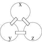
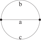
Figure 2: The left figure lies in $S^{2}$. The right figure is an abbreviation of the left one, where $a=x+y,b=y+z,c=x+z$. We denote the value of this diagram in $\mathcal{S}(S^{2})$by $\Theta(a,b,c)$.

For the next property, we first set up some notation. Consider the skein space of the disc $D$ with $a+b+c$ specified points on its boundary. The points are partitioned into three sets of $a,b,c$ consecutive points. The effect of adding the idempotents $f_{a},f_{b},f_{c}$ just outside every diagram in such a disc with specified points is to map the skein space of the disc into a subspace of itself. We denote this subspace by $T_{a,b,c}$.

Definition 3.3.

The triple $(a,b,c)$ of nonnegative integers will be called admissible if $a+b+c$ is even, $a\leq b+c$ and $b\leq c+a$ and $c\leq a+b$.

Proposition 3.4.

$$dim(T_{a,b,c})=\left\{\begin{array}[]{l l}0&\quad\text{if $a,b,c$ are not admissible};\\ 1&\quad\text{if $a,b,c$ are admissible}.\\ \end{array}\right.$$

When $(a,b,c)$ is admissible, $T_{a,b,c}$ has a generator $g$ on the left in Figure 3. We usually denote it in a simple way by the diagram on the right in the figure.

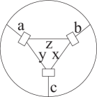
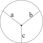
Figure 3: On the left is the generator of $T_{a,b,c}$. On the right is an abbreviation of the generator.

Proposition 3.5.

$$\begin{minipage}{72.26999pt}\includegraphics[width=72.26999pt]{O.pdf}\end{minipage}=\frac{\delta_{ad}\Theta(a,b,c)}{\Delta_{a}}\ \begin{minipage}{72.26999pt}\includegraphics[width=72.26999pt]{f_a.pdf}\end{minipage}\ ,$$

where $\delta_{ad}$ is the Kronecker delta.

Similarly, consider the skein space of the disc $D$ with $a+b+c+d$ specified points on its boundary. The points are partitioned into four sets of $a,b,c,d$ consecutive points. The effect of adding the idempotents $f_{a},f_{b},f_{c},f_{d}$ just outside every diagram in such a disc with specified points is to map the skein space of the disc into a subspace of itself. We denote this subspace by $Q_{a,b,c,d}$.

Proposition 3.6.

A base for $Q_{a,b,c,d}$ is the set of elements as in Figure 4, where $j$ takes all values for which both $(a,b,j)$ and $(c,d,j)$ are admissible.

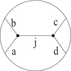
Figure 4: A basis element of $Q_{a,b,c,d}$

Proposition 3.7.

$$\begin{minipage}{72.26999pt}\includegraphics[width=72.26999pt]{f_af_b.pdf}\end{minipage}=\sum\frac{\Delta_{j}}{\Theta(a,b,j)}\ \begin{minipage}{72.26999pt}\includegraphics[width=72.26999pt]{Q2.pdf}\end{minipage}$$

where the summation runs over all $j$’s such that $(a,b,j)$ is admissible.

Remark 3.8.

We denote $\frac{\Theta(a,b,1)}{\Delta_{a}}$ by $\Gamma(b,a)$. It is easy to see that $\Gamma(b,a)=0$ if $\|a-b\|>1$. Then Proposition 3.5 becomes

$$\begin{minipage}{72.26999pt}\includegraphics[width=72.26999pt]{NewO.pdf}\end{minipage}=\delta_{ad}\Gamma(b,a)\ \begin{minipage}{72.26999pt}\includegraphics[width=72.26999pt]{f_a.pdf}\end{minipage}\ .$$

4 A Basis for the Temperley-Lieb Algebra from Jones-Wenzl Idempotents

Several bases of $TL_{n}$ have been given before by, for example, [FGG] and [GS]. The idea of constructing the basis in this paper is motivated by [BHMV] and [L3]. They constructed bases for modules associated to surfaces by a certain topological quantum field theory. These bases were indexed by coloring of a trivalent graph in a handlebody.

Definition 4.1.

Let $D_{a_{1},...,a_{2n-1}}$ be the element of $TL_{n}$ in the Figure 5 where $a_{i}$ satisfies:

1. $a_{1}=a_{2n-1}=1$;

2. $a_{i}\in\mathbb{N}$ for all $i$;

3. $\|a_{i}-a_{i-1}\|=1$ for all $i$.

Let $\mathfrak{A}_{n}$ be the collection of all n-tuples $(a_{1},...,a_{2n-1})$ satisfying the above conditions, and let $\mathfrak{D}_{n}$ be the collection of all these $D$’s.

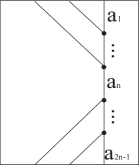
Figure 5: Each triple point is admissible.

Lemma 4.2.

Suppose $(a_{1},...,a_{2n-1})$ and $(b_{1},...,b_{2n-1})$ satisfy all conditions above except $a_{1}=a_{2n-1}=1$. Then

$$\langle D_{a_{1},...,a_{2n-1}},D_{b_{1},...,b_{2n-1}}\rangle$$

$$= \delta_{a_{1}b_{1}}...\delta_{a_{2n-1}b_{2n-1}}\Gamma(a_{1},a_{2})\Gamma(a_{2},a_{3})\dots\Gamma(a_{2n-2},a_{2n-1})\Delta_{a_{2n-1}}\ .$$

Proof.

We prove the formula by induction.
When $n=2$, by direct computation,

$$\langle D_{a_{1},a_{2},a_{3}},D_{b_{1},b_{2},b_{3}}\rangle$$

$$= \delta_{a_{1}b_{1}}\Gamma(a_{1},a_{2})\delta_{a_{2}b_{2}}\Gamma(a_{2},a_{3})\delta_{a_{3}b_{3}}\Delta_{a_{3}}.$$

Thus the formula is true for $n=2$. Now suppose the formula is true for $n=k-1$ and let $n=k$.

$$\langle D_{a_{1},...,a_{2n-1}},D_{b_{1},...,b_{2n-1}}\rangle$$

$$= \delta_{a_{1}b_{1}}\Gamma(a_{1},a_{2})\delta_{a_{2n-1}b_{2n-1}}\Gamma(a_{2n-2},a_{2n-1})\langle D_{a_{2},...,a_{2n-2}},D_{b_{2},...,b_{2n-2}}\rangle$$

$$= \delta_{a_{1}b_{1}}\Gamma(a_{1},a_{2})\delta_{a_{2n-1}b_{2n-1}}\Gamma(a_{2n-2},a_{2n-1})\times$$

$$\delta_{a_{2}b_{2}}...\delta_{a_{2n-2}b_{2n-2}}\Gamma(a_{2},a_{3})\Gamma(a_{3},a_{4})\Gamma(a_{2n-3},a_{2n-2})\Delta_{a_{2n-2}}$$

$$= \delta_{a_{1}b_{1}}...\delta_{a_{2n-1}b_{2n-1}}\Gamma(a_{1},a_{2})\Gamma(a_{2},a_{3})\dots\Gamma(a_{2n-2},a_{2n-1})\Delta_{a_{2n-1}}.$$

Thus the formula holds for $n=k$. Hence, by induction, the formula holds. ∎

Lemma 4.3.

The elements of $\{D_{a_{1},...,a_{2n-1}}\}$ are orthogonal in $TL_{n}$, and so are linearly independent.

Proof.

This follows from Lemma 4.2. ∎

Now, we are going to prove that the elements of $\mathfrak{D}_{n}$ generate $TL_{n}$. This can be proved using induction and Proposition 3.1 and 3.4. For variety, we give an alternative proof.

Lemma 4.4.

Each element of $\{1,e_{1},...,e_{n-1}\}$ can be expressed as a linear combination of $D$’s in $\mathfrak{D}_{n}$.

Proof.

We prove the lemma by induction and Proposition 3.7.
It is easy to see that the lemma is true for $\mathfrak{D}_{1},\mathfrak{D}_{2}$.
Suppose the lemma is true for $\mathfrak{D}_{n-1}$, we need show that it is true for $\mathfrak{D}_{n}$.
For $x\in\{1,e_{2},e_{3},...,e_{n-1}\}$, we can obtain the result as in Figure 6. The proof for $e_{1}$ is similar except at the second equality, we use Proposition 3.7 for each turn-back, see Figure 7. ∎

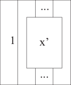
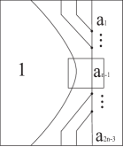
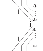
Figure 6: $x^{\prime}s$ is a generator for $TL_{n-1}$ by deleting the first arc in $x$. The first equality is from induction step. The second equality is from Proposition 3.7.

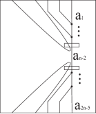
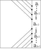
Figure 7: The proof is the same as in Figure 6 except we need use Proposition 3.7 twice.

Lemma 4.5.

$\mathfrak{D}_{n}$ is a basis of $TL_{n}$.

Proof.

Since each element in $\mathfrak{B}_{n}$ can be written as a product of $e_{i}$’s, we can write each as a sum of products of elements in $\mathfrak{D}_{n}$ by Lemma 4.4. Moreover, a product of elements in $\mathfrak{D}_{n}$ can be written as a linear combination of elements in $\mathfrak{D}_{n}$ by Proposition 3.5. So we can write elements in $\mathfrak{B}_{n}$ as sums of elements in $\mathfrak{D}_{n}$. As $\mathfrak{B}_{n}$ is a basis for $TL_{n}$, the lemma holds. ∎

5 Relation between $\mathfrak{B}_{n}$ and $\mathfrak{D}_{n}$

In this section, we will give a new system to denote the basis $\mathfrak{B}_{n}$. We draw a diagram similar to elements in $\mathfrak{D}_{n}$ as in Figure 8, except we do not put idempotents on strings and we put an empty circle at each black triple point. If $a_{i}=a_{i+1}+1$, we put Figure 10 in the corresponding circle. If $a_{i}=a_{i+1}-1$, then we put Figure 10 in the corresponding circle. After filling all circles, we get a non-crossing diagram in $TL_{n}$ for each sequence $(a_{1},...,a_{2n-1})$, which satisfies the conditions in Definition 4.1. Those elements belong to $\mathfrak{B}_{n}$. Now, we give a total order on the set $\mathfrak{A}_{n}$ as follows: $(a_{1},...,a_{2n-1})<(b_{1},...,b_{2n-1})$ if there is a $j$ such that $a_{i}=b_{i}$ for all $i<j$ and $a_{j}<b_{j}$. This order on $\mathfrak{A}_{n}$ induces an order on $\{B_{a_{1},...,a_{2n-1}}\}$ and $\mathfrak{D}_{n}$ naturally. In this order, we will show that the representing matrix of $\{B_{a_{1},...,a_{2n-1}}\}$ with respect to basis $\mathfrak{D}_{n}$ is upper triangular having $1$’s on the diagonal.

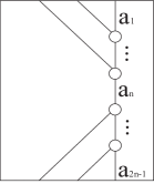
Figure 8: An example of $B_{a_{1},...,a_{2n-1}}$.

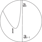
Figure 9: $a_{i}=a_{i+1}+1$

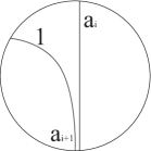
Figure 10: $a_{i}=a_{i+1}-1$

Lemma 5.1.

$\langle B_{a_{1},a_{2},...,a_{2n-1}},D_{b_{1},b_{2},...,b_{2n-1}}\rangle=0$ if $(a_{1},a_{2},...,a_{2n-1})<(b_{1},b_{2},...,b_{2n-1})$.

Proof.

Since $(a_{1},a_{2},...,a_{2n-1})<(b_{1},b_{2},...,b_{2n-1})$, there is a $j$ such that $a_{j}<b_{j}$. If we pair $B_{a_{1},a_{2},...,a_{2n-1}}$ and $D_{b_{1},b_{2},...,b_{2n-1}}$ together, we can find a circle passing through them at $a_{j}$ and $b_{j}$. We cut the pairing along this circle to get an element as in Figure 11. By the properties of idempotents, it is easy to see that this element is 0 in $\mathcal{S}(D^{2})$ with $a_{j}$ and $b_{j}$ on the boundary. So we get the result. ∎

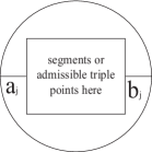
Figure 11: We have the idempotent at $b_{j}$ and no idempotent at $a_{j}$.

Before we go on, we introduce a lemma and a corollary.

Lemma 5.2.

$\Theta(n,n+1,1)=\Delta_{n+1}$, and $\Theta(n,n-1,1)=\Delta_{n}$.

Proof.

$$\Theta(n,n+1,1)$$

$$= \begin{minipage}{72.26999pt}\includegraphics[width=72.26999pt]{Theta1.pdf}\end{minipage}=\begin{minipage}{72.26999pt}\includegraphics[width=72.26999pt]{Theta2.pdf}\end{minipage}$$

$$= \begin{minipage}{72.26999pt}\includegraphics[width=72.26999pt]{Theta3.pdf}\end{minipage}=\begin{minipage}{72.26999pt}\includegraphics[width=72.26999pt]{Theta4.pdf}\end{minipage}$$

$$= \Delta_{n+1}$$

Similarly, it is easy to see that $\Theta(n,n-1,1)=\Delta_{n}$. ∎

Corollary 5.3.

$$\Gamma(b,a)=\begin{cases}1&\text{if $a=b+1$,}\\ \frac{\Delta_{a+1}}{\Delta_{a}}&\text{if $a=b-1$.}\par\end{cases}$$

Proof.

This follows easily from Lemma 5.2. ∎

Now, we can prove the following:

Proposition 5.4.

$\langle B_{a_{1},a_{2},...,a_{2n-1}},D_{a_{1},a_{2},...,a_{2n-1}}\rangle\ =\ \langle D_{a_{1},a_{2},...,a_{2n-1}},D_{a_{1},a_{2},...,a_{2n-1}}\rangle$ for all ${(a_{1},a_{2},...,a_{2n-1})}$ in $\mathfrak{A}_{n}$.

Proof.

We prove this by induction on $n$. Suppose $n=2$. Then it is easy to check that

$$\langle B_{1,0,1},D_{1,0,1}\rangle\ =\ \langle D_{1,0,1},D_{1,0,1}\rangle,\langle B_{1,2,1},D_{1,2,1}\rangle\ =\ \langle D_{1,2,1},D_{1,2,1}\rangle.$$

Assume that the result is true for $n<k$. We will prove it is true for $n=k$. For $(a_{1},...,a_{2n-1})=(1,2,...,k,...,2,1)$, we have

$$\langle B_{1,2,...,k,...,2,1},D_{1,2,...,k,...,2,1}\rangle\ =\ \langle D_{1,2,...,k,...,2,1},D_{1,2,...,k,...,2,1}\rangle$$

by direct computation. For $(a_{1},...,a_{2n-1})\neq(1,2,...,k,...,2,1)$, we choose $i>k>j$ such that $a_{i-1}=a_{i+1}$, $a_{j-1}=a_{j+1}$ and $a_{i}=a_{i-1}+1$, $a_{j}=a_{j-1}+1$. Then by Proposition 3.5, we have

$$\langle B_{a_{1},a_{2},...,a_{2n-1}},D_{a_{1},a_{2},...,a_{2n-1}}\rangle$$

$$= \Gamma(a_{i},a_{i+1})\Gamma(a_{j},a_{j+1})$$

$$\times\langle B_{a_{1},...,\hat{a}_{i},\hat{a}_{i+1},...\hat{a}_{j},\hat{a}_{j+1},...,a_{2n-1}},D_{a_{1},...,\hat{a}_{i},\hat{a}_{i+1},...,\hat{a}_{j},\hat{a}_{j+1},...,a_{2n-1}}\rangle$$

where the hat on $a_{i}$ means that it is removed.
It is easy to see that

$$B_{a_{1},...,\hat{a}_{i},\hat{a}_{i+1},...\hat{a}_{j},\hat{a}_{j+1},...,a_{2n-1}}\in\mathfrak{B}_{n-2},D_{a_{1},...,\hat{a}_{i},\hat{a}_{i+1},...,\hat{a}_{j},\hat{a}_{j+1},...,a_{2n-1}}\in\mathfrak{D}_{n-2}.$$

By Lemma 4.2 and Corollary 5.3,

$$\langle D_{a_{1},a_{2},...,a_{2n-1}},D_{a_{1},a_{2},...,a_{2n-1}}\rangle$$

$$= \Gamma(a_{i},a_{i+1})\Gamma(a_{j},a_{j+1})$$

$$\times\langle D_{a_{1},...,\hat{a}_{i},\hat{a}_{i+1},...\hat{a}_{j},\hat{a}_{j+1},...,a_{2n-1}},D_{a_{1},...,\hat{a}_{i},\hat{a}_{i+1},...,\hat{a}_{j},\hat{a}_{j+1},...,a_{2n-1}}\rangle.$$

By induction,

$$\langle B_{a_{1},...,\hat{a}_{i},\hat{a}_{i+1},...\hat{a}_{j},\hat{a}_{j+1},...,a_{2n-1}},D_{a_{1},...,\hat{a}_{i},\hat{a}_{i+1},...,\hat{a}_{j},\hat{a}_{j+1},...,a_{2n-1}}\rangle$$

$$= \langle D_{a_{1},...,\hat{a}_{i},\hat{a}_{i+1},...\hat{a}_{j},\hat{a}_{j+1},...,a_{2n-1}},D_{a_{1},...,\hat{a}_{i},\hat{a}_{i+1},...,\hat{a}_{j},\hat{a}_{j+1},...,a_{2n-1}}\rangle.$$

Hence,

$$\langle B_{a_{1},a_{2},...,a_{2n-1}},D_{a_{1},a_{2},...,a_{2n-1}}\rangle=\langle D_{a_{1},a_{2},...,a_{2n-1}},D_{a_{1},a_{2},...,a_{2n-1}}\rangle.$$

∎

Proposition 5.5.

$$\begin{pmatrix}B_{1,2,...,n,...,1}\\ \vdots\\ B_{1,0,1,0,...,0,1}\end{pmatrix}=\begin{pmatrix}1&*&\cdots&*\\ 0&1&\cdots&*\\ \vdots&\vdots&\ddots&\vdots\\ 0&0&\cdots&1\end{pmatrix}\begin{pmatrix}D_{1,2,...,n,...,1}\\ \vdots\\ D_{1,0,1,0,...,0,1}\end{pmatrix}.$$

Proof.

This follows easily from Lemma 5.1 and Proposition 5.4. ∎

Corollary 5.6.

$\{B_{a_{1},...,a_{2n-1}}\}=\mathfrak{B}_{n}$.

Proof.

By Proposition 5.5, we can see that $B_{a_{1},...,a_{2n-1}}\neq B_{b_{1},...,b_{2n-1}}$ if $(a_{1},...,a_{2n-1})\neq(b_{1},...,b_{2n-1})$. Moreover, $\operatorname{card}\{B_{a_{1},...,a_{2n-1}}\}=\operatorname{card}\mathfrak{D}_{n}=\operatorname{card}\mathfrak{B}_{n}$ and $\{B_{a_{1},...,a_{2n-1}}\}\subset\mathfrak{B}_{n}$. So we have $\{B_{a_{1},...,a_{2n-1}}\}=\mathfrak{B}_{n}$. ∎

By Corollary 5.6 and linear algebra, we can see that the $\det(G_{n})$ we get by using the basis $\mathfrak{B}_{n}$ is the same as $\det(G_{n})$ we get by using the basis $\mathfrak{D}_{n}$.

6 Lattice path

Definition 6.1.

A lattice path in the plane is a path from $(0,0)$ to $(a,b)$ with northeast and southeast unit steps, where $a,b\in\mathbb{Z}$. A Dyck path is a lattice path that never goes below the $x-$axis. We denote the set of all Dyck path from $(0,0)$ to $(a,b)$ by $\mathcal{D}_{(a,b)}$.

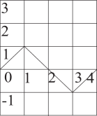
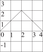
Figure 12: On the left is a lattice path. On the right is a Dyck path.

Remark 6.2.

There is a natural bijection $f$ from $\mathfrak{D}_{n}$ to $\mathcal{D}_{(2n,0)}$, the set of all Dyck paths from $(0,0)$ to $(2n,0)$ as follows:
For each $D_{a_{1},...,a_{2n-1}}\in\mathfrak{D}_{n}$, we construct a path from $(0,0)$ to $(2n,0)$ with step $(i,a_{i})$ for all $1\leq i\leq 2n-1$. Since $a_{i}$ satisfies

1. $a_{1}=a_{2n-1}=1$;

2. $a_{i}\in\mathbb{N}$ for all $i$;

3. $\|a_{i}-a_{i-1}\|=1$ for all $i$.

We can see that this is a Dyck path.

Remark 6.3.

The reflection principle [C, page 22] says that the number of all Dyck paths from $(0,0)$ to $(2n,0)$ is the Catalan number $C_{n}=\frac{1}{n+1}\binom{2n}{n}$. Hence, we recover the well-known result that the dimension of $TL_{n}$ is $C_{n}$.

7 Proof of the Main Theorem

Now we can start our proof of the main theorem. By Lemma 4.3, we know that $\{D_{a_{1},...,a_{2n-1}}\}$ is an orthogonal basis with respect to the bilinear form. Thus the matrix of $G_{n}$ is a diagonal matrix under this basis. We have

$$\det(G_{n})=\prod_{(a_{1},...,a_{2n-1})}\langle D_{a_{1},...,a_{2n-1}},D_{a_{1},...,a_{2n-1}}\rangle.$$

Then by Lemma 4.2, we have

$$\det(G_{n})=\prod_{(a_{1},...,a_{2n-1})}\Gamma(a_{1},a_{2})\Gamma(a_{2},a_{3})\dots\Gamma(a_{2n-2},a_{2n-1})\Delta_{1}.$$

Using Lemma 5.3, we can simplify $\det(G_{n})$ as follows:
Consider the tuple $(D,i)$ such that $D$ is an element of $\mathfrak{D}_{n}$ and $a_{i}=k$ in $D$. If $a_{i+1}=k+1$, then $\Gamma(a_{i},a_{i+1})$ is 1 by Lemma 5.3. So $(D,i)$ will contribute 1 to $\det(G_{n})$. If $a_{i+1}=k-1$, then $\Gamma(a_{i},a_{i+1})=\frac{\Delta_{k+1}}{\Delta_{k}}$. So $(D,i)$ will contribute $\frac{\Delta_{k}}{\Delta_{k-1}}$ to $\det(G_{n})$. We denote by $\mathfrak{S}_{k}$ the set of all tuple $\{(D,i)\}$ with $D\in\mathfrak{D}_{n}$ and $a_{i}=k,a_{i+1}=k-1$ in $D$. Let $\alpha_{k}$ be the cardinality of $\mathfrak{S}_{k}$. Then

$$\det(G_{n})=\Delta_{1}^{\operatorname{card}\mathfrak{D}_{n}}\prod_{k=1}^{n}(\frac{\Delta_{k}}{\Delta_{k-1}})^{\alpha_{k}}\ .$$

Now, the theorem is reduced to calculate $\alpha_{k}$ for each $k$.

Proposition 7.1.

$$\alpha_{k}=\left(\begin{array}[]{c}2n\\ n-k\end{array}\right)-\left(\begin{array}[]{c}2n\\ n-k-1\end{array}\right).$$

Proof.

In Section 6, we already had a 1-1 correspondence $f$ between $\mathfrak{D}_{n}$ (the new basis we constructed) and $\mathcal{D}_{(2n,0)}$ (Dyck paths from $(0,0)$ to $(2n,0)$). With respect to this correspondence, each pair $(D,i)$ in $\mathfrak{S}_{k}$ is associated to a pair $(f(D),i)$ with $a_{i}=k,a_{i+1}=k-1$ in $f(D)$, that is the step from $(i,a_{i}=k)$ to $(i+1,a_{i+1}=k-1)$ in the path $f(D)$. See Figure 13 for an example. Denote by $\mathcal{S}_{k}$ the set of all pairs $(f(D),i)$, where $f(D)$ has a step from $k$ to $k-1$ at $i$. Thus we have a 1-1 correspondence between $\mathfrak{S}_{k}$ and $\mathcal{S}_{k}$.

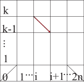
Figure 13: The bold step is a step going down from $(i,a_{i}=k)$ to $(i+1,a_{i+1}=k-1)$.

Di Francesco [F, page 562] set up a 1-1 correspondence from $\mathcal{S}_{k}$ to $\mathcal{D}_{(2n,2k)}$. Then we have

$$\alpha_{k}=\operatorname{card}{\mathcal{D}_{(2n,2k)}}=\left(\begin{array}[]{c}2n\\ n-k\end{array}\right)-\left(\begin{array}[]{c}2n\\ n-k-1\end{array}\right).$$

For the convenience of reader, we now give Di Francesco’s correspondence in our terminology. For an element $\hat{P}\in\mathcal{D}_{(2n,2k)}$, it should intersect the horizontal line $y=k$ in a point $p=(i,a_{i}=k)$ with $a_{i+1}=k+1$ and $a_{i-1}=k-1$ at least once. Let $p$ be the rightmost such intersection. Now we cut $\hat{P}$ at the point $p$, reflect the right part of $\hat{P}$ with respect to $y$-axis, and shift it down by $k$ units. Then we glue this part back to the left part. We get a Dyck path $P$ from $(0,0)$ to $(2n,0)$. In the resulting path $P$, we then choose the smallest $i^{\prime}\geq i$, such that $a^{\prime}_{i}=k$ and $a_{i^{\prime}+1}=k-1$. We associate the path $\hat{P}$ to the pair $(P,i^{\prime})$. Therefore, we construct a map $\phi:\mathcal{D}_{(2n,2k)}\rightarrow\mathcal{S}_{k}$.
Conversely, for a pair $(P,i)$, where $P\in\mathcal{D}_{(2n,0)}$. We choose the largest $i^{\prime}\leq i$ with $a_{i^{\prime}}=k$ and $a_{i^{\prime}-1}=k-1$. We cut the path $P$ at $i^{\prime}$, reflect the right part with respect to the $y$-axis, shift up by $n$ units and glue it back. Thus we construct a path $\hat{P}$ in $\mathcal{D}_{(2n,2k)}$. We associate the tuple $(P,i)$ to the path $\hat{P}$. Therefore, we construct a map $\varphi:\mathcal{S}_{k}\rightarrow\mathcal{D}_{(2n,2k)}$.
It is easy to see that $\phi\varphi=id$ and $\varphi\phi=id$. Therefore, we have constructed a 1-1 correspondence between $\mathcal{S}_{k}$ and $\mathcal{D}_{(2n,2k)}$.

By the reflection principle, we have

$$\operatorname{card}\mathcal{D}_{(2n,2k)}=\left(\begin{array}[]{c}2n\\ n-k\end{array}\right)-\left(\begin{array}[]{c}2n\\ n-k-1\end{array}\right).$$

Therefore, we have

$$\alpha_{k}=\left(\begin{array}[]{c}2n\\ n-k\end{array}\right)-\left(\begin{array}[]{c}2n\\ n-k-1\end{array}\right).$$

∎

8 Relation between $\mathfrak{D}_{n}$ and Di Francesco’s second basis.

In this section, we extend our ring $\Lambda$ to the complex numbers $\mathbb{C}$ and let $A$ be any non-zero complex number which is not a root of unity.

Definition 8.1.

$$ND_{a_{1},...,a_{2n-1}}=\frac{D_{a_{1},...,a_{2n-1}}}{<D_{a_{1},...,a_{2n-1}},D_{a_{1},...,a_{2n-1}}>^{\frac{1}{2}}}.$$

We call $ND_{a_{1},...,a_{2n-1}}$ the normalization of $D_{a_{1},...,a_{2n-1}}$, and denote the normalized basis by $\mathfrak{ND}_{n}$.

Theorem 8.2.

$\mathfrak{ND}_{n}$ is the same basis as Di Francesco’s second basis in [F].

Proof.

Di Francesco defined his orthonormal basis by a recursive equation [F, equation 3.19, Page 555]. So we just need to show that $\mathfrak{ND}_{n}$ satisfies the recursive equation and the initial condition.

Let $D_{a_{1},...,a_{i-1},a_{i},a_{i+1},...,a_{2n-1}}$ and $D_{a_{1},...,a_{i-1},a^{\prime}_{i},a_{i+1},...,a_{2n-1}}$ be two elements in $\mathfrak{D}_{n}$ such that $a_{i}=a_{i-1}-1=a_{i+1}-1$ and $a^{\prime}_{i}=a_{i}+2$, that means they are equal everywhere except at $i$th arc. Then using the recursive formula for Jones-Wenzl idempotents at $i$th arc, we have

$$D_{a_{1},...,a_{i-1},a_{i^{\prime}},a_{i+1},...,a_{2n-1}}=D_{a_{1},...,a_{i-1},\hat{a}_{i},a_{i+1},...,a_{2n-1}}-\frac{\Delta_{a_{i}}}{\Delta_{a_{i}+1}}D_{a_{1},...,a_{i-1},a_{i},a_{i+1},...,a_{2n-1}}$$

where $D_{a_{1},...,a_{i-1},\hat{a}_{i},a_{i+1},...,a_{2n-1}}$ is as in Figure 14.

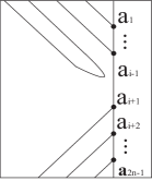
Figure 14: $a_{i}$ disappears.

Since $a_{i-1}=a_{i+1}$, this is well defined. It is easy to see that $D_{a_{1},...,a_{i-1},\hat{a}_{i},a_{i+1},...,a_{2n-1}}=e_{i}D_{a_{1},...,a_{i-1},a_{i},a_{i+1},...,a_{2n-1}}$, where $e_{i}$ acts on $D_{a_{1},...,a_{i-1},a_{i},a_{i+1},...,a_{2n-1}}$ as in [F]. We divide the equation by the norm of $D_{a_{1},...,a_{i-1},a_{i^{\prime}},a_{i+1},...,a_{2n-1}}$ on both sides. By Lemma 4.2, we have

$$ND_{a_{1},...,a_{i-1},a^{\prime}_{i},a_{i+1},...,a_{2n-1}}$$

$$= \frac{(e_{i}D_{a_{1},...,a_{i-1},a_{i},a_{i+1},...,a_{2n-1}}-\frac{\Delta_{a_{i}}}{\Delta_{a_{i}+1}}D_{a_{1},...,a_{i-1},a_{i},a_{i+1},...,a_{2n-1}})}{(\Gamma(a_{1},a_{2})\dots\Gamma(a_{i-1},a^{\prime}_{i})\Gamma(a^{\prime}_{i},a_{i+1})\dots\Gamma(a_{2n-2},a_{2n-1})\Delta_{a_{2n-1}})^{\frac{1}{2}}}$$

$$= (e_{i}-\frac{\Delta_{a_{i}}}{\Delta_{a_{i}+1}})ND_{a_{1},...,a_{i-1},a_{i},a_{i+1},...,a_{2n-1}}\times$$

$$\frac{(\Gamma(a_{1},a_{2})\dots\Gamma(a_{i-1},a_{i})\Gamma(a_{i},a_{i+1})\dots\Gamma(a_{2n-2},a_{2n-1})\Delta_{a_{2n-1}})^{\frac{1}{2}}}{(\Gamma(a_{1},a_{2})\dots\Gamma(a_{i-1},a^{\prime}_{i})\Gamma(a^{\prime}_{i},a_{i+1})\dots\Gamma(a_{2n-2},a_{2n-1})\Delta_{a_{2n-1}})^{\frac{1}{2}}}$$

$$= (e_{i}-\frac{\Delta_{a_{i}}}{\Delta_{a_{i}+1}})ND_{a_{1},...,a_{i-1},a_{i},a_{i+1},...,a_{2n-1}}\frac{(\Gamma(a_{i-1},a_{i})\Gamma(a_{i},a_{i+1}))^{\frac{1}{2}}}{(\Gamma(a_{i-1},a^{\prime}_{i})\Gamma(a^{\prime}_{i},a_{i+1}))^{\frac{1}{2}}}$$

$$= (e_{i}-\frac{\Delta_{a_{i}}}{\Delta_{a_{i}+1}})ND_{a_{1},...,a_{i-1},a_{i},a_{i+1},...,a_{2n-1}}\frac{(\Gamma(a_{i-1},a_{i}))^{\frac{1}{2}}}{(\Gamma(a^{\prime}_{i},a_{i+1}))^{\frac{1}{2}}}\ .$$

By definition,

$$\Gamma(a_{i-1},a_{i})=\mu_{a_{i}},\Gamma(a^{\prime}_{i},a_{i+1})=\mu_{a_{i+1}},$$

where $\mu_{i}$ as in [F]. Thus, $\mathfrak{ND}_{n}$ satisfies the recursive equation. Moreover, it is easy to see that

$$u_{n}=ND_{1,0,1,0,...,0,1,0,1},$$

where $u_{n}$ is as in [F, equation 3.5,Page 551]. So $\mathfrak{ND}_{n}$ satisfies the initial condition. ∎

References

- [BHMV] Blanchet, C.; Habegger, N.; Masbaum, G.; Vogel, P. Topological quantum field theories derived from the Kauffman bracket. Topology 34 (1995), no. 4, 883–927.
- [C] Comtet, L. Advanced combinatorics: The art of finite and infinite expansions. Revised and enlarged edition. D. Reidel Publishing Co., Dordrecht, 1974.
- [CP] Chen, Q.; Przytycki, J. The Gram determinant of the type B Temperley-Lieb algebra. Adv. in Appl. Math. 43 (2009), no. 2, 156–161.
- [FGG] Di Francesco, P.; Golinelli, O.; Guitter, E. Meanders and the Temperley-Lieb algebra. Comm. Math. Phys. 186 (1997), no. 1, 1–59.
- [F] Di Francesco, P. Meander determinants. Comm. Math. Phys. 191 (1998), no. 3, 543–583.
- [GS] Genauer, J.; Stoltzfus, N. W. Explicit diagonalization of the Markov form on the Temperley-Lieb algebra. Math. Proc. Cambridge Philos. Soc. 142 (2007), no. 3, 469–485.
- [KL] Kauffman, L. H.; Lins, S. L. Temperley-Lieb recoupling theory and invariants of -manifolds. Annals of Mathematics Studies, 134. Princeton University Press, Princeton, NJ, 1994.
- [K] Kirby, R. A calculus for framed links in . Invent. Math. 45 (1978), no. 1, 35–56.
- [L1] Lickorish, W. B. R. Invariants for -manifolds from the combinatorics of the Jones polynomial. Pacific J. Math. 149 (1991), no. 2, 337–347.
- [L2] Lickorish, W. B. R. An introduction to knot theory. Graduate Texts in Mathematics, 175. Springer-Verlag, New York, 1997.
- [L3] Lickorish, W. B. R. Skeins and handlebodies. Pacific J. Math. 159 (1993), no. 2, 337–349.
- [MV] Masbaum, G.; Vogel, P. -valent graphs and the Kauffman bracket. Pacific J. Math. 164 (1994), no. 2, 361–381.
- [KS] Ko, K. H.; Smolinsky, L. A combinatorial matrix in -manifold theory. Pacific J. Math. 149 (1991), no. 2, 319–336.
- [RT] Reshetikhin, N.; Turaev, V. G. Invariants of -manifolds via link polynomials and quantum groups. Invent. Math. 103 (1991), no. 3, 547–597.
- [W] Witten, E. Quantum field theory and the Jones polynomial. Comm. Math. Phys. 121 (1989), no. 3, 351–399.