Incompressible states of a two-component Fermi gas in a double-well optical lattice

Abstract

We propose a scheme to investigate the effect of frustration on the magnetic phase transitions of cold atoms confined in an optical lattice. We also demonstrate how to get two-leg spin ladders with frustrated spin-exchange coupling which display a phase transition from a spin liquid to a fully incompressible state. Various experimental quantities are further analyzed for describing this new phase.

I Introduction

Quantum simulation has been put forward as a tool to probe the physics of a variety of many-body systems. In particular, schemes with cold atoms in optical lattices have been suggested to simulate arbitrary spin modelszoller_2003 ; svistunov_2003 ; demler_2003 ; cirac_spin_dynamics_2003 ; yip_2003 ; cirac_spin_hamiltonians_2004 and some interesting frustrated Hamiltonians.santos_kagomelattice_2004 ; polini_2005 Compared to the alternative of looking for or inducing low-dimensional behavior on existing magnetic materialsgopalan_1994 ; kitaoka_1994 and in organic conductors,organic_ladder cold atoms and molecules offer greater flexibility in terms of variable geometry and interaction strength.

By adjusting the amplitudes and propagation directions of laser beams, a variety of geometries of optical lattice are generated.blakie ; petsas This technique offers the possibility for constructing spin systems, including spin chains, cirac_spin_hamiltonians_2004 ; 9 ; demler_2003 kagome lattices, santos_kagomelattice_2004 and spin ladders. cirac_spin_hamiltonians_2004 ; 12 ; 13 However, the majority of current proposals are perturbative and their effective interactions are rather weak. This makes their experimental realization challenging, as it requires very low temperatures. A solution suggested to solve the problem of weak interactions is to replace the atoms with polar molecules.zoller_polar_molecules

In experiments, in addition to cold Bose atoms, Fermi atoms in optical lattices have also been realized recently, such as ⁴⁰K in one-dimensional (1D) 14 and 3D lattices15 , ⁶Li in 3D lattices,16 and a variety of interesting phenomena as for example, Bloch oscillations, band insulators, and superfluidity were reported.

One fundamental issue in magnetism is to understand how frustration affects the long range properties of spin-models. Frustrated models are described by Hamiltonians with competing local interactions such that the system cannot minimize its energy so as to satisfy these constrains simultaneously. Frustrated models typically have highly degenerate ground states, which can become ordered by increasing the temperature or by quantum fluctuations, i.e. “order by disorder”. Theoretical and numerical issues, such as the large dimensionality or the sign problem in Monte Carlo simulations make it very difficult to study frustrated Hamiltonians, while cold atoms in optical lattices may provide an alternative tool to analyze the effects of frustration.

In this paper, we propose an optical lattice setup to produce quasi-1D frustrated spin ladders to illustrate a quantum phase transition from a spin-liquid phase to a fully incompressible state (FIS). Two-component ultracold fermionic atoms loaded in ladder-like optical lattices have also been proposed recently as good candidates to observe and study Fulde-Ferrell-Larkin-Ovchnnikov (FFLO) modulating superconducting instabilities feiguin09 ; fujihara Such FIS is in correspondence with a magnetization plateau at an intermediate magnetization. It occurs at half-filling and should be observed in the center of the trap. We focus on experimental observables able to distinguish between such phases.

The plan of the paper is the following: In Sec. II, we show how to generate ladder-like structures with four pairs of lasers. In Sec. III, we derive and study the resulting effective spin model at half filling in the limit of a strong inter-chain coupling. Sec. IV is devoted to the analysis of various observables in order to characterize the phases with both a charge and “spin” gap, the so-called fully incompressible phase. Finally, in Sec. V, we summarize our results and formulate some perspectives.

II Ladder like structures with cold atoms

In this section, we describe how to obtain a ladder like structure with laser beams. The typical $2-$leg ladder we have in mind is depicted in Fig. 1.

Figure 1: A schematic view of the frustrated two-leg ladder. Each black dot represents a well of the potential. The atoms can tunnel between neighboring wells along the chains (plane line), along the rungs (dashed lines) and also along the two diagonals (dot-dashed lines) with respective amplitudes $t_{1},t_{\perp}$ and $t_{2},t^{\prime}_{2}$.

In order to obtain ladder-like structures from an optical lattice, the strategy is to obtain first a lattice of double-wells. This can be realized by superimposing two independent planar optical lattices with periodicity $\lambda$ and $\lambda/2$. In the following we denote $d=\lambda/2$ the typical lattice spacing and set $d=1$. The energy scale of the atoms in the lattice is determined by the recoil energy $E_{R}=\hbar^{2}k^{2}/2m$. Such an array of double-wells has been proposed in [porto06, ] and realized in [porto07, ] with red-detuned lasers. Following Ref. [porto06, ], the resulting 2D potential is given by:

$$V_{p}(y,z) = -\big{[}2\cos(2\pi y)+2\cos(2\pi z)+4\big{]}$$

$$- 16R\cos^{2}(\pi\frac{y-z}{2}-\frac{\pi}{4})\cos^{2}(\pi\frac{y+z}{2}-\frac{\pi}{4}),$$

where the energy unit is the recoil energy, $R$ is an adjustable parameter related to the relative difference of intensity between the two lattices. By tuning $R$, one obtains an array of double-wells, an example of which is represented in Fig. 2. By adding an independent standing wave in the $x$ direction, one therefore obtains a 3D lattice of ladders.

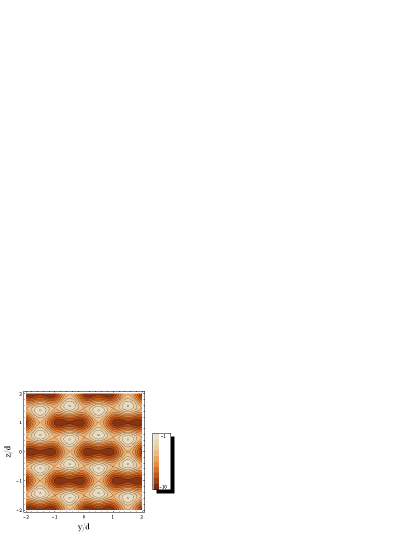
Figure 2: (Color online) Example of a double-well lattice potential in the $(y,z)$ plane. Distances are in units of the lattice spacing $d=\lambda/2$. The energy unit is $E_{R}$ (recoil energy). The $x$ direction corresponds to the ladder axes.

This kind of potential is suitable to obtain a lattice of non-frustrated ladders. Indeed, since the potential along (x,y) is separable, and Wannier functions at different sites are orthogonal, the diagonal tunneling matrix elements between wells are zero. In order to have a frustrated ladder as depicted in Fig. 1, a non-separable potential along (x,y) is required. It can be achieved by using two interfering standing waves with a blue-detuned laser along the diagonals, in the (x,y) plane. Such a potential is given for instance by:

$$V_{d}(x,y)=\big{[}\sqrt{V_{+}}\sin(\pi(x+y))+\sqrt{V_{-}}\sin(\pi(x-y))\big{]}^{2}.$$ (2)

Note that for this additional potential to be independent from the other, the laser frequency must be detuned with respect to the in-plane lasers, since all three orthogonal polarizations are already used to create the ladders. In practice all lasers are detuned in order to supress any residual interference. For simplicity, we use the same lattice spacing in the $x$ direction and thus the total optical potential is given by

$$V(x,y,z)=V_{p}(y,z)+V_{d}(x,y),$$ (3)

It describes a 3D array of frustrated 2-leg ladders. An example of the total potential is represented in Fig. 3.

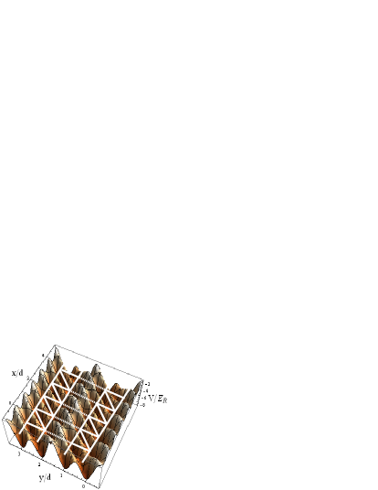
Figure 3: (Color online) Example of a potential in the $(x,y)$ plane leading to a frustrated ladder-like potential. The frustrated ladders are sketched on the potential.

III Model Hamiltonian

In the following, we assume that hopping processes and interactions leave the atoms in the lowest band. We assume that the trap is loaded with fermionic species with two different hyperfine “spin” states. In what follows, we denote these states by $\sigma=\uparrow,\downarrow$ by analogy with a spin $1/2$. From the potential written in Eq.(3), we derive an Hubbard type Hamiltonian:

$$H_{Hub} = -\sum_{i,\alpha=1,2,\sigma}t_{1}(c^{\dagger}_{i,\alpha,\sigma}c_{i+1,\alpha,\sigma}+h.c.)$$ (4)

$$- \sum_{i,\sigma}(t_{\perp}c^{\dagger}_{i,1,\sigma}c_{i,2,\sigma}+t_{2}c^{\dagger}_{i,1,\sigma}c_{i+1,2,\sigma}$$

$$~{}~{}~{}~{}+t^{\prime}_{2}c^{\dagger}_{i,2\sigma}c_{i+1,1\sigma}+h.c.)$$

$$+ \sum_{i,\alpha}(Un_{i,\alpha,\uparrow}n_{i,\alpha,\downarrow}-\mu_{i,\uparrow}n_{i,\alpha,\uparrow}-\mu_{i\downarrow}n_{i,\alpha,\downarrow}).$$

In this Hamiltonian, $c_{i,\sigma,\alpha}$ destroys an atom with “spin” index $\sigma$ on site $i$ of the chain $\alpha$, $n_{i,\alpha,\sigma}=c^{\dagger}_{i,\alpha,\sigma}c_{i,\alpha,\sigma}$ is the occupation at site $i$ of the chain $\alpha$. $t_{1},t_{\perp},t_{2},t^{\prime}_{2}$ are tunneling amplitudes as defined in Fig. 1, $U$ is a local interaction which can be controlled by Feshbach resonances and $\mu_{i\sigma}=\mu_{\sigma}-V_{i,\sigma}$ is a local chemical potential. $V_{i,\sigma}$ is the harmonic confining potential in the $x$ direction, while $\mu_{\sigma}$ is a global chemical potential for species $\sigma$. Although in real experiments the number of atoms is fixed and constant we work here in the grand-canonical ensemble, with a fixed chemical potential, in order to make a connection with magnetic systems. We assume for now that the trap is sufficiently elongated in the $x$ direction to take a constant $\mu_{i\sigma}=\mu_{\sigma}$. Then, the last term in Eq. (4) can be rewritten as

$$-\mu\sum_{i,\alpha}(n_{i,\alpha,\uparrow}+n_{i,\alpha,\downarrow})-h\sum_{i,\alpha}(n_{i,\alpha,\uparrow}-n_{i,\alpha,\downarrow}),$$

with $\mu=(\mu_{\uparrow}+\mu_{\downarrow})/2$ and

$$h=(\mu_{\uparrow}-\mu_{\downarrow})/2,$$ (5)

which are respectively equivalent to a chemical potential and an magnetic field. In what follows, when we will mention the magnetic field, we refer to an effective magnetive field given by Eq. (5). We focus on the case of strong repulsive interactions ($U\gg t_{\perp},t_{1},t_{2},t^{\prime}_{2}$) and assume half-filling, i.e. $\langle n_{i,\uparrow}+n_{i,\downarrow}\rangle=1$ in a homogeneous trap. In this limit, the system is in a Mott insulator phase with one atom per site. Charge degrees of freedom are frozen and only superexchange interactions are allowed to second order. These virtual processes lead to antiferromagnetic couplings between sites. After projecting on states with exactly one atom per site, the effective Hamiltonian for a single ladder reads:

$$H_{lad} = J_{\perp}\sum\limits_{i=1}{\bf S}_{i,1}{\bf S}_{i,2}+J_{1}\sum\limits_{i=1}\sum\limits_{\alpha=1}^{2}{\bf S}_{i,\alpha}{\bf S}_{i+1,\alpha}$$ (6)

$$+ J_{2}\sum\limits_{i=1}{\bf S}_{i,1}{\bf S}_{i+1,2}+J^{\prime}_{2}\sum\limits_{i=1}{\bf S}_{i,2}{\bf S}_{i+1,1}$$

$$- h\sum\limits_{i=1}\sum\limits_{\alpha=1}^{2}S_{i,\alpha}^{z},$$

where ${\bf S}_{i,\alpha}=\sum_{\sigma\sigma^{\prime}}c^{\dagger}_{i,\alpha,\sigma}\frac{\vec{\tau}_{\sigma\sigma^{\prime}}}{2}c_{i,\alpha,\sigma^{\prime}}$ is the “spin” operator, and $\vec{\tau}$ are the Pauli matrices. In Eq. (6), $J_{i}=4t_{i}^{2}/U>0$ denotes a superexchange coupling. We compare relative spin exchange couplings by estimating the tunneling matrix elements. We approximated the Wannier functions with the ground state of the harmonic oscillatorreview08 in the bottom of each well. With $R=0.14,V_{+}=0.1E_{R}$, $V_{-}=4E_{R}$, we found: $(t_{\perp}/t_{1})^{2}=20,\ (t_{2}/t_{1})^{2}=1.5,\ (t^{\prime}_{2}/t_{2})^{2}=10^{-5}.$ We also estimated inter-ladder couplings and found $\ (t_{2,\textrm{inter}}/t_{2})^{2}=6.10^{-3},\ (t_{1,\textrm{inter}}/t_{1})^{2}=9.10^{-3}$. >From these estimations we can infer that the ladders are very weakly coupled togethernote . Moreover, when the temperature is much larger than the interladder exchange energy, i.e. $k_{B}T\gg J_{3D}$, the ladders are effectively decoupled. In this limit, we can thus consider a single ladder-like lattice potential, as described by Hamiltonian (6).

Although we assume that the system is at half-filling i.e. that the average density per site $\rho=\rho_{\uparrow}+\rho_{\downarrow}=1$, the densities $\rho_{\uparrow}$ and $\rho_{\downarrow}$ can be quite different. In this respect, $h$ is related to the difference between the chemical potentials of both fermionic species (see Eq. (5)). The Hamiltonian thus reduces to that of an Heisenberg ladder in a magnetic field $h$. Such an Hamiltonian has been studied by various methods (e.g. see cabra97 ; chitra97 ; totsuka ; mila98 ; chaboussant98 ; chitra99 ).

Let us note that in real systems, an additional weak isotropic harmonic potential exists over the latticeschneider_04 . This confinement brings an energy offset on each lattice site and leads to an effective local chemical potential. The superfluid-insulator phase diagram is influenced by this potential. In the case where the trapping potential is spin-independent, there is no influence on the pseudo magnetic field $h$. If the interaction energy $U$ is much larger than the trapping energy $E_{\textrm{trap}}=\frac{1}{2}m\omega_{x}^{2}N_{\sigma}^{2}$, with $\omega_{x}$ the trapping frequency in the ladder direction and $N_{\sigma}$ the number of $\sigma$ atoms, one can expect a Mott insulator phase in the center of the trap, surrounded by a superfluid region.

IV Spin and charge phases

For our analysis let us start from the strong coupling limit $J_{\perp}\gg J_{1},J_{2},J^{\prime}_{2}$. This limit is clearly met within our proposed optical lattice potential.

When $J_{1}=J_{2}=J^{\prime}_{2}=0$ each rung is independent, and has four available states, a singlet and three triplets: $|S\rangle=\frac{1}{\sqrt{2}}(|\uparrow\downarrow\rangle-|\downarrow\uparrow\rangle)$, $|T_{-1}\rangle=|\downarrow\downarrow\rangle$, $|T_{0}\rangle=\frac{1}{\sqrt{2}}(|\uparrow\downarrow\rangle+|\downarrow\uparrow\rangle)$ and $|T_{1}\rangle=|\uparrow\uparrow\rangle$. Their energies are $E(S)=-3J_{\perp}/4$, $E(T_{1})=J_{\perp}/4-h$, $E(T_{0})=J_{\perp}/4$ and $E(T_{-1})=J_{\perp}/4+h$ respectively.
Upon increasing the effective magnetic field, the ground state rung magnetization $M=\langle S^{z}_{i,1}\rangle+\langle S^{z}_{i,2}\rangle$ increases up to saturation at $h=h_{c}=J_{\perp}$ where $|S\rangle$ and $|T_{1}\rangle$ become degenerate. In the presence of an inter-rung interaction the transition becomes broader and a crossover is expected between two critical fields $h_{c1}$ and $h_{c2}$.

IV.1 Special case $\rho_{\uparrow}=\rho_{\downarrow}=1/2$

IV.1.1 Repulsive interactions

In the case of half-filling with equal densities $\rho_{\uparrow}=\rho_{\downarrow}=1/2$, the strong coupling picture predicts a spin gap at zero magnetization, $M=0$. This state corresponds to a Fully Incompressible State (FIS) where both charge and spin degrees of freedom are gapped. We point out that this incompressible phase does not require non-zero couplings $J_{2},J^{\prime}_{2}$ or equivalently non-zero tunneling terms $t_{2},t^{\prime}_{2}$. Consequently, one can reach this phase with $V_{d}=0$ in the potential in Eq. (3). In the next subsection, we therefore assume $t_{2}=t^{\prime}_{2}=0$.

Let us note that the spin gap is very robust and can be theoretically obtained also in the weak coupling $J_{\perp}\ll J_{1}$ using a bosonization approach.giamarchi04

IV.1.2 Attractive interactions

The spin Hamiltonian in Eq.(4) was derived assuming strong repulsive interactions $U\gg t>0$. When $U<0$, states with zero or two atoms per site are favored. Therefore the low-energy excitations are the ones that describe the dynamics of atom pairs (in the singlet state) in a periodic potential. One may wonder whether the FIS survives at strong attractive interactions.

The correspondence is in fact quite general and can be obtained by performing the following particle-hole transformation on the initial Hubbard Hamiltonian in Eq. (4):

$$c_{i,\alpha,\uparrow} \longrightarrow c_{i,\alpha,\uparrow}$$

$$c_{i,\alpha,\downarrow} \longrightarrow (-1)^{i+\alpha}c_{i,\alpha,\downarrow}$$ (7)

This transformation affects only the “spin” $\downarrow$ atoms. Provided $t_{2}=t^{\prime}_{2}=0$, the tunneling part of the Hamiltonian is left unchanged. However, $n_{i,\alpha,\downarrow}\to(1-n_{i,\alpha,\downarrow})$. This implies therefore that $U\to-U$ in Eq. (4). The particle-hole transformation exchange the roles of $\mu$ and $h$, up to unimportant constants. Therefore, the fully gapped phase with $\rho_{\uparrow}=\rho_{\downarrow}=1/2$ that we described above from positive $U$ maps into another equivalent gapped phase at negative $U$.

Using this correspondence, one can easily infer the evolution of the average number of pairs on a rung as function of the chemical potential for $U<0$ simply by looking at the evolution of the “magnetization” with respect to the magnetic field $h$, for $U>0$. In fact half-filling corresponds to one pair of atoms per rung and to $\mu=0$. In order to increase the number of atoms beyond half-filling, one has to therefore to fill a gap of order $J_{\perp}$.

IV.2 The generic case $\rho_{\uparrow}\neq\rho_{\downarrow}$

IV.2.1 Repulsive interactions

In order to study the physics at $M\neq 0$, we follow Ref. [mila98, ] and give the main steps of the calculations leading to an effective 1D bosonic hamiltonian given in Eq. (14) for completness and readability. We first separate the Hamiltonian $H_{lad}$ into two parts, $H_{lad}=\mathcal{H}_{0}+\mathcal{H}_{1}$ with

$$\mathcal{H}_{0} = J_{\perp}\sum\limits_{i=1}^{N}{\bf S}_{i,1}{\bf S}_{i,2}-h_{c}\sum\limits_{i=1}^{N}\sum\limits_{\alpha=1}^{2}S_{i,\alpha}^{z}$$ (8)

$$\mathcal{H}_{1} = J_{1}\sum\limits_{i=1}^{N}\sum\limits_{\alpha=1}^{2}{\bf S}_{i,\alpha}{\bf S}_{i+1,\alpha}+J_{2}\sum\limits_{i=1}^{N}{\bf S}_{i,1}{\bf S}_{i+1,2}$$ (9)

$$+ J^{\prime}_{2}\sum\limits_{i=1}^{N}{\bf S}_{i,2}{\bf S}_{i+1,1}-(h-h_{c})\sum\limits_{i=1}^{N}\sum\limits_{\alpha=1}^{2}S_{i,\alpha}^{z}$$

The ground-state of $\mathcal{H}_{0}$ is $2^{N}$ degenerate. The perturbation Hamiltonian $\mathcal{H}_{1}$ will lift the degeneracy. We use standard quantum mechanics perturbation theory for degenerate ground states. Diagonalization of the perturbation Hamiltonian in the degenerate subspace yields the result to first order. One can rewrite the effective perturbative Hamiltonian for the system as:

$$\mathcal{H}_{eff}=\sum_{i=1}^{N}\left[J_{xy}\left(\sigma^{x}_{i}\sigma^{x}_{i+1}+\sigma^{y}_{i}\sigma^{y}_{i+1}\right)+J_{z}\sigma^{z}_{i}\sigma^{z}_{i+1}\right]-\tilde{h}\sum_{i=1}^{N}\sigma_{i}^{z}$$ (10)

with:

$$S_{i,1}^{+}=-\frac{1}{\sqrt{2}}\sigma_{i}^{+}~{},~{}S_{i,2}^{+}=\frac{1}{\sqrt{2}}\sigma_{i}^{+}$$

$$S_{i,1}^{-}=-\frac{1}{\sqrt{2}}\sigma_{i}^{-}~{},~{}S_{i,2}^{-}=\frac{1}{\sqrt{2}}\sigma_{i}^{-}$$

$$S_{i,1}^{z}=S_{i,2}^{z}=\frac{1}{2}(\sigma_{i}^{z}+\frac{1}{2})~{}~{},$$ (11)

and $J_{xy}=J_{1}-(J_{2}+J^{\prime}_{2})/2$, $J_{z}=J_{1}/2+(J_{2}+J^{\prime}_{2})/4$, and $\tilde{h}=h-h_{c}-J_{1}/2-(J_{2}+J^{\prime}_{2})/4$. The sigmas stand for pseudo-spin 1/2 degrees of freedom. Formally these operators are the Pauli matrices, written in the basis $\{|\uparrow\rangle_{i}=|T_{1}\rangle_{i},\ |\downarrow\rangle_{i}=|S\rangle_{i}\}$. Therefore one is able to map the original ladder system into a 1D Hamiltonian, namely the so called $XXZ$ chain. Then one can show (see for example giamarchi04 ) using a Jordan-Wigner transformation that the XXZ chain is equivalent to a single band of interacting spinless fermions. This correspondence allows us to describe low-energy properties of the XXZ chain through bosonization giamarchi04 and obtain correlation functions in this regime. Using usual bosonization formulas one finds:

$$\sigma^{z}(x)=m-\frac{1}{\pi}\partial_{x}\phi(x)+\frac{1}{2\pi\alpha}2\cos\left[2\phi(x)-\pi(2m+1)x\right],$$ (12)

$$\sigma^{+}(x)=\frac{(-1)^{x}}{\sqrt{2\pi\alpha}}e^{-i\theta(x)}\left[1+\cos\left(2\phi(x)-\pi(2m+1)x\right)\right].$$ (13)

where the bosonic fields $\phi$ and $\theta$ satisfy the commutation relation $[\phi(x),\nabla\theta(x^{\prime})]=i\pi\delta(x-x^{\prime})$. One can look at these fields as the angles of a spin $1/2$ on the Bloch sphere, with $2\phi$ being the angle taken from the $z$ axis while $\theta$ is the angle in the $XY$ plane. The commutation relation implies that order in one direction will destroy order in the other direction. Note also that $m$ is the magnetization of the $XXZ$ chain and is related to the ladder magnetization through $M=\langle S_{i,1}^{z}+S_{i,2}^{z}\rangle=m+1/2$. The form of the Hamiltonian now depends on the value of $m$. If $m\neq 0$ ($M>1/2$), it simply reads:

$$H=\frac{1}{2\pi}\int dx\left[uK\left(\partial_{x}\theta(x)\right)^{2}+\frac{u}{K}\left(\partial_{x}\phi(x)\right)^{2}\right]$$ (14)

with

$$uK = v_{F}=J_{xy}\sin(k_{F})$$ (15)

$$\frac{u}{K} = v_{F}\left(1+\frac{2J_{z}}{\pi v_{F}}(1-\cos(2k_{F}))\right)$$ (16)

$u,K$ are the so-called Luttinger parameters and control all low-energy properties of the system. Their expression in Eqs. (15-LABEL:Lutt_param3) is obtained in the limit of small $J_{z}$.

The simple quadratic form leads to a power-law decay of all correlation functions. The slowest decaying mode indicates quasi long-range order. The situation is quite different when $m=0$ ($M=1/2$). This corresponds to $\rho_{\uparrow}=3/4$ and $\rho_{\downarrow}=1/4$ in our initial fermi-fermi mixture and when the ladder-like optical lattice is loaded with this particular filling, the “spin” sector of the mixture is described by a sine-Gordon model:

$$H = \frac{1}{2\pi}\int dx\left[uK\left(\partial_{x}\theta(x)\right)^{2}+\frac{u}{K}\left(\partial_{x}\phi(x)\right)^{2}\right]$$ (18)

$$- \frac{2g_{3}}{(2\pi\alpha)^{2}}\int dx\cos\left(4\phi(x)\right),$$

where $g_{3}=J_{z}$. This signals a possible tendency towards ordering in the $z$ direction. Energetically, it is favorable to lock the angle $\phi$ so as to minimize the cosine term. However it would create large fluctuations in the $\theta$ angle therefore costing a great amount of kinetic energy. This competition can therefore lead to a phase transition at this particular filling. A renormalization group calculation will indicate whether or not the cosine term is relevant at low energy. If yes, it will favor ordering in the $z$ direction and open a spin gap. The flow equations are:

$$\frac{dK}{dl}=-y^{2}(l)K^{2}(l),\ \ \frac{dy}{dl}=(2-4K(l))y(l).$$ (19)

where we have defined $y=g_{3}/(\pi u)$. $(K=1/2,y=0)$ is a fixed point. For $K>1/2$, $dy/dl<0$ and the cosine is irrelevant. The system is therefore a Luttinger liquid, even when $M=1/2$. However, for $K<1/2$ the cosine is relevant and $y$ flows to strong coupling. A gap opens in the excitation spectrum. From the Bethe ansatz solution of the XXZ chain, one can infer that the value $K=1/2$ corresponds to the isotropic case $J_{z}=J_{xy}$ giamarchi04 . The condition $K<1/2$ is associated to the Ising phase of the XXZ Heisenberg chain i.e $J_{z}>J_{xy}$. For our original ladder system, this phase is realized when

$$J_{2}+J^{\prime}_{2}>2J_{1}/3.$$ (20)

Therefore, the opening of a “spin” gap can only occur for strong frustration.totsuka ; mila98

In what follows, we consider two cases: (i) a regular ladder with $J_{2}=J^{\prime}_{2}=0$ and (ii) a frustrated ladder with $J_{2}+J^{\prime}_{2}>2J_{1}/3$. In particular, as we have seen in Sec. II frustration can be generated in the ladder-like optical lattice with interfering standing waves along one diagonal direction (i.e. when $J_{2}=0$ or $J^{\prime}_{2}=0$).

For the weakly frustrated ladders (first case), we therefore expect “spin” correlations functions to be of Luttinger-liquid type when $\rho_{\uparrow}\neq\rho_{\downarrow}\neq 1$ while for strongly frustrated ladders (second case) we expect a “spin” gap opening for the special filling $\rho_{\uparrow}=3/4,\rho_{\downarrow}=1/4$. This situation in real space would correspond to an alternation of singlets and triplets. Such a fully incompressible state would be a direct consequence of frustration. In next section V, we will discuss how to distinguish these two phases by computing various observable.

IV.2.2 Attractive interactions

An interesting question regards the survival of the frustration-induced FIS when attractive interactions are considered. Let us then apply the particle-hole transformation defined in Eq. (IV.1.2). This transformation makes the tunneling terms along the diagonals of the ladder “spin”-dependent. More specifically, this changes the sign of the amplitudes $t_{2}$ and $t^{\prime}_{2}$ in Eq. (4) for the “spin” $\downarrow$ atoms only. There is no direct mapping between the repulsive and the attractive cases. However, one can follow a procedure similar to the one used for the repulsive case – namely a Schrieffer-Wolff transformation – starting directly from a Hamiltonian with attractive interactions, and derive a “pseudo-spin” ladder Hamiltonian quite similar to Eq. (6) but breaking the $SU(2)$ particle-hole symmetry. After projecting onto a XXZ “pseudo-spin” chain Hamiltonian similar to Eq. (10), the coupling $J_{xy}$ now becomes $J_{xy}=J_{1}+(J_{2}+J^{\prime}_{2})/2$. The condition $J_{z}>J_{xy}$ is no longer met and thus the FIS found for positive $U$ does not survive for negative $U$ in the case of a frustrated ladder.

V Observables

V.1 Density correlations.

After turning off the trap, and assuming that interactions are small, the atomic cloud evolves freely. It is possible, with laser imaging, to measure both the density $\rho(r)$ defined by

$$\rho_{t}(r)=\langle n(\mathbf{r})\rangle_{t}$$ (21)

and the density correlation function $\mathcal{G}$ defined by

$$\mathcal{G}(\mathbf{r}-\mathbf{r}^{\prime})=\langle n(\mathbf{r})n(\mathbf{r}^{\prime})\rangle_{t}-\langle n(\mathbf{r})\rangle\langle n(\mathbf{r}^{\prime})\rangle_{t},$$ (22)

after a given time of flight $t$. At zero temperature the density-density correlator is defined as follows:

$$\langle n(\mathbf{r})n(\mathbf{r}^{\prime})\rangle_{t}=\langle\Phi|U_{0}^{\dagger}(t)\Psi^{\dagger}(\mathbf{r})\Psi(\mathbf{r})\Psi^{\dagger}(\mathbf{r}^{\prime})\Psi(\mathbf{r}^{\prime})U_{0}(t)|\Phi\rangle;$$ (23)

where $|\Phi\rangle$ is the ground state inside the trap, $U_{0}^{\dagger}(t)$ is the free evolution operator and $\Psi$ is the fermionic field. As discussed in [review08, ], at sufficiently long times of flight there is a correspondence between the density in the cloud and the momentum distribution inside the trap, $\langle n(\mathbf{r})\rangle_{t}\simeq\langle n_{\mathbf{k}}\rangle_{\textrm{Trap}}$ with $\mathbf{k}=m\mathbf{r}/(\hbar t)$. In the Mott phase, with one atom per site, a measure of the density itself does not yield much information since it does not allow to distinguish species with different spins. However, one can extract interesting information about long-range order in the trap from density-density correlation functions (see Ref.[altman04, ] for a detailed calculation). In our case these correlation functions would correspond to the spin-spin correlation functions. One has indeed

$$\mathcal{G}(\mathbf{r}-\mathbf{r}^{\prime})=\mathcal{G}^{1}(\mathbf{r}-\mathbf{r}^{\prime})+\mathcal{G}^{2}(\mathbf{r}-\mathbf{r}^{\prime}),$$ (24)

with

$$\mathcal{G}^{1}(\mathbf{u}) = -\frac{1}{2}\frac{N}{W^{2}}\left(\frac{2\pi a_{0}}{a}\right)^{2}\sum_{\mathbf{G}}\delta\left(\mathbf{u}+\frac{\hbar t}{m}\mathbf{G}\right),$$ (25)

$$\mathcal{G}^{2}(\mathbf{u}) = -2\sum_{i,j}e^{i\frac{m}{\hbar t}(\mathbf{u}).(\mathbf{R}_{i}-\mathbf{R}_{j})}\langle\mathbf{S}_{i}.\mathbf{S}_{j}\rangle,$$ (26)

where $W=\hbar t/(a_{0}m)$, and $a_{0}$ is the width of the Wannier function on the lattice, $a$ is the lattice spacing and $\mathbf{G}$ is a vector of the reciprocal lattice. The first term contains the usual Bragg peaks at reciprocal lattice wave vectors, while the second term is the static spin structure factor. Density correlations in the free-falling cloud can be a probe of spin correlations inside the trap.

V.2 Result for a single ladder

In order to compute $\mathcal{G}^{2}(\mathbf{r})$, we first resort to the mapping of the ladder Hamiltonian onto the XXZ chain in the large $J_{\perp}$ limit and write:

$$\chi(k_{x},k_{y}) = \sum_{i,j}e^{i\mathbf{k}.(\mathbf{R}_{i}-\mathbf{R}_{j})}\langle\mathbf{S}_{i}.\mathbf{S}_{j}\rangle$$

$$= \frac{1}{2}(1+\cos k_{y}a)\sum_{i,j}e^{ik_{x}(X_{i}-X_{j})}\langle\mathcal{M}^{z}_{i}\mathcal{M}^{z}_{j}\rangle$$

$$+ (1-\cos k_{y}a)\sum_{i,j}e^{ik_{x}(X_{i}-X_{j})}\langle\sigma^{+}_{i}\sigma^{-}_{j}\rangle,$$

$$= \frac{1}{2}(1+\cos k_{y}a)\chi_{zz}(k_{x})+(1-\cos k_{y}a)\chi_{+-}(k_{x}).$$

where $i,j$ are the rung indices, $X_{i}$ is the position of rung $i$ along the longitudinal direction, $\mathcal{M}_{i}^{z}=S^{z}_{i,1}+S^{z}_{i,2}$ and the variables $\sigma_{i}$ have been defined in Eq. (IV.2.1). It is worth emphasizing that a $y$-dependent geometrical factor appears before each sum, which means that for special values of $k_{y}$, i.e. special positions of observation inside the cloud, one can preferentially observe rung-rung or transverse correlations. The correlators $\langle\mathcal{M}^{z}_{i}\mathcal{M}^{z}_{j}\rangle$ and $\langle\sigma^{+}_{i}\sigma^{-}_{j}\rangle$ can be computed at zero temperature in the Luttinger liquid phase using bosonization. While the correlators are easy to compute in the Luttinger liquid phase, the calculation is much more involved in the FIS. Generally one has:

$$\langle\mathcal{M}^{z}(x)\mathcal{M}^{z}(0)\rangle=M^{2}+\frac{1}{\pi^{2}}\langle\partial_{x}\phi(x)\partial_{x}\phi(0)\rangle+\frac{2}{(2\pi\alpha)^{2}}\cos(2\pi Mx)\langle\cos(2\phi(x))\cos(2\phi(x))\rangle,$$ (28)

$$\langle\sigma^{+}(x)\sigma^{-}(0)\rangle=\frac{1}{\pi\alpha}\langle e^{i\theta(x)}e^{-i\theta(0)}\cos\left[2\phi(x)-\pi(2M-1)x\right]\cos\left[2\phi(0)\right]\rangle+\frac{\cos\pi x}{2\pi\alpha}\langle e^{i\theta(x)}e^{-i\theta(0)}\rangle.$$ (29)

Before computing explicitly those correlation functions, one remark can be made about the general form of $\chi(k_{x},k_{y})$. We have to compute sums of the form $\sum_{i,j}e^{i\kappa(i-j)a}f(|i-j|)$, where $a$ is the lattice spacing and $i,j$ are integers running from $1$ to $N$, the length of a ladder. It is easily shown that:

$$\sum_{i,j=1}^{N}e^{i\kappa(i-j)a}f(|i-j|)=Nf(0)+2\sum_{p=1}^{N-1}(N-p)\cos(p\kappa a)f(p).$$ (30)

The maximum value $Nf(0)+2\sum_{p}(N-p)f(p)$ of the sum is obtained for $\kappa\equiv 0[\frac{2\pi}{a}]$. Its minimum value is $Nf(0)+2\sum_{p}(N-p)(-1)^{p}f(p)$ and it is reached when $\kappa\equiv\frac{\pi}{a}[\frac{2\pi}{a}]$. The height of the peaks is partly controlled by the longitudinal size of the ladders.

V.3 Correlation functions in the Luttinger liquid phase

As indicated earlier, in the Luttinger liquid phase, i.e. for $M\neq 1/2$ or $M=1/2$ but weak frustration, all correlation functions decay as power laws, in accordance with the quasi-1D character of the ladders. The rung-rung correlation function reads:

$$\langle\mathcal{M}^{z}(x)\mathcal{M}^{z}(0)\rangle=M^{2}+\frac{K}{2\pi^{2}}\frac{1}{x^{2}}+\frac{2}{(2\pi\alpha)^{2}}\cos(2\pi Mx)\left(\frac{\alpha}{x}\right)^{2K},$$ (31)

As for the staggered correlation functions (intrachain and interchain), they are embedded in:

$$\langle\sigma^{+}(x)\sigma^{-}(0)\rangle=\frac{1}{\pi\alpha}\cos\left(\pi(2M-1)x\right)\left(\frac{\alpha}{x}\right)^{2K+1/2K}+\frac{\cos\pi x}{2\pi\alpha}\left(\frac{\alpha}{x}\right)^{1/2K}.$$ (32)

The rung-rung correlation in equation (31) contains two type of terms: a Fermi liquid like mode around $q=0$, and another contribution at an incommensurate mode with wave vector $q=2\pi M$. This mode decays as a power-law with a non-universal exponent which depends on the interactions. The $XY$ correlations display power-law decays for two modes, $q=\pi$ and $q=2M-1$. Since $K>1/2$, the slowest decaying mode is the antiferromagnetic one (i.e. $q=\pi$) in the $XY$ correlator. These properties are reflected through several peaks in $\chi_{zz}$ (Fig. 4) and $\chi_{+-}$ (Fig. 5). Due to the power-law decay of correlations these are broad peaks, as opposed to usual Bragg peaks appearing in $\mathcal{G}_{1}$. Most of them appear at incommensurate vectors, shifted from reciprocal lattice vectors by values depending on the magnetization $M$. The sharper and higher peaks appear in the staggered correlation function at half the reciprocal lattice vectors, indicating quasi-long range antiferromagnetic order in the $XY$ plane.

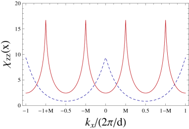
Figure 4: (Color online) Rung contribution in the spin part of the density correlations (see Eq. (31)), in the Luttinger liquid phase. $k_{x}$ is in unit of $2\pi/d$. $\chi_{zz}$ in dimensionless. We observe two sets of broad peaks: One at reciprocal lattice vectors, the other shifted by $\pm M$ (see text). Here we have taken $M=1/4$, $K=0.6$ and a ladder with 100 rungs.

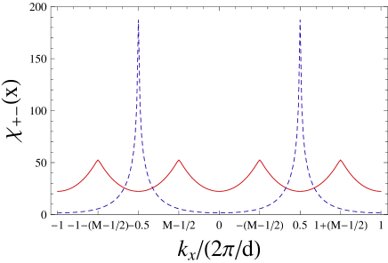
Figure 5: (Color online) Staggered contribution in the spin part of the density correlations (see Eq. (32)), in the Luttinger liquid phase. $k_{x}$ is in unit of $2\pi/d$. $\chi_{+-}$ in dimensionless. We also observe two sets of broad peaks. One is shifted by $\pm(M-1/2)$ with respect to reciprocal lattice vectors, the other is at half the reciprocal lattice vectors (see text). The latter is the most prominent, indicating quasi long-range antiferromagnetic order in the XY plane.

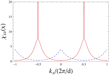
Figure 6: (Color online) Rung contribution in the spin part of the density correlations, in the FIS. $k_{x}$ is in unit of $2\pi/d$. Former incommensurate peaks coalesce into Bragg peaks at half-reciprocal lattice vectors. Former peaks at reciprocal lattice vectors are rounded. Here $M=1/2$, $K=0.25$

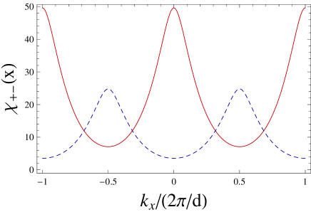
Figure 7: (Color online) Staggered contribution in the spin part of the density correlations, in the FIS. $k_{x}$ is in unit of $2\pi/d$. Incommensurate peaks coalesce to reciprocal lattice vectors. All peaks get rounded by the exponential damping of the modes.

V.4 Correlation functions in the fully incompressible state

In the FIS, the system opens a spin gap, and excitations are now described by a sine-Gordon (sG) Hamiltonian:

$$H_{boson} = \frac{1}{2\pi}\int dx\left[uK\left(\partial_{x}\theta(x)\right)^{2}+\frac{u}{K}\left(\partial_{x}\phi(x)\right)^{2}\right]$$ (33)

$$- \frac{2g_{3}}{(2\pi\alpha)^{2}}\int dx\cos\left(4\phi(x)\right).$$

Every excitation of the sG model is massive and will therefore lead to exponentially decaying correlations. To gain some insight on the precise form of correlators, let us remember that the sine-Gordon Hamiltonian is obtained from the $XXZ$ chain Hamiltonian

$$H_{XXZ}=\sum_{i=1}^{N}\left[J_{xy}\left(\sigma^{x}_{i}\sigma^{x}_{i+1}+\sigma^{y}_{i}\sigma^{y}_{i+1}\right)+J_{z}\sigma^{z}_{i}\sigma^{z}_{i+1}\right].$$ (34)

Since the $J_{xy}$ interaction is frozen on the plateau, the physics is that of the Ising model in $1+1$ dimension, away from criticality. One can map the latter model to free Majorana fermions, and correlations can be computed exactly. A theory of free Majorana fermions is obtained from the sine-Gordon model, for $K=1/4$. One intuitive way to look at the problem is to use the Luther-Emery trickluther and make a change of variable $\tilde{\phi}\rightarrow\phi/\sqrt{K}$, that transforms the cosine operator into $\cos 2\tilde{\phi}$, which is a simple backscattering term in the fermion language. The resulting refermionized Hamiltonian is that of two species of fermions, right-moving and left-moving, with back-scattering – that in turn can be written in terms of free Majorana fermions. Using this trick one is able to compute $\langle e^{i\theta(x)}e^{-i\theta(0)}\rangle$ exactly:

$$\langle e^{i\theta(x,\tau)}e^{-i\theta(0,0)}\rangle = \left(\frac{\Delta}{u}\right)^{2}\left[K_{1}\left(\frac{\Delta}{u}\sqrt{x^{2}+\alpha^{2}}\right)^{2}\right.$$ (35)

$$- \left.K_{0}\left(\frac{\Delta}{u}\sqrt{x^{2}+\alpha^{2}}\right)^{2}\right],$$

where $K_{0}$ and $K_{1}$ are modified Bessel functions of the second kind. The short distance behavior of this function is simply $(x^{2}+\alpha^{2})^{-1}$. This coincides with the Luttinger liquid result, as $K=1/4$ on the plateau. However at large distances, it decays exponentially. In $\chi_{+-}$, former sharp peaks at half reciprocal lattice vectors are greatly reduced and loose their cusp while incommensurate peaks coalesce at reciprocal lattice vectors, losing their cusp as well (see Fig. 7). In order to get $\langle\cos(2\phi(x))\cos(2\phi(0))\rangle$, we use the same refermionization procedure and mapping to the 2D Ising model off criticality (see [tsvelik, ], chap. 18, for details) and obtain

$$\langle\cos 2\phi(x)\cos 2\phi(0)\rangle\simeq\left(1+2K^{2}K_{0}\left(\frac{\Delta}{u}\sqrt{x^{2}+\alpha^{2}}\right)^{2}\right).$$ (36)

We thus find that the function $\langle\cos(2\phi(x))\cos(2\phi(0))\rangle$ decays exponentially to 1. As a consequence the former incommensurate broad peaks in $\chi_{zz}$ coalesce into sharp Bragg peaks at half reciprocal lattice wave vectors (see Fig. 6). Using the following formula

$$\langle\mathcal{T}_{\tau}\partial_{x}\phi(x,\tau)\partial_{x}\phi(0,0)\rangle=\lim_{\eta\rightarrow 0}\frac{1}{\eta^{2}}\partial_{x}^{2}\langle e^{i\eta\phi(x,\tau)}e^{-i\eta\phi(0,0)}\rangle,$$ (37)

one explicitly finds at zero temperature:

$$\langle\partial_{x}\phi(x)\partial_{x}\phi(0)\rangle = \frac{K\Delta^{2}}{4u^{2}}\left[K_{0}\left(\frac{\Delta}{u}\sqrt{x^{2}+\alpha^{2}}\right)\right.$$ (38)

$$+ \left.K_{2}\left(\frac{\Delta}{u}\sqrt{x^{2}+\alpha^{2}}\right)\right].$$

At short distances $\langle\partial_{x}\phi(x)\partial_{x}\phi(0)\rangle$ behaves as $(x^{2}+\alpha^{2})^{-1}$ just as in the Luttinger liquid phase, but it is exponentially suppressed at large distances. In $\chi_{zz}$ former peaks at reciprocal lattice vectors change shape by loosing their cusp (Fig. 6). To summarize, the appearance of Bragg peaks at half reciprocal lattice vectors in $\chi_{zz}$ and the clear damping of these modes in $\chi_{+-}$ indicates antiferromagnetic ordering in the $z$ direction which corresponds in that case to an alternation of singlets and triplets on the rungs of a ladder.

VI Conclusions

In summary, frustrated spin ladders can be simulated by an optical superlattice. We have shown that a phase transition from the spin liquid to a fully incompressible phase or magnetically ordered phase is possibly realized through adjusting the lattice parameters controlled by laser beams. The spin-gapped state is expected to occur at sufficiently low temperatures $T$, less than the gap $\Delta$. From the study of section IV it appears that $\Delta$ is of the order of $J_{1}$. Therefore, the observation of this state demands the same kind of experimental challenge on temperature as the realization of the N el phase in an optical lattice. Provided temperature is low enough, the coalescence of incommensurate peaks in the staggered and longitudinal density-density correlation functions into Bragg peaks at half-reciprocal or reciprocal lattice vectors would provide a concrete signature for the observation of the transition. Our results show that strongly correlated cold atoms in optical lattices provide a route to observe this quantum phase transition. Manipulating the amplitudes and wave vectors of laser beams, the coupling between spins can be adjusted in a wide range. Recent developments of controlling the cold atoms in optical lattices allow for the experimental investigation of our prediction in the future.

Acknowledgements: We would like to acknowledge fruitful discussions with N. Laflorencie.

References

- (1) E. Jané, G. Vidal, W. Dürr, P. Zoller, and J. I. Cirac, Quant. Inf. Comp. 3, 15 (2003).
- (2) A. B. Kuklov and B. V. Svistunov, Phys. Rev. Lett. 90, 100401 (2003).
- (3) L.-M. Duan, E. Demler, and M. D. Lukin, Phys. Rev. Lett. 91, 090402 (2003).
- (4) J. J. Garcia-Ripoll and J. I. Cirac, New Journal of Physics 5 76 (2003).
- (5) S. K. Yip, Phys. Rev. Lett., 90 250402 (2003).
- (6) J. J. Garcia-Ripoll, M. A. Martin-Delgado, and J. I. Cirac, Phys. Rev. Lett. 93 250405 (2004).
- (7) L. Santos, M. A. Baranov, J. I. Cirac, H.-U. Everts, H. Fehrmann, and M. Lewenstein, Phys. Rev. Lett. 93, 030601 (2004)
- (8) M. Polini, R. Fazio, A. H. MacDonald, and M. P. Tosi, Phys. Rev. Lett. 95(1), 010401 (2005).
- (9) S. Gopalan, T. M. Rice, and M. Sigrist, Phys. Rev. B 49 8901 (1994).
- (10) M. Azuma, Z. Hiroi, M. Takano, K. Ishida, and Y. Kitaoka, Phys. Rev. Lett., 73 3463 (1994).
- (11) J.S. Miller and A. J. Epstein, Angewandte Chemie International Edition in English, 33, 385 (1994).
- (12) P. B. Blakie et al., J. Phys. B 37, 1391 (2004).
- (13) K. I. Petsas, A. B. Coates, and G. Grynberg, Phys. Rev. A 50, 5173 (1994).
- (14) W. P. Zhang, HanPu, C. Search, and P. Meystre, Phys. Rev. Lett. 88, 060401 (2002); Z. W. Xie, W. Zhang, S. T. Chui, and W. M. Liu, Phys. Rev. A 69, 053609 (2004).
- (15) P. Buonsante, V. Penna, and A. Vezzani, Phys. Rev. A 70, 061603(R) (2004); 72, 031602 (2005).
- (16) S. Trebst, U. Schollwock, M. Troyer, and P. Zoller, Phys. Rev. Lett. 96, 250402 (2006).
- (17) A. Micheli, G. K. Brennen, and P. Zoller, Nature Physics 2, 341 (2006).
- (18) G. Modugno, F. Ferlaino, R. Heidemann, G. Roati, and M. Inguscio, Phys. Rev. A 68, 011601(R) (2003); G. Roati, E. de Mirandes, F. Ferlaino, H. Ott, G. Modugno, and M. Inguscio, Phys. Rev. Lett. 92, 230402 (2004); L. Pezze, L. Pitaevskii, A. Smerzi, S. Stringari, G. Modugno, E. De Mirandes, F. Ferlaino, H. Ott, G. Roati, and M. Inguscio, ibid. 93, 120401 (2004).
- (19) M. Kohl, H. Moritz, T. Stoferle, K. Gunter, and T. Esslinger, Phys. Rev. Lett. 94, 080403 (2005); T. Stoferle, H. Moritz, K. Gunter, M. Kohl, and T. Esslinger, ibid. 96, 030401 (2006).
- (20) J. K. Chin et al., Nature (London) 443, 961 (2006).
- (21) A. E. Feiguin and F. Heidrich-Meisner, Phys. Rev. Lett. 102, 076403 (2009).
- (22) Y. Fujihara, A. Koga, and N. Kawakami, Phys. Rev. A 79, 013610 (2009)
- (23) J. Sebby-Strabley, M. Anderlini, P.S. Jessen and J.V. Porto, Phys. Rev. A 73, 033605 (2006).
- (24) P. J. Lee, M. Anderlini, B. L. Brown, J. Sebby-Strabley, W. D. Phillips, and J.V. Porto, Phys.Rev.Lett. 99, 020402 (2007).
- (25) I. Bloch, J. Dalibard, and W. Zwerger, Rev. Mod. Phys. (2008)
- (26) Let us also note that while rigorously the potential (3) would have , we keep it for generalities in our model Hamiltonian.
- (27) D. C. Cabra, A. Honecker, and P. Pujol, Phys. Rev. Lett. 79, 5126 (1997); Phys. Rev. B 58, 6241 (1998).
- (28) R. Chitra and T. Giamarchi, Phys. Rev. B 55, 5816 (1997).
- (29) K. Totsuka, Phys. Rev. B 57, 3454 (1998).
- (30) F. Mila, Eur. Phys. J. B, 6, 201 (1998).
- (31) G. Chaboussant et al. Eur. Phys. J. B 6, 167 (1998).
- (32) T. Giamarchi and A.M. Tsvelik , Phys. Rev. B 59, 11398 (1999).
- (33) U. Schneider et al., Science 322, 1520 (2008).
- (34) T. Giamarchi, Quantum Physics in One Dimension, Oxford University Press, Oxford (2004).
- (35) E. Altman, E. Demler and M. D. Lukin, Phys. Rev. A 70, 013603 (2004).
- (36) A. Luther and V. J. Emery, Phys. Rev. Lett. 33, 589 (1974).
- (37) A. O. Gogolin, A. A. Nersesyan, and A. M. Tsvelik, Bosonization and Strongly Correlated Systems, Cambridge University Press (1998).