Statistics of linear families of smooth functions on knots

Abstract.

Given a knot $K$ in an Euclidean space ${\mathbb{R}}^{n}$, and a finite dimensional subspace ${\boldsymbol{V}}\subset C^{\infty}(K)$, we express the expected number of critical points of a random function in ${\boldsymbol{V}}$in terms of an integral-geometric invariant of $K$ and ${\boldsymbol{V}}$. When ${\boldsymbol{V}}$ consists of the restrictions to $K$ of homogeneous polynomials of degree $\ell$ on ${\mathbb{R}}^{n}$, this invariant takes the form of total curvature of a certain immersion of $K$. In particular, when $K$ is the unit circle in ${\mathbb{R}}^{2}$ centered at the origin, then the expected number of critical points of the restriction to $K$ of a random homogeneous polynomial of degree $\ell$ is $2\sqrt{3\ell-2}$, and the expected number of critical points on $K$ of a random trigonometric polynomial of degree $k$ is approximately $1.549k$.

To the memory of my mathematical hero, Vladimir Igorevich Arnold

Introduction

A celebrated result of Fáry and Milnor [2, 5] states that the expected number of critical points of the restriction to a knot $K\hookrightarrow{\mathbb{R}}^{3}$ of a random linear map $h:{\mathbb{R}}^{3}\rightarrow{\mathbb{R}}$ is equal to an integral-geometric invariant of the knot, namely, its (suitably normalized) total curvature. It is natural to ask how this result changes if, instead of random linear maps, we look at random homogeneous polynomials $P:{\mathbb{R}}^{3}\rightarrow{\mathbb{R}}$ of a given degree $\ell$. It is convenient to investigate an even more general situation.

Suppose that ${\boldsymbol{U}}$ is an oriented real Euclidean space of dimension $n$ and $K\hookrightarrow{\boldsymbol{U}}$ is a knot in ${\boldsymbol{U}}$, i.e., an smoothly embedded $S^{1}$. We assume that $0\not\in K$. For any positive integer $\ell$ we denote by $\mathcal{Q}_{\ell}({\boldsymbol{U}})$ the space of symmetric $\ell$-linear forms on ${\boldsymbol{U}}$. Each such form defines a polynomial function

$$P_{\Phi}:{\boldsymbol{U}}\rightarrow{\mathbb{R}},\;\;P_{\Phi}({\boldsymbol{u}})=\Phi(\underbrace{{\boldsymbol{u}},\dotsc,{\boldsymbol{u}}}_{\ell}).$$

We denote by $f_{\Phi}$ the restriction of $P_{\Phi}$ to the knot $K$. We will refer to such functions as polynomial functions on $K$ of degree $\ell$. For random $\Phi$, the function $f_{\Phi}$ is Morse, and we denote by $\mu_{K}^{\ell}(\Phi)$ its number of critical points. We can regard $\mu_{K}(\Phi)$ as a random variable and ask how is its expectation related to the global geometry of $K$.

To describe this relationship, denote by $\mathcal{S}^{\ell}$ the unit sphere in $\mathcal{Q}_{\ell}({\boldsymbol{U}})$ with respect to the natural metric $\langle-,-\rangle_{\ell}$ induced by the Euclidean metric on ${\boldsymbol{U}}$. The expected number of critical points of $f_{\Phi}$ is the real number $\mu_{K}^{\ell}$ defined by

$$\mu_{K}^{\ell}=\frac{1}{{\rm area}\,(\mathcal{S}^{\ell})}\int_{\mathcal{S}^{\ell}}\mu_{K}^{\ell}(\Phi)\,dS(\Phi).$$

In Theorem 2.1 we express $\mu_{K}^{\ell}$ as an integral geometric invariant of $K$. This invariant is described in terms of the Veronese map $\mathcal{V}_{\ell}:{\boldsymbol{U}}\rightarrow\mathcal{Q}_{\ell}({\boldsymbol{U}})$ uniquely determined by the equality

$$\bigl{\langle}\,\Phi,\mathcal{V}_{\ell}({\boldsymbol{u}})\,\bigr{\rangle}_{\ell}=\Phi(\underbrace{{\boldsymbol{u}},\dotsc,{\boldsymbol{u}}}_{\ell}),\;\;\forall{\boldsymbol{u}}\in{\boldsymbol{U}},\;\;\Phi\in\mathcal{Q}_{\ell}({\boldsymbol{U}}).$$

The restriction of the Veronese map to $K$ produces an immersion

$$\mathcal{V}_{\ell}:K\rightarrow\mathcal{Q}_{\ell}({\boldsymbol{U}})$$

that we called the $\ell$-th Veronese immersion of $K$. In Theorem 2.1 we show that $\mu_{K}^{\ell}$ is the total curvature of the $\ell$-th Veronese immersion. The case $\ell=1$ of this theorem is the celebrated result of Fáry and Milnor [2, 5].

As an application we compute $\mu_{K}^{\ell}$, when $K$ is the unit circle in ${\mathbb{R}}^{2}$ centered at the origin. More precisely, we show that in this case $\mu^{\ell}_{K}=2\sqrt{3\ell-2}$. In other words, the expected number of critical points of a polynomial function on $K$ of degree $\ell$ is $2\sqrt{3\ell-2}$.

We obtain Theorem 2.1 as a special case of Theorem 1.1 that describes the expected number of critical points of a random function belonging to a fixed finite dimensional subspace ${\boldsymbol{V}}\subset C^{\infty}(K)$ satisfying a nondegeneracy condition (1.1).

Theorem 1.1 has another interesting consequence. More precisely, in Theorem $\hbox to0.0pt{$\sqcap$\hss}\sqcup$ ‣ 4.1 we show that the expected number of critical points on the unit circle of a random trigonometric polynomial of degree $n$ is

$$T_{n}=2\sqrt{\frac{3\beta_{5}(n+1)}{5\beta_{3}(n+1)}},$$

where $\beta_{k}$ denotes the $k$-th Bernoulli polynomial. In particular

$$T_{n}\sim 2n\sqrt{\frac{3}{5}}\;\;\mbox{as $n\rightarrow\infty$}.$$

✍ Notations. We will denote by $\boldsymbol{\sigma}_{n}$ the “area” of the round $n$-dimensional sphere $S^{n}$ of radius $1$, and by $\boldsymbol{\omega}_{n}$ the “volume” of the unit ball in ${\mathbb{R}}^{n}$. These quantities are uniquely determined by the equalities (see [7, Ex. 9.1.11])

$$\boldsymbol{\sigma}_{n-1}=n\boldsymbol{\omega}_{n},\;\;\boldsymbol{\omega}_{n}=\frac{\Gamma(1/2)^{n}}{\Gamma(1+n/2)},\;\;\Gamma(1/2)=\sqrt{\pi},$$

where $\Gamma$ is Euler’s Gamma function.

1. An abstract result

Let ${\boldsymbol{U}}$ and ${\boldsymbol{V}}$ be a real, oriented Euclidean space of dimension $n$. We denote by $(-,-)_{\boldsymbol{U}}$ the inner product in ${\boldsymbol{U}}$ and by $S({\boldsymbol{U}})$ the unit sphere in ${\boldsymbol{U}}$. Suppose that $K\hookrightarrow{\boldsymbol{U}}$ is a smooth knot in ${\boldsymbol{U}}$, i.e., the image of a smooth embedding $S^{1}\hookrightarrow{\boldsymbol{U}}$. Fix an arclength parametrization of $K$

$$s\mapsto{\boldsymbol{x}}(s),\;\;0\leq s\leq L,$$

where $L$ denotes the length of $K$.

Assume that we are given a finite dimensional subspace ${\boldsymbol{V}}\subset C^{\infty}({\boldsymbol{U}})$ of dimension $N$ satisfying the nondegeneracy condition

$$\forall s\in[0,L],\;\;\exists\boldsymbol{v}\in{\boldsymbol{V}}:\;\;d_{{\boldsymbol{x}}(s)}\boldsymbol{v}({\boldsymbol{x}}^{\prime}(s))\neq 0,$$ (1.1)

where $d_{\boldsymbol{x}}\boldsymbol{v}$ denotes the differential of the function $\boldsymbol{v}$ at ${\boldsymbol{x}}$. We fix an Euclidean inner product $(-,-)_{\boldsymbol{V}}$ on ${\boldsymbol{V}}$ and we denote by $S({\boldsymbol{V}})$ the unit sphere in ${\boldsymbol{V}}$ centered at the origin.

As explained in [7, §1.2], the condition (1.1) implies that for generic $\boldsymbol{v}\in{\boldsymbol{V}}$, the restriction of the function $\boldsymbol{v}$ to $K$ is a Morse function. We denote by $\mu_{K}(\boldsymbol{v})$ its number of critical points. Note that for any nonzero scalar $t\in{\mathbb{R}}$ the restriction of $t\boldsymbol{v}$ to $K$ is Morse if and only if the restriction of $\boldsymbol{v}$ to $K$ is such. Thus, it suffices to concentrate on functions $\boldsymbol{v}\in S({\boldsymbol{V}})$. The main goal of this section is the computation of the expected number of critical points of a random function in $S({\boldsymbol{V}})$, i.e., the quantity

$$\mu_{K}^{\boldsymbol{V}}:=\frac{1}{{\rm area}\,\bigl{(}\,S({\boldsymbol{V}})\,\bigr{)}}\int_{S({\boldsymbol{V}})}\mu_{K}(\boldsymbol{v})\,|dS(\boldsymbol{v})|=\frac{1}{|}{\boldsymbol{\sigma}_{N-1}\bigl{(}\,S({\boldsymbol{V}})\,\bigr{)}}\int_{S({\boldsymbol{V}})}\mu_{K}(\boldsymbol{v})\,|dS(\boldsymbol{v})|,$$

where $|dS|$ is the “area” density on $S({\boldsymbol{V}})$.

To describe the result we need to introduce the main characters. Set ${\boldsymbol{V}}{{}^{\vee}{}}:=\operatorname{Hom}({\boldsymbol{V}},{\mathbb{R}})$ and observe that we have a smooth map $\xi:K\rightarrow{\boldsymbol{V}}{{}^{\vee}{}}$ that associates to each point ${\boldsymbol{x}}(s)\in K$ the linear map

$$\xi_{s}:{\boldsymbol{V}}\rightarrow{\mathbb{R}},\;\ \;\boldsymbol{v}\mapsto d_{{\boldsymbol{x}}(s)}\boldsymbol{v}({\boldsymbol{x}}^{\prime}(s))\in{\mathbb{R}}.$$ (1.2)

Using the metric induced isomorphism ${\boldsymbol{V}}{{}^{\vee}{}}\rightarrow{\boldsymbol{V}}$ we obtain a dual map

$$\xi^{\dagger}:K\rightarrow{\boldsymbol{V}}.$$ (1.3)

The nondegeneracy condition (1.1) implies that $\xi^{\dagger}_{s}\neq 0$, $\forall s$. We can thus define a smooth map

$${\boldsymbol{\nu}}:K\rightarrow S({\boldsymbol{V}}),\;\;{\boldsymbol{\nu}}(s):=\frac{1}{|\xi^{\dagger}_{s}|}\xi_{s}.$$

Theorem 1.1.

Let ${\boldsymbol{U}}$, $K$ and ${\boldsymbol{V}}$ be as above then

$$\mu_{K}^{\boldsymbol{V}}:=\frac{1}{\boldsymbol{\sigma}_{N-1}}\int_{S({\boldsymbol{V}})}\mu_{K}(\boldsymbol{v})\,|dS(\boldsymbol{v})|=\frac{1}{\pi}\int_{K}|\nu^{\prime}(s)|\,|ds|.$$

Proof.

Set

$$E_{\boldsymbol{\nu}}:=\bigl{\{}\,({\boldsymbol{x}},\boldsymbol{v})\in K\times S({\boldsymbol{V}});\;\;{\boldsymbol{\nu}}({\boldsymbol{x}})\perp\boldsymbol{v}\,\bigr{\}}.$$

Note that $E_{\boldsymbol{\nu}}$ can be alternatively defined as the zero set of the function

$$F:K\times S({\boldsymbol{V}})\rightarrow{\mathbb{R}},\;\;F({\boldsymbol{x}},\boldsymbol{v})=({\boldsymbol{\nu}}(x),\boldsymbol{v})_{\boldsymbol{V}},$$

and the differential of $F$ is nonzero along the level set $\{F=0\}$. This shows that $E_{\boldsymbol{\nu}}$ is a smooth submanifold of $K\times S({\boldsymbol{V}})$ and

$$\dim E_{\boldsymbol{\nu}}=\dim S({\boldsymbol{V}})=N-1.$$

We denote by $g_{E}$ the metric on $E_{\boldsymbol{\nu}}$ induced by the natural metric of $K\times S({\boldsymbol{V}})$, and by $|dV_{E}|$ the associated volume density. We have two natural (left and right) smooth maps

$$K\stackrel{{\scriptstyle\lambda}}{{\longleftarrow}}E_{{\boldsymbol{\nu}}}\stackrel{{\scriptstyle\rho}}{{{\longrightarrow}}}\boldsymbol{S}(V).$$

The fiber of $\lambda$ over ${\boldsymbol{x}}\in K$ is the Equator

$$E_{\boldsymbol{x}}:=\bigl{\{}\boldsymbol{v}\in S({\boldsymbol{V}});\;\;\boldsymbol{v}\perp{\boldsymbol{\nu}}(x)\,\bigr{\}},$$

while the fibers of $\rho$ are generically finite. Tautologically, the restriction of $\lambda$ to any fiber of $\rho$ is injective. More importantly, for any $\boldsymbol{v}\in S({\boldsymbol{V}})$ the subset $\lambda\bigl{(}\rho^{-1}(\boldsymbol{v}))\subset K$ is the set of critical points of the restriction of $\boldsymbol{v}$ to $K$. Hence, for generic $\boldsymbol{v}\in{\boldsymbol{V}}$ we have

$$\mu_{K}(\boldsymbol{v})=\#\rho^{-1}(\boldsymbol{v}).$$

We have thus reduced the problem to computing the average number of points in the fibers of $\rho$ in terms of integral-geometric invariants of the map ${\boldsymbol{\nu}}$. We will achieve this in (1.10).

The area formula (see [3, §3.2] or [4, §5.1]) implies that

$$\int_{S({\boldsymbol{V}})}\#\rho^{-1}(\boldsymbol{w})|dS(\boldsymbol{v})|=\int_{E}J_{\rho}(x,\boldsymbol{v})|dV_{E}(x,\boldsymbol{v})|,$$ (1.4)

where the nonnegative function $J_{\rho}$ is the Jacobian of $\rho$ defind by the equality

$$\rho^{*}|dS|=J_{\rho}\cdot|dV_{E}|.$$

To compute the integral in the right-hand side of (1.4) we need a more explicit description of the geometry of $E_{\boldsymbol{\nu}}$.

Let $({\boldsymbol{x}}_{0},\boldsymbol{v}_{0})\in E_{\boldsymbol{\nu}}$. Fix an orthonormal frame $e_{1},\dotsc,e_{N-2}$ of the tangent space of $E_{{\boldsymbol{x}}_{0}}$ at $\boldsymbol{v}_{0}$. Assume ${\boldsymbol{x}}_{0}={\boldsymbol{x}}(s_{0})$. Then the tangent space of $E_{\boldsymbol{\nu}}$ at $({\boldsymbol{x}}_{0},\boldsymbol{v}_{0})$ consists of tangent vectors

$$\dot{s}{\boldsymbol{x}}^{\prime}(s_{0})\oplus\dot{\boldsymbol{v}}\in T_{{\boldsymbol{x}}_{0}}K\oplus T_{\boldsymbol{v}_{0}}S({\boldsymbol{V}}),\;\;\dot{s}\in{\mathbb{R}},$$

such that

$$\dot{s}({\boldsymbol{\nu}}^{\prime}(s_{0}),\boldsymbol{v}_{0})_{\boldsymbol{V}}+(\nu(s_{0}),\dot{\boldsymbol{v}})_{{\mathbb{V}}}=0.$$ (1.5)

Define

$$e_{0}={\boldsymbol{x}}^{\prime}(s)-({\boldsymbol{\nu}}^{\prime}(s_{0}),\boldsymbol{v}_{0})_{\boldsymbol{V}}{\boldsymbol{\nu}}(s_{0}).$$

For simplicity we set

$$\mu({\boldsymbol{x}}_{0},\boldsymbol{v}_{0}):=\bigl{|}\,({\boldsymbol{\nu}}^{\prime}(s_{0}),\boldsymbol{v}_{0})_{\boldsymbol{V}}\,\bigr{|}.$$

The equality (1.5) implies that the collection

$$e_{0},e_{1},\dotsc,e_{N-2}$$

is an orthogonal basis of $T_{({\boldsymbol{x}}_{0},\boldsymbol{v}_{0})}E_{{\boldsymbol{\nu}}}$. Moreover, the length of $e_{0}$ is

$$|e_{0}|=\sqrt{1+\mu({\boldsymbol{x}}_{0},\boldsymbol{v}_{0})^{2}}.$$

If we denote by $dS_{\boldsymbol{x}}$ the area form on $E_{\boldsymbol{x}}$ then we see that at $({\boldsymbol{x}}_{0},\boldsymbol{v}_{0})$ we have

$$ds\wedge dS_{\boldsymbol{x}}(e_{0},e_{1},\dotsc,e_{N-2})=\pm 1.$$

Hence at $({\boldsymbol{x}}_{0},\boldsymbol{v}_{0})$ we have

$$|dV_{E}|=|e_{0}|\cdot|ds\wedge dS_{\boldsymbol{x}}|=\sqrt{1+\mu({\boldsymbol{x}}_{0},\boldsymbol{v}_{0})^{2}}\bigl{|}ds\wedge dS_{\boldsymbol{x}}|.$$ (1.6)

The differential of $\rho$ at $({\boldsymbol{x}}_{0},\boldsymbol{v}_{0})$ is the linear map

$$\rho_{*}:T_{({\boldsymbol{x}}_{0},\boldsymbol{v}_{0})}E_{\boldsymbol{\nu}}\rightarrow T_{\boldsymbol{v}_{0}}S({\boldsymbol{V}})$$

given by

$$e_{0}\mapsto({\boldsymbol{\nu}}^{\prime}(s_{0}),\boldsymbol{v}_{0})_{\boldsymbol{V}}\,\cdot\,{\boldsymbol{\nu}}(s_{0}),\;\;e_{i}\mapsto e_{i},\;\;1\leq i\leq N-2.$$

We conclude that

$$J_{\rho}({\boldsymbol{x}}_{0},\boldsymbol{v}_{0})=\frac{\mu({\boldsymbol{x}}_{0},\boldsymbol{v}_{0})}{\sqrt{1+\mu({\boldsymbol{x}}_{0},\boldsymbol{v}_{0})^{2}}}.$$ (1.7)

Using (1.6), (1.7) and the co-area formula for the map $\lambda$ [6, Prop. 9.1.8] we deduce

$$\int_{E}J_{\rho}(x,\boldsymbol{v})|dV_{E}(x,\boldsymbol{v})|=\int_{K}\underbrace{\left(\int_{E_{\boldsymbol{x}}}\mu({\boldsymbol{x}},\boldsymbol{v})|dS_{\boldsymbol{x}}(\boldsymbol{v})|\,\right)}_{=:J({\boldsymbol{x}})}|ds({\boldsymbol{x}})|.$$ (1.8)

To proceed further we need the following elementary result.

Lemma 1.2.

Suppose ${\boldsymbol{W}}$ is an $(m+1)$-dimensional oriented real Euclidean space with inner product $(-,-)$, and $\boldsymbol{v}_{0}\in{\boldsymbol{W}}$. Denote by $S({\boldsymbol{W}})$ the unit sphere in $\boldsymbol{E}$, and by $|dS|$ the “area” density on $S({\boldsymbol{W}})$. Then

$$I(\boldsymbol{r}_{0})=\int_{S({\boldsymbol{W}})}|(\boldsymbol{v}_{0},\boldsymbol{w})||dS(\boldsymbol{w})|=\boldsymbol{\omega}_{m}|\boldsymbol{v}_{0}|.$$

Proof.

Fix an orthonormal basis $(e_{0},e_{1},\dotsc,e_{m})$ of ${\boldsymbol{W}}$ and denote by $(w_{0},\dotsc,w_{m})$ the resulting coordinates. Observe that for any orthogonal transformation $T:{\boldsymbol{W}}\rightarrow{\boldsymbol{W}}$ we have $I(T\boldsymbol{v}_{0})=I(\boldsymbol{v}_{0})$ so that $I(\boldsymbol{r}_{0})$ depends only on the length of $\boldsymbol{v}_{0}$. Thus, after an orthogonal transformation, we can assume $\boldsymbol{v}_{0}=ce_{0}$. We can then write

$$I(ce_{0})=|c|\int_{S({\boldsymbol{W}})}|(e_{0},\boldsymbol{w})||dS(\boldsymbol{w})|=|c|\int_{S({\boldsymbol{W}})}|w_{0}||dS(\boldsymbol{w})|.$$

Denote by $S_{+}({\boldsymbol{W}})$ the hemisphere $w_{0}>0$. We have

$$I(ce_{0})=2|c|\int_{S_{+}({\boldsymbol{W}})}w_{0}|dS(\boldsymbol{w})|.$$

The upper hemisphere $S_{+}({\boldsymbol{W}})$ is the graph of the map

$$w_{0}=\sqrt{1-r^{2}},\;\;r:=\sqrt{w_{1}^{2}+\cdots+w_{m}^{2}}<1.$$

Observe that

$$|\nabla w_{0}|=\frac{r^{2}}{1-r^{2}}\;\;\mbox{and}\;\;|dS(\boldsymbol{w})|=\frac{1}{\sqrt{1-r^{2}}}|dV_{m}|=\frac{1}{w_{0}}|dV_{m}|,$$

where $|dV_{m}|$ denotes the Euclidean volume density on the $m$-dimensional Euclidean space with coordinates $(w_{1},\dotsc,w_{m})$. We deduce

$$I(ce_{0})=2|c|\int_{r<1}|dV_{m}|=2|c|\boldsymbol{\omega}_{m}.$$

$\hbox to0.0pt{$\sqcap$\hss}\sqcup$

Using Lemma 1.2 in the special case when $m+1=N-1$, ${\boldsymbol{W}}$ is the hyperplane containing the Equator $E_{{\boldsymbol{x}}_{0}}$, ${\boldsymbol{x}}_{0}={\boldsymbol{x}}(s_{0})\in K$, and $\boldsymbol{v}_{0}={\boldsymbol{\nu}}^{\prime}(s_{0})$ we deduce

$$J({\boldsymbol{x}}_{0})=I({\boldsymbol{\nu}}^{\prime}(s_{0}))=2|{\boldsymbol{\nu}}^{\prime}(s_{0})|\boldsymbol{\omega}_{N-2}.$$

From (1.4) we now deduce

$$\frac{1}{\boldsymbol{\sigma}_{N-1}}\int_{S({\boldsymbol{V}})}\#\rho^{-1}(\boldsymbol{v})|dS(\boldsymbol{v})|=\frac{2\boldsymbol{\omega}_{N-2}}{\boldsymbol{\sigma}_{N-1}}\int_{K}|{\boldsymbol{\nu}}^{\prime}(s)||ds|.$$ (1.9)

Using the equalities

$$\boldsymbol{\sigma}_{N-1}=N\boldsymbol{\omega}_{N},\;\;\boldsymbol{\omega}_{m}=\frac{\Gamma(1/2)^{m}}{\Gamma(1+m/2)}.$$

we deduce

$$\frac{2\boldsymbol{\omega}_{N-2}}{\boldsymbol{\sigma}_{N-1}}=\frac{2}{N\Gamma(1/2)^{2}}\frac{\Gamma(1+N/2)}{\Gamma(N/2)}=\frac{1}{\pi},$$

where at the last step we have use the classical identities

$$\Gamma(1+N/2)=\frac{N}{2}\Gamma(N/2),\;\;\Gamma(1/2)=\sqrt{\pi}.$$

We have thus proved

$$\frac{1}{\boldsymbol{\sigma}_{N-1}}\int_{S({\boldsymbol{V}})}\#\rho^{-1}(\boldsymbol{v})|dS(\boldsymbol{v})|=\frac{1}{\pi}\int_{K}|{\boldsymbol{\nu}}^{\prime}(s)||ds|.$$ (1.10)

$\hbox to0.0pt{$\sqcap$\hss}\sqcup$

2. Polynomial Morse functions on knots

Let ${\boldsymbol{U}}$ and $K\hookrightarrow{\boldsymbol{U}}$ as above. We want to apply the results in the previous section to a special choice of ${\boldsymbol{V}}$. Fix a positive integer $\ell$. Denote by $\mathcal{Q}_{\ell}({\boldsymbol{U}})$ the space of symmetric $\ell$-linear forms on ${\boldsymbol{U}}$, or equivalently, the space of homogeneous polynomials on ${\boldsymbol{U}}$ of degree $\ell$. This will be our choice of subspace ${\boldsymbol{V}}\subset C^{\infty}({\boldsymbol{U}})$. The nondegeneracy assumption (1.1) translates into the condition $0\not\in K$. Moreover,

$$\dim\mathcal{Q}_{\ell}({\boldsymbol{U}})=\binom{n+\ell-1}{\ell}.$$

The Euclidean metric on ${\boldsymbol{U}}$ induces an inner product $\langle-,-\rangle_{\ell}$ on $\mathcal{Q}_{\ell}({\boldsymbol{U}})$. Denote by $\mathcal{S}^{\ell}$ the unit sphere in $\mathcal{Q}_{\ell}({\boldsymbol{U}})$. For any $\Phi\in\mathcal{S}^{\ell}$ we obtain a function

$$f_{\Phi}:K\rightarrow{\mathbb{R}},\;\;f_{\Phi}({\boldsymbol{x}})=\Phi(\underbrace{{\boldsymbol{x}},\dotsc,{\boldsymbol{x}}}_{k}).$$

The function $f_{\Phi}$ is a Morse function for almost all $\Phi\in\mathcal{S}^{\ell}$. We denote by $\mu_{K}(\Phi)$ the number of critical points of $f_{P}$. The main goal of this section is to describe the average

$$\mu_{K}^{\ell}=\frac{1}{\boldsymbol{\sigma}_{N_{\ell}-1}}\int_{\mathcal{S}^{\ell}}\mu^{\ell}_{K}(\Phi)\,|dS(\Phi)|$$

in terms of integral-geometric invariants of $K$. We will achieve this by reducing the problem to the situation investigated in the previous section.

We begin with a linear algebra digression. The $\ell$-th Veronese map is the linear map

$$\mathcal{V}=\mathcal{V}_{\ell}:\underbrace{{\boldsymbol{U}}\otimes\cdots\otimes{\boldsymbol{U}}}_{\ell}\rightarrow\mathcal{Q}_{\ell}({\boldsymbol{U}}),$$

uniquely determined by the requirement

$$\bigl{\langle}\,\Phi,\mathcal{V}({\boldsymbol{u}}_{1},\dotsc,{\boldsymbol{u}}_{\ell})\,\bigr{\rangle}_{\ell}=\Phi({\boldsymbol{u}}_{1},\dotsc,{\boldsymbol{u}}_{\ell}),,\;\;\forall{\boldsymbol{u}}_{1},\dotsc,{\boldsymbol{u}}_{\ell}\in{\boldsymbol{U}},\;\;\Phi\in\mathcal{Q}_{\ell}({\boldsymbol{U}}).$$ (2.1)

Note that for any smooth paths

$$t\mapsto{\boldsymbol{u}}_{i}(t)\in{\boldsymbol{U}},\;\;i=1,\dotsc,\ell,$$

we have

$$\frac{d}{dt}\mathcal{V}({\boldsymbol{u}}_{1},\dotsc,{\boldsymbol{u}}_{\ell})=\mathcal{V}(\dot{{\boldsymbol{u}}}_{1},{\boldsymbol{u}}_{2},\dotsc,{\boldsymbol{u}}_{\ell})+\cdots+\mathcal{V}({\boldsymbol{u}}_{1},\dotsc,{\boldsymbol{u}}_{\ell-1},\dot{{\boldsymbol{u}}}_{\ell}),$$

where a dot indicates $t$-differentiation. For any ${\boldsymbol{u}}\in{\boldsymbol{U}}$ we set

$$M_{\boldsymbol{u}}:=\mathcal{V}(\underbrace{{\boldsymbol{u}},\dotsc,{\boldsymbol{u}}}_{\ell}).$$

With these notations we deduce that

$$f_{\Phi}({\boldsymbol{x}})=\langle\Phi,M_{\boldsymbol{x}}\rangle_{\ell},\;\;\forall{\boldsymbol{x}}\in K,\;\;\Phi\in\mathcal{S}^{\ell}.$$

We deduce that ${\boldsymbol{x}}_{0}={\boldsymbol{x}}(s_{0})$ is a critical point of $f_{\Phi}$ if

$$\langle\Phi,M^{\prime}_{{\boldsymbol{x}}(s_{0})}\rangle_{\ell}=0,$$

where a prime ^′ indicates $s$-differentiation. Observe that

$$M^{\prime}_{{\boldsymbol{x}}(s)}=\ell\mathcal{V}({\boldsymbol{x}}^{\prime}(s),\underbrace{{\boldsymbol{x}}(s),\dotsc,{\boldsymbol{x}}(s)}_{\ell-1}),$$

Since ${\boldsymbol{x}}(s),{\boldsymbol{x}}^{\prime}(s)\neq 0$, $\forall s$ we deduce

$$M^{\prime}_{{\boldsymbol{x}}(s)}\neq 0,\;\;\forall s.$$ (2.2)

Define

$${\boldsymbol{\nu}}_{\ell}:K\rightarrow\mathcal{S}^{\ell},\;\;{\boldsymbol{\nu}}(s)=\frac{1}{|M^{\prime}_{{\boldsymbol{x}}(s)}|}M^{\prime}_{{\boldsymbol{x}}(s)}.$$

Using (1.10) we deduce

$$\mu^{\ell}_{K}=\frac{1}{\pi}\int_{K}|{\boldsymbol{\nu}}_{\ell}^{\prime}(s)||ds|.$$ (2.3)

To formulate this in a more geometric fashion observe that (2.2) implies that the map

$$K\ni{\boldsymbol{x}}\mapsto\mathcal{V}(\underbrace{{\boldsymbol{x}},\dotsc,{\boldsymbol{x}}})\in\mathcal{Q}_{\ell}$$ (2.4)

is an immersion. We will refer to it as the $\ell$-th Veronese immersion of $K$. For every $s$ the unit vector ${\boldsymbol{\nu}}_{\ell}(s)$ is the unit tangent vector field along this Veronese embedding. The integral in the right-hand side of (2.3) is then precisely the total curvature of the $\ell$-th Veronese immersion of $K$. We denote it by $\tau_{\ell}(K)$. We have thus proved the following result.

Theorem 2.1.

Let $K\subset{\boldsymbol{U}}$ be a knot in the Euclidean space ${\boldsymbol{U}}$ such that $0\not\in K$. Then for any positive integer $\ell$ we have

$$\mu_{K}^{\ell}=\frac{1}{\pi}\tau_{\ell}(K),$$

where $\tau_{\ell}(K)$ denotes the total curvature of the $\ell$-th Veronese immersion of $K$ defined by (2.4). $\hbox to0.0pt{$\sqcap$\hss}\sqcup$

Remark 2.2.

(a)The case $\ell=1$ in the above theorem is precisely the celebrated result of Fáry and Milnor, [2, 5].

(b) The arguments in the proof of Theorem 2.1 show something more. More precisely, if $X\subset{\boldsymbol{U}}$ is a compact submanifold of ${\boldsymbol{U}}$, then the expected number of critical points of $P_{\Phi}|_{X}$ is equal to the expected number of critical points of the function $\lambda\circ\mathcal{V}_{\ell}|_{X}$, where $\lambda:\mathcal{Q}_{\ell}\rightarrow{\mathbb{R}}$ is a random linear function of norm $1$. The arguments in Chern and Lashof, [1], show that this number is the total curvature of the $\ell$-th Veronese immersion $\mathcal{V}_{\ell}:X\rightarrow\mathcal{Q}_{\ell}({\boldsymbol{U}})$. $\hbox to0.0pt{$\sqcap$\hss}\sqcup$

3. An application

We want to compute the higher total curvatures $\tau_{\ell}(K)$ when $K$ is the unit circle in ${\boldsymbol{U}}={\mathbb{R}}^{2}$ centered at the origin. Denote by $K_{\ell}$ the $\ell$-th Veronese immersion of $K$. We begin by providing a more explicit description of the Veronese map

$$\mathcal{V}_{\ell}:\underbrace{{\boldsymbol{U}}\otimes\cdots\otimes{\boldsymbol{U}}}_{\ell}\rightarrow\mathcal{Q}_{\ell}({\boldsymbol{U}})$$

For any $\ell$-linear form

$$\Psi:{\boldsymbol{U}}\times\cdots\times{\boldsymbol{U}}\rightarrow{\mathbb{R}}$$

we define its symmetrization $\boldsymbol{\langle}\,\Psi\,\boldsymbol{\rangle}\in\mathcal{Q}_{\ell}({\boldsymbol{U}})$ by

$$\boldsymbol{\langle}\,\Psi\,\boldsymbol{\rangle}({\boldsymbol{u}}_{1},\dotsc,{\boldsymbol{u}}_{\ell}):=\frac{1}{\ell!}\sum_{{\sigma}\in\mathfrak{S}_{\ell}}\Psi({\boldsymbol{u}}_{{\sigma}(1)},\dotsc,{\boldsymbol{u}}_{{\sigma}(\ell)}),$$

where $\mathfrak{S}_{\ell}$ denotes the group of permutations of $\{1,\dotsc,\ell\}$. If ${\boldsymbol{u}}_{1},\dotsc,{\boldsymbol{u}}_{\ell}\in{\boldsymbol{U}}$, we denote by ${\boldsymbol{u}}_{i}^{\dagger}$ the linear functionals

$${\boldsymbol{u}}_{i}^{\dagger}:{\boldsymbol{U}}\rightarrow{\mathbb{R}},\;\;{\boldsymbol{u}}_{i}^{\dagger}({\boldsymbol{u}})=({\boldsymbol{u}}_{i},{\boldsymbol{u}})_{\boldsymbol{U}}.$$

Then

$$\mathcal{V}_{\ell}({\boldsymbol{u}}_{1},\dotsc,{\boldsymbol{u}}_{\ell})=\boldsymbol{\bigl{\langle}}\,{\boldsymbol{u}}_{1}^{\dagger}\otimes\cdots\otimes{\boldsymbol{u}}_{\ell}^{\dagger}\,\boldsymbol{\bigr{\rangle}}.$$

Denote by $(e_{1},e_{2})$ the canonical orthonormal basis of ${\mathbb{R}}^{2}$ and by $(e^{1},e^{2})$ its dual basis. An orthonormal basis of $\mathcal{Q}_{\ell}$ is given by the monomials

$$\Phi_{j}=\binom{\ell}{j}^{1/2}\boldsymbol{\Bigl{\langle}}\,(e^{1})^{\otimes j}\otimes(e^{2})^{\otimes(\ell-j)}\,\boldsymbol{\Bigr{\rangle}},\;\;0\leq j\leq\ell.$$

For any ${\boldsymbol{x}}\in{\boldsymbol{U}}$ we have

$$\mathcal{V}_{\ell}({\boldsymbol{x}})=\sum_{j=0}^{\ell}V_{j}({\boldsymbol{x}})\Phi_{j},$$

where

$$V_{j}(x)=\langle\mathcal{V}_{\ell}({\boldsymbol{x}}),\Phi_{j}\rangle_{\ell}=\Phi_{j}({\boldsymbol{x}},\dotsc,{\boldsymbol{x}})=\binom{\ell}{j}^{1/2}x_{1}^{j}x_{2}^{\ell-j}.$$

The map $\mathcal{V}_{\ell}$ has an important invariance property. Observe that we have a linear right action of $SO({\boldsymbol{U}})$ on $\mathcal{Q}_{\ell}$

$$\mathcal{Q}_{\ell}({\boldsymbol{U}})\times SO({\boldsymbol{U}})\ni(\Phi,R)\mapsto\mathcal{T}_{R}\Phi\in\mathcal{Q}_{\ell}({\boldsymbol{U}}),$$

where $\mathcal{T}_{R}:\mathcal{Q}_{\ell}({\boldsymbol{U}})\rightarrow\mathcal{Q}_{\ell}({\boldsymbol{U}})$ is the isometry defined by

$$(\mathcal{T}_{R}\Phi)({\boldsymbol{u}}_{1},\dotsc,{\boldsymbol{u}}_{\ell})=\Phi(R{\boldsymbol{u}}_{1},\dotsc,R{\boldsymbol{u}}_{\ell}),$$

for all $\Phi\in\mathcal{Q}_{\ell}$ and ${\boldsymbol{u}}_{1},\dotsc,{\boldsymbol{u}}_{\ell}\in{\boldsymbol{U}}$. The equality (2.1) implies that for any ${\boldsymbol{u}}_{1},\dotsc,{\boldsymbol{u}}_{\ell}\in{\boldsymbol{U}}$ we have

$$\mathcal{V}_{\ell}(R{\boldsymbol{u}}_{1},\dotsc,R{\boldsymbol{u}}_{\ell})=\mathcal{T}_{R}^{\dagger}\bigl{(}\mathcal{V}_{\ell}({\boldsymbol{u}}_{1},\dotsc,{\boldsymbol{u}}_{\ell})\,\bigr{)},$$ (3.1)

where $\mathcal{T}_{R}^{\dagger}:\mathcal{Q}_{\ell}({\boldsymbol{U}})\rightarrow\mathcal{Q}_{\ell}({\boldsymbol{U}})$ denotes the adjoint of $\mathcal{T}_{R}$.

Consider the standard parametrization $\theta\mapsto{\boldsymbol{x}}(\theta)=(\cos\theta,\sin\theta)$ of the unit circle in ${\boldsymbol{U}}$. The $\ell$-th Veronese immersion of the unit circle is given by the map

$$V:[0,2\pi]\ni\theta\mapsto\bigl{(}\,V_{0}(\theta),\dotsc,V_{\ell}(\theta)\,\bigr{)}\in{\mathbb{R}}^{\ell+1}$$

$$V_{j}(\theta)=\binom{\ell}{j}^{1/2}(\cos\theta)^{j}(\sin\theta)^{(\ell-j)},\;\;0\leq j\leq\ell.$$

We have

$$V^{\prime}(\theta)=\ell\mathcal{V}_{\ell}\bigl{(}\,{\boldsymbol{x}}^{\prime}(\theta),{\boldsymbol{x}}(\theta),\dotsc,{\boldsymbol{x}}(\theta)\,\bigr{)},,\;\;{\boldsymbol{x}}^{\prime\prime}(\theta)=-{\boldsymbol{x}}(\theta).$$

and

$$V^{\prime\prime}(\theta)=\ell\mathcal{V}_{\ell}\bigl{(}\,{\boldsymbol{x}}^{\prime\prime}(\theta),{\boldsymbol{x}}(\theta),\dotsc,{\boldsymbol{x}}(\theta)\,\bigr{)}+\ell(\ell-1)\mathcal{V}_{\ell}\bigl{(}\,{\boldsymbol{x}}^{\prime}(\theta),{\boldsymbol{x}}^{\prime}(\theta),{\boldsymbol{x}}(\theta),\dotsc,{\boldsymbol{x}}(\theta)\,\bigr{)}.$$

If we denote by $R_{\theta}$ the counterclockwise rotation of ${\mathbb{R}}^{2}$ of angle $\theta$, then

$${\boldsymbol{x}}(\theta)=R_{\theta}{\boldsymbol{x}}(0),\;\;{\boldsymbol{x}}^{\prime}(\theta)=R_{\theta}{\boldsymbol{x}}^{\prime}(0).$$

Using (3.1) we deduce that

$$V^{\prime}(\theta)=\mathcal{T}_{R_{\theta}}^{\dagger}V^{\prime}(0),\;\;V^{\prime\prime}(\theta)=\mathcal{T}_{R_{\theta}}^{\dagger}V^{\prime\prime}(\theta).$$

In particular, since the map $\mathcal{T}_{R}^{\dagger}:\mathcal{Q}_{\ell}({\boldsymbol{U}})\rightarrow\mathcal{Q}_{\ell}({\boldsymbol{U}})$ is an isometry we deduce

$$|V^{\prime}(\theta)|=|V^{\prime}(0)|,\;\;|V^{\prime\prime}(\theta)|=|V^{\prime\prime}(0)|,\;\;\forall\theta.$$

Observe that for $0<j<\ell$ we have

$$V^{\prime}_{j}(\theta)=\binom{\ell}{j}^{1/2}\left(-j(\cos\theta)^{(j-1)}(\sin\theta)^{(\ell-j+1)}+(\ell-j)(\cos\theta)^{(j+1)}(\sin\theta)^{(\ell-j-1)}\,\right)$$

$$=\binom{\ell}{j}^{1/2}(\cos\theta)^{(j-1)}(\sin\theta)^{(\ell-j-1)}\bigl{(}\,-j\sin^{2}\theta+(\ell-j)\cos^{2}\theta\,\bigr{)}$$

$$=\binom{\ell}{j}^{1/2}(\cos\theta)^{(j-1)}(\sin\theta)^{(\ell-j-1)}\bigl{(}-j+\ell\cos^{2}\theta).$$

Next we observe that

$$V_{\ell}^{\prime}(\theta)=-\ell(\cos\theta)^{\ell-1}\sin\theta,\;\;V_{0}^{\prime}(\theta)=\ell(\sin\theta)^{\ell-1}\cos\theta.$$

This shows that for $\theta=0$ only the component $V^{\prime}_{\ell-1}(0)$ is non trivial and it is equal to $\ell^{1/2}$. This proves that

$$|V^{\prime}(\theta)|=\ell^{1/2}.$$

Thus the arclength parameter along the curve $\theta\mapsto V(\theta)$ is $s=\ell^{1/2}\theta$, the length of $K_{\ell}$ is $2\pi\ell^{1/2}$ and

$$\frac{d}{ds}=\ell^{-1/2}\frac{d}{d\theta}.$$

Next we compute $|V^{\prime\prime}(0)|$. If $\ell-j-1\geq 2$, i.e. $j\leq\ell-3$ we have $V_{j}^{\prime\prime}(0)=0$.

$$V_{\ell}^{\prime\prime}(0)=-\ell,\;\;V_{\ell-1}^{\prime\prime}(0)=0,\;\;V^{\prime\prime}_{\ell-2}=2\binom{\ell}{2}^{1/2}.$$

Hence

$$\left|\frac{d^{2}}{d\theta^{2}}V(\theta)\right|^{2}=\ell^{2}+4\binom{\ell}{2}=3\ell^{2}-2\ell\Rightarrow\left|\frac{d^{2}}{ds^{2}}V(s)\right|^{2}=\frac{3\ell-2}{\ell}.$$

Thus

$$\tau_{\ell}(K)=\frac{1}{\pi}\int_{0}^{2\pi\ell^{1/2}}\Biggl{|}\frac{d^{2}}{ds^{2}}V(s)\,\Biggr{|}ds=2\sqrt{3\ell-2}.$$

We have thus proved the following result.

Theorem 3.1.

If $K$ is the unit circle in ${\mathbb{R}}^{2}$ centered at the origin, then

$$\mu_{K}^{\ell}=2\sqrt{3\ell-2},\;\;\forall\ell\geq 1. \hbox to0.0pt{$\sqcap$\hss}\sqcup$$

Remark 3.2.

(a) The case $\ell=1$ of the above theorem is obvious. For the case $\ell=2$, i.e., the equality $\mu_{K}^{2}=4$, we can give two alternate proofs. For the first proof we observe that

$$\mathcal{V}_{2}(\cos\theta,\sin\theta)=\bigl{(}\,x\theta),y(\theta),z(\theta)\,\bigr{)}(\sin^{2}\theta,\sqrt{2}\sin\theta\cos\theta,\cos^{2}\theta).$$

Observe that the image of the $2$nd Veronese immersion is the intersection of the sphere $x^{2}+y^{2}+z^{2}=1$ with the plane $x+z=1$ which is a circle of radius $\frac{1}{\sqrt{2}}$. Moreover, the Veronese immersion double covers this circle. These facts imply easily that $\mu_{K}^{2}=4$.

For the second proof we observe that the typical pencil of plane conics

$$C_{t}=\{ax^{2}+2bxy+c^{2}y^{2}=t\}$$

has four points of tangency with the unit circle.

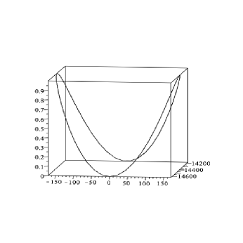
Figure 1. The second Veronese embedding of the circle of radius $1$ with center $(120,0)$.

(b) The invariant $\mu_{K}^{\ell}$ is invariant under rotations, but not under translations. For example if $K$ is the circle of radius $1$ in the plane centered at the point $(3,0)$. Then the second Veronese immersion of $K$ is given by

$$[0,2\pi]\ni t\mapsto\bigl{(}\,(3+\cos t)^{2},\sqrt{2}(3+\cos t)\sin t,\sin^{2}t\,\bigr{)}\in{\mathbb{R}}^{3}.$$

MAPLE aided computation shows that its pointwise curvature is

$$\kappa(t)=\sqrt{-{\frac{108\,\left(\cos\left(t\right)\right)^{3}-54\,\left(\cos\left(t\right)\right)^{2}-360\,\cos\left(t\right)-238}{-2\left(9\,\left(\cos\left(t\right)\right)^{2}-19-6\,\cos\left(t\right)\right)^{3}}}},$$

while its total curvature is

$$\mu_{K}^{2}\approx 2.065<2\sqrt{3\cdot 2-2}=4.$$

Numerical experimentation suggest that if $K(d)$ is the circle of radius $1$ centered at the point $(d,0)$ then

$$\lim_{d\rightarrow\infty}\mu^{2}_{K(d)}=2.$$

In view of Fenchel theorem, this would indicate that for $d$ large the second Veronese embedding of $K(d)$ is very close to a planar convex curve. The MAPLE generated Figure 1 seems to confirm this, since the second Veronese immersion is contained in a box of dimensions $1\times a\times b$, where $a>300$ and $b>400$. $\hbox to0.0pt{$\sqcap$\hss}\sqcup$

4. Critical points of trigonometric polynomials

As another application of Theorem 1.1, we want to compute the expected number of critical points on the unit circle of a trigonometric polynomial of degree $\leq n$.

Let $K$ denote the unit circle in ${\mathbb{R}}^{2}$ centered at the origin and denote by ${\boldsymbol{V}}_{n}$ the vector space of trigonometric polynomials of degree $\leq n$ on $K$, i.e., functions $f:K\rightarrow{\mathbb{R}}$ of the form

$$f(\theta)=a_{0}+\sum_{k=1}^{n}\bigl{(}\,a_{k}\cos k\theta+b_{k}\sin k\theta\,\bigr{)},$$

equipped with the inner product

$$(f,g)_{\boldsymbol{V}}=\frac{1}{2\pi}\int_{0}^{2\pi}f(\theta)g(\theta)d\theta.$$

Thus

$$\left|a_{0}+\sum_{k=1}^{n}\bigl{(}\,a_{k}\cos k\theta+b_{k}\sin k\theta\,\bigr{)}\,\right|^{2}_{\boldsymbol{V}}=a_{0}^{2}+\frac{1}{2}\sum_{k=1}^{n}(a_{k}^{2}+b_{k}^{2}).$$

We obtain an orthonormal basis of ${\boldsymbol{V}}_{n}$

$$\boldsymbol{e}_{0}=1,\;\;\boldsymbol{e}_{k}=\sqrt{2}\cos k\theta,\;\;\boldsymbol{f}_{k}=\sqrt{2}\sin k\theta,\;\;k=1,\dotsc,n.$$

The function

$$\xi:K\rightarrow{\boldsymbol{V}}_{n},\;\;[0,2\pi]\ni s\mapsto\xi_{s}^{\dagger}$$

defined by (1.2) +(1.3) is given in this case by the map

$$s\mapsto\xi_{s}^{\dagger}=\sqrt{2}\sum_{k=1}^{n}k\bigl{(}-(\sin ks)\boldsymbol{e}_{k}+(\cos ks)\boldsymbol{f}_{k}\,\bigr{)}.$$

Observe that

$$|\xi_{s}^{\dagger}|^{2}=2\sum_{k=1}^{n}k^{2}.$$

We set

$${\boldsymbol{\nu}}(s):=\frac{1}{|\xi_{s}^{\dagger}|}\xi_{s}^{\dagger}=\left(\sum_{k=1}^{n}k^{2}\right)^{-1/2}\sum_{k=1}^{n}k\bigl{(}-(\sin ks)\boldsymbol{e}_{k}+(\cos ks)\boldsymbol{f}_{k}\,\bigr{)}.$$

Then

$${\boldsymbol{\nu}}^{\prime}(s)=\left(\sum_{k=1}^{n}k^{2}\right)^{-1/2}\sum_{k=1}^{n}k^{2}\bigl{(}\,(\cos ks)\boldsymbol{e}_{k}-(\sin ks)\boldsymbol{f}_{k}\,\bigr{)},$$

so that

$$|{\boldsymbol{\nu}}^{\prime}(s)|=\left(\sum_{k=1}^{n}k^{2}\right)^{-1/2}\cdot\left(\sum_{k=1}^{n}k^{4}\right)^{1/2}$$

Using the classical identity

$$\sum_{k=1}^{n}k^{j}=\frac{1}{j+1}\beta_{j+1}(n+1),$$

where $\beta_{\ell}$ is the $\ell$-th Bernoulli polynomial we deduce

$$|{\boldsymbol{\nu}}^{\prime}(s)|=\sqrt{\frac{3\beta_{5}(n+1)}{5\beta_{3}(n+1)}},$$ (4.1)

where

$$\beta_{3}(x)=x^{3}-\frac{3}{2}x^{2}+\frac{1}{2}x,\;\;\beta_{5}(x)=x^{5}-\frac{5}{2}x^{4}+\frac{5}{3}x^{3}-\frac{1}{6}x.$$

The equality (4.1) and Theorem 1.1 imply the following result.

Theorem 4.1.

The expected number of critical points on the unit circle of a trigonometric polynomial of degree $\leq n$ is

$$T_{n}=2\sqrt{\frac{3\beta_{5}(n+1)}{5\beta_{3}(n+1)}}=2\sqrt{\frac{\sum_{k=1}^{n}k^{4}}{\sum_{k=1}^{n}k^{2}}}.$$

In particular

$$T_{n}\sim 2n\sqrt{\frac{3}{5}}\;\;\mbox{as $n\rightarrow\infty$}. \hbox to0.0pt{$\sqcap$\hss}\sqcup$$

Remark 4.2.

The above theorem indicates that for large $k$, a trigonometric polynomial of degree $k$ is expected to have approximately $2\sqrt{\frac{3}{5}}k\approx 1.549k$ critical points. In particular, it will likely have less that $2k$ critical points on the unit circle.

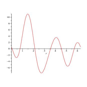
Figure 2. A “random” trigonometric polynomial of degree $4$.

In the MAPLE generated Figure 2 we depicted the graph of a “random” trigonometric polynomial of degree $4$

$$1.2\cos t+2.35\sin t-3.17\cos 2t+2.71\sin 2t+1.53\cos 3t-4.17\sin 3t$$

$$+\cos 4t-1.15\sin 4t.$$

We notice that it has $6$ critical points, which is very close to the expected value $T_{4}\approx 6.87$. $\hbox to0.0pt{$\sqcap$\hss}\sqcup$

References

- [1] S.S. Chern, R. Lashof: On the total curvature of immersed manifolds, Amer. J. Math., 79(1957), 306-318.
- [2] I. Fáry: Sur la courbure totale d’une courbe gauche faisant un noed, Bull. Soc. Math. France, 77(1949), 128-138.
- [3] H. Federer: Geometric Measure Theory, Springer Verlag, 1969.
- [4] S. G. Krantz, H.R. Parks: Geometric Integration Theory, Birkhäuser, 2008.
- [5] J.W. Milnor: On the total curvature of knots, Ann. Math., 52(1950), 248-257.
- [6] L.I. Nicolaescu: Lectures on the Geometry of Manifolds, 2nd Edition, World Scientific, 2007.
- [7] by same author: An Invitation to Morse Theory, Springer Verlag, 2007.