Optimisation of quantum Monte Carlo wave function: steepest descent method

Abstract

We have employed the steepest descent method to optimise the variational ground state quantum Monte Carlo wave function for He, Li, Be, B and C atoms. We have used both the direct energy minimisation and the variance minimisation approaches. Our calculations show that in spite of receiving insufficient attention, the steepest descent method can successfully minimise the wave function. All the derivatives of the trial wave function respect to spatial coordinates and variational parameters have been computed analytically. Our ground state energies are in a very good agreement with those obtained with diffusion quantum Monte Carlo method (DMC) and the exact results.

I Introduction

Quantum Monte Carlo (QMC) method has constituted an efficient and powerful numerical method for solving time-independent many-body Schrödinger equation mainly in chemistry and solid state physics hammond ; ceperley96 ; umrigar99 ; foulkes ; mcmillan ; ceperley77 ; fahy ; raghavachari ; needs ; neekamal . Among various approaches to QMC namely, random walk, diffusion, Green-function etc, variational quantum Monte Carlo (VMC) has been extensively studied in recent years foulkes . In VMC method, a parameterized many-body trial wave function is optimised according to Raleigh-Ritz variation principle. In practice, this task is done utilizing a numerical algorithm for optimisation the parameters. Various algorithms have been proposed and implemented in the framework of QMC such as Newton lin ; umrigar05 ; sorella05 , steepest descent (SD) huang90 ; huang96 ; huang99 , perturbative optimisation scemma ; toulouse and linear optimization method toulouse ; umrigar07 ; toulouse08 . The wave-function optimisation is implemented via two schemes namely energy minimisation and variance minimisation. These methods have their own merits and disadvantages. A basic task in VMC is the evaluation of first and second derivatives of the local energy $E_{L}=\frac{H\Psi}{\Psi}$ respect to variational parameters and spatial coordinates or a combination of them ($\Psi$ is the trial wave function). Despite normally the first derivative is analytically evaluated and the second derivatives are calculated numerically luchow there are papers in which second derivatives are also calculated analytically umrigar05 . Numerical evaluation of second derivatives causes a systematic error into the problem. To the best of our knowledge, the SD method has only been utilized in the variance minimisation approach huang96 . Our objective in this paper is to show that implementation of the SD method in the direct approach of energy minmisation yields reasonable results. We report our results for the ground state energies of He, Li, Be, B and C atoms and compare them to the results in the literature obtained by other methods.

II Variational wave function and steepest descent optimisation method

II.1 Theoretical background

Let us briefly explain the basic ingredients of the VMC method. In the VMC method a trial many-body wave function $\Psi(\vec{R},\{c_{m}\})$ containing a set of $M$ variational parameters $c_{1},c_{2},\cdots,c_{M}$ is considered. $\vec{R}$ denotes the position set of electrons. We confine ourselves to Born-Openheimer approximation in which the nuclei are assumed static and only the electronic degrees of freedom are taken into account. The parameters ${c_{m}}$ are varied according to the Raleigh-Ritz variation procedure so as to minimize the variational energy $E(\{c_{m}\})$ defined as follows:

$$E(\{c_{m}\})=\frac{\int\Psi^{*}(\vec{R},\{c_{m}\})H\Psi(\vec{R},\{c_{m}\})d\vec{R}}{\int\Psi^{*}(\vec{R},\{c_{m}\})\Psi(\vec{R},\{c_{m}\})d\vec{R}}$$ (1)

Where $H$ is the many body system Hamiltonian. We ignore relativistic correction and take the Hamiltonian as follows (in Hartree atomic units):

$$H=-\frac{1}{2}\sum_{i}\nabla_{i}^{2}-\sum_{i,I}\frac{Z_{I}}{r_{iI}}+\sum_{i<j}\frac{1}{r_{ij}}$$ (2)

Small letters refer to electrons and capital ones to nuclei. $Z_{I}$ is the electric charge of the $I$-th nucleus and $r_{ij}$ denotes the distance between electron $i$ and electron $j$ whereas $r_{iI}$ denotes the distance between electron $i$ and nucleus $I$. Moreover, we restrict ourselves to real-valued wave function $\Psi$ and omit the complex conjugate symbol afterwards. By introducing a local energy $E_{L}=\frac{H\Psi}{\Psi}$ and a normalized probability distribution function $p(\vec{R},\{c_{m}\})=\frac{\Psi^{2}(\vec{R},\{c_{m}\})}{\int\Psi^{2}(\vec{R},\{c_{m}\})d\vec{R}}$ We recast equation (1) in the following form:

$$E(\{c_{m}\})=\int p(\vec{R},\{c_{m}\})E_{L}d\vec{R}$$ (3)

It is now possible to approximate the integral by the standard Monte Carlo procedure:

$$E(\{c_{m}\})=lim_{N_{MC}\rightarrow\infty}\frac{1}{N_{MC}}\sum_{s=1}^{N_{MC}}E_{L,s}$$ (4)

$E_{L,s}$ denotes the local energy of the $s$-th sample of the configuration-space and $N_{MC}$ is the number of Monte Carlo sampling for evaluation of the integral.

II.2 Optimisation of the wave function: steepest descent method

The next step is to find the optimal values of the parameters which minimise the objective function i.e.; the variational energy $E$ sorella ; schautz ; toulouse . There exists numerous optimisation methods such as Newton lin ; umrigar05 ; myung , steepest descent huang90 ; huang96 ; huang99 , conjugate gradient etc in the literature. Here we focus on the simplest of them and show that despite simplicity algorithm is capable of exhibiting a satisfactory performance despite not receiving much attention. We briefly recall the main ingredient of this method. Having numerically computed the energy $E$ for a given set of parameters in (4), we iteratively update the values of the parameters according to the following procedure:

$${\bf c}^{k+1}={\bf c}^{k}-a{\bf g}^{k}$$ (5)

The vector ${\bf c}^{\dagger}=(c_{1},c_{2},\cdots,c_{M})$ denotes the parameters, $k$ is the iteration step and $a$ denotes the constant of the SD method. The vector ${\bf g}^{\dagger}=(\frac{\partial E}{\partial c_{1}},\frac{\partial E}{\partial c_{2}},\cdots,\frac{\partial E}{\partial c_{M}})$ is the gradient vector of energy respect to the parameters. We note that in some cases we should vary the SD constant in each iteration step to get the desired optimum value. In order to utilize SD method, we should evaluate the energy gradient vector. This has been done in details in lin . We only quote the result:

$$\frac{\partial E}{\partial c_{m}}=lim_{N_{MC}\rightarrow\infty}\frac{2}{N_{MC}}\sum_{s=1}^{N_{MC}}\{(\frac{\partial ln\Psi}{\partial c_{m}})_{s}(E_{L,s}-E)\}$$ (6)

In eq. (6) $(\frac{\partial ln\Psi}{\partial c_{m}})_{s}$ denotes the logarithmic derivative of wave function evaluated in the $s$-th MC configuration. If the constant $a$ is appropriately chosen the sequence ${\bf c}^{k}$ converges to ${\bf c}^{*}$ after some iterations.

II.3 Trial wave function and its parameters

We wish now to introduce the structure of the trial ground state wave function we have implemented in our calculations for simple atoms. We have taken the following well-known form for $\Psi$boys ; schmidt :

$$\Psi=D^{\uparrow}D^{\downarrow}e^{J}$$ (7)

In which $D^{\uparrow}$ and $D^{\downarrow}$ are up-spin and down-spin Slater determinants and $J$ is the Jastrow factor. The number of spatial orbitals $N_{up}(N_{down})$ in the construction of Slater determinant $D^{\uparrow}(D^{\downarrow})$ equals the number of spin up (down) electrons and depends on the atom we consider. Note that $N_{up}+N_{down}=N$ where $N$ is the number of electrons in the atom. For the basis set in the construction of up and down Slater determinants we have used a variant of Slater-type $s$ and $p$ orbital as follows garciaI ; garciaII :

$$\phi_{s}({\bf r})=\sum_{k=1}^{P}C_{k}e^{-\zeta_{k}r}+\sum_{k=1}^{P}C^{\prime}_{k}re^{-\zeta^{\prime}_{k}r}$$ (8)

$$\phi_{p_{x}}({\bf r})=\sum_{k=1}^{P}xD_{k}e^{-\xi_{k}r}$$ (9)

Analogous definitions goes for $p_{y}$ and $p_{z}$ orbitals. We have set $P=3$ in all our calculations. Henceforth, the parameters are $C_{k},C^{\prime}_{k},D_{k},\zeta_{k},\zeta^{\prime}_{k}$ and $\xi_{k}$ where $k=1,2,3$. For the Jastrow factor we have taken the following form:

$$J=\sum_{i<j}U_{ij}$$ (10)

The sum goes over all the particles (electrons) and $U_{ij}$ has the following dependence on distances:

$$U_{ij}=\sum_{mno}C_{mno}[(\frac{r_{i}}{1+r_{i}})^{m}(\frac{r_{j}}{1+r_{j}})^{n}+(\frac{r_{i}}{1+r_{i}})^{n}(\frac{r_{j}}{1+r_{j}})^{m}](\frac{r_{ij}}{1+r_{ij}})^{o}$$ (11)

$r_{i}$ is the distance between electron $i$ and the nucleus, $r_{ij}$ is the distance between electrons $i$ and $j$. Exponents $m,n,o$ are positive integers and the sum over $mno$ denotes the sum over given values of these integers. We adopt the following choice of integers schmidt $m,n,o$:

$$\{(0,0,1),(0,0,2),(0,0,3),(0,0,4),(2,0,0),(3,0,0),$$

$$(4,0,0),(2,2,2),(2,0,2)\}$$ (12)

Equation (11) includes electron-electron correlations (terms with $m=n=0$), electron-nucleus correlations ($o=0$ as well as one of $m$ or $n$ zero) and also electron-electron-nucleus correlations ((2,0,2) and (2,2,2) terms). Here we have considered the simplest choices compatible with electron-electron and electron-nucleus cusp conditions. The origin of three body correlation terms in (11) stems in the back flow correlation firstly suggested by Feynman and Cohen feynman . We refer the readers for more details to reference [25]. The Jastrow function has nine independent parameters $C_{mno}$. Each $s$ type orbital contains twelve parameters and in a $p$ orbital we have six parameters. We note that after imposing electron-nucleus cusp conditions, one parameter from each $s$ orbital will be fixed.

II.4 Variance minimisation method

In the preceding sections, we outlined the basics of energy minimisation method. In this method, we minimise the variational energy. In recent years, an alternative scheme the so-called variance minimisation has been introduced umrigar88 ; umrigar05 and has become one of the most frequently used method in the literature. This method has shown to provide some advantages over the straightforward energy minimisation. We now briefly review this method. Instead of energy, we minimise the variance of the local energy $E_{L}$ coldwell ; bartlett :

$$\sigma^{2}=\frac{\int\Psi^{2}(\vec{R},\{c_{m}\})(E_{L}-E)^{2}d\vec{R}}{\int\Psi^{2}(\vec{R},\{c_{m}\})d\vec{R}}=\langle(E_{L}-E)^{2}\rangle$$ (13)

All the other steps are analogous to those in the energy minimisation method. To implement the SD procedure we only should replace the energy gradient vector with the variance gradient vector. Derivatives of $\sigma^{2}$ respect to parameters have been evaluated in umrigar05 . Here for simplicity we use the following expression which ignores the change of the wave function umrigar05 :

$$\frac{\partial\sigma^{2}}{\partial c_{m}}=2\langle\frac{\partial E_{L}}{\partial c_{m}}(E_{L}-E)\rangle$$ (14)

More concisely the above approximation corresponds to underweighted variance minimisation method. The average is taken with the normalised probability function $p(\vec{R},\{c_{m}\})=\frac{\Psi^{2}(\vec{R},\{c_{m}\})}{\int\Psi^{2}(\vec{R},\{c_{m}\})d\vec{R}}$. We can approximate the average in (14) by a sum in MC approach. Note that when implementing this method, we have to replace $E$ with $\sigma^{2}$ in the gradient vector ${\bf g}^{\dagger}$ in equation (5). In the next section our results will be reported. All the computational details of the calculations are explained in the appendix.

III Application to atoms and discussion

We have implemented the steepest descent optimising method to find the ground state energy and wave function of atoms He, Li, Be, B and C by two approaches of energy and variance minimisation. Let us now explain our procedure of energy minimisation. It consists of three steps: anticipating the variational parameters, finding the optimised value of steepest descent parameter $a$ and eventually the fine tuning of variational energy. Step one begins with random initialization of the parameters values. Initial values of Jastrow parameters are randomly chosen in vicinity of zero. We then set the SD constant $a$ to a rather high value say $a=0.1$. Next we proceed with some iterations of (5) until the variational energy reaches approximately to the exact ground state energy. This comprises step one. During this step integrals in (1) are evaluated by the standard MC Metropolis method. Each MC move consists of a random selection of an electron and displace it from its position by the vector $\vec{\delta}$. The move size which is the length of $\vec{\delta}$ is randomly chosen (uniformly) from the interval $[0,\delta_{max}]$. The direction of $\vec{\delta}$ is uniformly chosen between zero and $2\pi$. We took the number of Monte Carlo steps $N_{MC}$ equal to $3\times 10^{5}$. We discard the first $10000$ steps to ensure reaching equilibrium. Averages are separated by $20$ MC steps to suppress the effects of correlations among generated MC configurations. The MC maximum move size $\delta_{max}$ has been typically $0.3$ (Hartree atomic units) with the acceptance ratio around $70$ percent. At the end of step one, which normally takes $5-6$ iterations, variational parameters should have reached to the vicinity of their ultimate values. We put their latest values in the code and re run it. This is the beginning of step two. We then proceed with some iterations until the iteration series of the variational energy begins to diverge. This shows that by the current value of the SD parameter we can no more reach the true energy. Here we reduce $a$ to a smaller value say one order of magnitude smaller and repeat the procedure until the iteration series of energy begins to diverge or strongly oscillates. We repeat this $a$ reduction procedure until further reduction of the SD constant $a$ does not lead to divergence of energy iteration series. Normally after $4-5$ repetitions we achieve our aim and $a$ reaches to a value of the order $10^{-5}$. This marks the end of step two and by now we have an iteration energy series. In figure (1) we have depicted such series of Be ground state energy obtained in the method explained above. Corresponding series for other atoms are similar in nature.

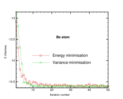
Figure 1: Ground state energy of Be in two methods of energy and variance minimisation.

It is seen that after roughly $20$ iterations we reach a steady state regime. Next in figure (2) we exhibit the dependence of absolute value of $\nabla_{c}E$ on the iteration number.

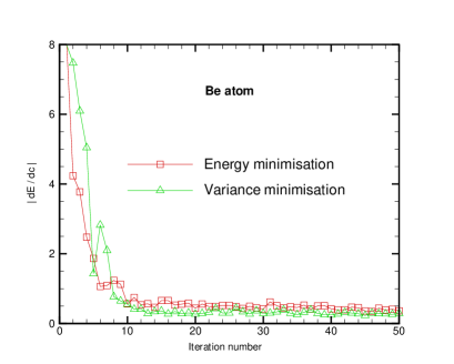
Figure 2: $|\nabla_{c}E|$ vs iteration number.

We see that $|\nabla_{{\bf c}}E|$ tends to a small value for a sufficient number of iterations. Theoretically it should goes to zero but due to numeric computations it does not approach to zero. Finally in third step, in which the fine tuning of energy in performed, we choose the variational parameters obtained from that iteration in the series which has the smallest energy and re run the code for these values of parameters for a longer MC run of $N_{MC}=2\times 10^{6}$ steps to find the energy in a fine tune manner. All the reported values in table I have been obtained in this way. In figure (3) the energy error is shown for both methods of energy and variance optimisation. We recall that the error has been obtained from the following formula:

$$error=\sqrt{\frac{\frac{1}{N_{MC}}\sum_{i=1}^{N_{MC}}[E_{L}(\vec{R_{i}})]^{2}-E^{2}}{N_{MC}-1}}$$ (15)

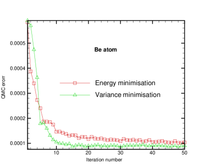
Figure 3: QMC error vs iteration number.

We see that the error is lower in variance minimisation method. In both methods, the error decreases as we increase the iteration number. In table I, we report the ground state energies we have obtained and compare them both to the existing computational results in the literature obtained by other methods lin ; schmidt ; casula and the exact ones chakravorty . The comparison shows that the steepest descent method is capable of minimising the energy to a very good precision. In fact our results by energy minimisation method is in most of the cases even better than those reported in schmidt ; lin . Besides Be, in all the atoms, our energy is comparable to the DMC energy. This marks the efficiency of the steepest descent method at least for light atoms. We should like to emphasize that simplicity is the main merit of our approach which can turn it into an efficient method al least for simple atoms. Our results obtained by variance minimisation method is less favourable in comparison to our energy minimisation ones. however, the error in the energy minimisation method is larger. Comparison of our variance minimisation results to those in lin (which have been obtained by VMC in Newton optimisation method ) shows that the results of lin is slightly better than ours. We have also compared our results to the recent paper of Brown et al brown in which besides single determinant, multideterminant trial wave function have been employed. It is seen that the accuracy of our results is comparable to those exhibited in brown .

IV Summary and Concluding Remarks

In summary we have applied the steepest descent optimisation method to optimise the parameters of the QMC many-body wave-function in some light atoms. Two schemes of energy and variance minimisation have been implemented. The key features to achieve the correct minimum is to vary the SD constant $a$ appropriately. Our results are in a well agreement with exact results and those obtained by DMC. We note that all the derivatives of the trial wave function respect to spatial coordinates and variational parameters have been analytically calculated.

Table 1: Variational energy with error bar for atoms He to C (All the energies are in Hartree).

	He	Li	Be	B	C
$E$(energy minimisation)	-2.9037(4)	-7.4780(4)	-14.648(1)	-24.640(9)	-37.831(8)
$E$(variance minimisation)	-2.9031(2)	-7.4757(3)	-14.6443(9)	-24.6244(3)	-37.807(5)
$E_{0}$(Refchakravorty )	-2.903719	-7.47806	-14.66736	-24.65391	-37.8450
$E_{VMC}$(Reflin )	-2.903717(8)	-7.47722(4)	-14.6475(1)	-24.6257(1)	-37.8116(2)
$E_{VMC}$(Refschmidt )	-2.9029(1)	-7.4731(6)	-14.6332(8)	-24.6113(8)	-37.7956(7)
$E_{DMC}$(Refcasula )	-2.903719	-7.4780(2)	-14.6565(4)	-24.63855(5)	-37.8296(8)
$E_{VMC}$(Refbrown )	no report	-7.47683(3)	-14.6311(1)	-24.6056(2)	-37.8147(1)

V acknowledgement

We highly appreciate very useful discussions with Mehdi Neek Amal. MEF is thankful to N. Arshado Do’leh for his useful helps.

VI Appendix

In this section we give some details of the manipulations for the evaluation of the integrals (3) and (14). In evaluation of these integrals, we have analytically calculated two basic quantities $E_{L},\frac{\partial ln\Psi}{\partial c_{m}}$ and $\frac{\partial E_{L}}{\partial c_{m}}$. Let us first consider $E_{L}$. According to its definition we have:

$$E_{L}=\frac{H\Psi}{\Psi}=-\frac{1}{2}\sum_{i}\frac{\nabla_{i}^{2}\psi}{\psi}+V$$ (16)

The first term is kinetic energy and $V$ represents the potential energy. Calculating $V$ is straightforward. To calculate the kinetic energy $KE$ we rewrite it in the following form kent :

$$KE=\sum_{i}-\frac{1}{2}[{\nabla_{i}^{2}\ln\Psi+(\overrightarrow{\nabla}_{i}\ln\Psi)^{2}}]$$ (17)

Concerning the form of the trail wave function, $\Psi=D^{\uparrow}D^{\downarrow}e^{J}$ we have:

$$\overrightarrow{\nabla}_{i}\ln\Psi=\frac{1}{D^{\uparrow}}\overrightarrow{\nabla}_{i}D^{\uparrow}+\frac{1}{D^{\downarrow}}\overrightarrow{\nabla}_{i}D^{\downarrow}+\overrightarrow{\nabla}_{i}J$$ (18)

and

$$\nabla_{i}^{2}\ln\Psi=-(\frac{1}{D^{\uparrow}}\overrightarrow{\nabla}_{i}D^{\uparrow})^{2}+\frac{1}{D^{\uparrow}}\nabla_{i}^{2}D^{\uparrow}-(\frac{1}{D^{\downarrow}}\overrightarrow{\nabla}_{i}D^{\downarrow})^{2}+$$

$$\frac{1}{D^{\downarrow}}\nabla_{i}^{2}D^{\downarrow}+\nabla_{i}^{2}J$$ (19)

We note that the entry $D_{ij}$ of any determinant $D$ equals $\phi_{i}({\bf r}_{j})$ in which the orbital $\phi_{i}$ is the $i$th orbital in the construction of D. To evaluate the matrix $\overrightarrow{\nabla}_{i}D$ we only have to replace the $i$th column of matrix D $C_{i}$ by a new column $\tilde{C}_{i}=(\overrightarrow{\nabla}_{i}\phi_{1}({\bf r}_{i}),\overrightarrow{\nabla}_{i}\phi_{2}({\bf r}_{i}),\cdots,\overrightarrow{\nabla}_{i}\phi_{N_{D}}({\bf r}_{N_{D}}))^{\dagger}$. The matrix $\nabla^{2}_{i}D$ is analogously constructed but with $\tilde{C}_{i}=(\nabla^{2}_{i}\phi_{1}({\bf r}_{i}),\nabla^{2}_{i}\phi_{2}({\bf r}_{i}),\cdots,\nabla^{2}_{i}\phi_{N_{D}}({\bf r}_{N_{D}}))^{\dagger}$. $N_{D}$ is the dimension of D.

The next quantity to evaluate is $\frac{\partial ln\Psi}{\partial c_{m}}$. Some straightforward calculations yields:

$$\frac{\partial\ln\Psi}{\partial c_{m}}=\frac{1}{D^{\uparrow}}\frac{\partial D^{\uparrow}}{\partial c_{m}}+\frac{1}{D^{\downarrow}}\frac{\partial D^{\downarrow}}{\partial c_{m}}+\frac{\partial J}{\partial c_{m}}$$ (20)

The derivative of a Slater determinant respect to $c_{m}$ equals a sum of $N_{D}$ determinants. The $i$th term of this sum is the determinant D with its $i$th column $C_{i}$ replaced with column $\tilde{C}_{i}=(\frac{\partial\phi_{1}({\bf r}_{i})}{\partial c_{m}},\frac{\partial\phi_{2}({\bf r}_{i})}{\partial c_{m}},\cdots,\frac{\partial\phi_{N_{D}}({\bf r}_{i})}{\partial c_{m}})^{\dagger}$.

Eventually in order to evaluate $\frac{\partial E_{L}}{\partial c_{m}}$ we proceed as follows (starting with (16)):

$$\frac{\partial E_{L}}{\partial c_{m}}=-\frac{1}{2}\sum_{i}\frac{\partial\nabla^{2}_{i}\ln\Psi}{\partial c_{m}}-\sum_{i}\overrightarrow{\nabla}_{i}\ln\Psi\cdot\frac{\partial\overrightarrow{\nabla}_{i}\ln\Psi}{\partial c_{m}}$$ (21)

The terms containing derivatives respect to $c_{m}$ can be evaluated as follows:

$$\frac{\partial\overrightarrow{\nabla}_{i}\ln\Psi}{\partial c_{m}}=-\frac{1}{(D^{\uparrow})^{2}}\frac{\partial D^{\uparrow}}{\partial c_{m}}\overrightarrow{\nabla}_{i}D^{\uparrow}+\frac{1}{D^{\uparrow}}\frac{\partial\overrightarrow{\nabla}_{i}D^{\uparrow}}{\partial c_{m}}-$$

$$\frac{1}{(D^{\downarrow})^{2}}\frac{\partial D^{\downarrow}}{\partial c_{m}}\overrightarrow{\nabla}_{i}D^{\downarrow}+\frac{1}{D^{\downarrow}}\frac{\partial\overrightarrow{\nabla}_{i}D^{\downarrow}}{\partial c_{m}}+\frac{\partial\overrightarrow{\nabla}_{i}J}{\partial c_{m}}$$ (22)

The second term gives the following expression:

$$\frac{\partial\nabla^{2}_{i}\ln\Psi}{\partial c_{m}}=\frac{2}{(D^{\uparrow})^{3}}\frac{\partial D^{\uparrow}}{\partial c_{m}}|\overrightarrow{\nabla}_{i}D^{\uparrow}|^{2}-\frac{2}{(D^{\uparrow})^{2}}\frac{\partial\overrightarrow{\nabla}_{i}D^{\uparrow}}{\partial c_{m}}\cdot\overrightarrow{\nabla}_{i}D^{\uparrow}$$

$$-\frac{1}{(D^{\uparrow})^{2}}\frac{\partial D^{\uparrow}}{\partial c_{m}}\cdot\nabla^{2}_{i}D^{\uparrow}+\frac{1}{D^{\uparrow}}\frac{\partial\nabla^{2}_{i}D^{\uparrow}}{\partial c_{m}}$$

$$+\frac{2}{(D^{\downarrow})^{3}}\frac{\partial D^{\downarrow}}{\partial c_{m}}|\overrightarrow{\nabla}_{i}D^{\downarrow}|^{2}-\frac{2}{(D^{\downarrow})^{2}}\frac{\partial\overrightarrow{\nabla}_{i}D^{\downarrow}}{\partial c_{m}}\cdot\overrightarrow{\nabla}_{i}D^{\downarrow}-$$

$$\frac{1}{(D^{\downarrow})^{2}}\frac{\partial D^{\downarrow}}{\partial c_{m}}\cdot\nabla^{2}_{i}D^{\downarrow}+\frac{1}{D^{\downarrow}}\frac{\partial\nabla^{2}_{i}D^{\downarrow}}{\partial c_{m}}+\frac{\partial\nabla^{2}_{i}J}{\partial c_{m}}$$ (23)

Note that in equations (22) and (23) to evaluate $\frac{\partial\nabla^{2}_{i}D}{\partial c_{m}}$ and $\frac{\partial\overrightarrow{\nabla}_{i}D}{\partial c_{m}}$ , we should first evaluate $\nabla^{2}_{i}D$ and $\overrightarrow{\nabla}_{i}D$ and then implement the derivatives respect to $c_{m}$.

References

- (1) B. L. Hammond, J. W. A. Lester and P. J. Reynolds, Monte Carlo Methods in Ab Initio Quantum Chemistry (World Scientific, Singapore,1994).
- (2) D. M. Ceperely and L. Mitas in, Advances in Chemical Physics, Vol XCIII, edited by I. Prigogine and S. A. Rice (John Wiley and Sons 1996).
- (3) Quantum Monte Carlo Methods in Physics and Chemistry , Eds. M. P. Nightingle and C. J. Umrigar, Nato ASI Ser. C 525, (Kluwer, Dordrecht, 1999).
- (4) W. M. C. Foulkes, L. Mitas, R. J. Needs and G. Rajagopal, Rev. Mod. Phys., 73 , 33 (2001).
- (5) W. L. McMillan, Phys. Rev. , 138, A442 (1965).
- (6) D. M. Ceperely and B. J. Alder, Phys. Rev. Lett., 45, 566 (1980).
- (7) S. Fahy, X. W. Wang and S. G. Louie, Phys. Rev. B., 42 , 3503 (1990).
- (8) K. Raghavachari and J. B. Anderson, J. Phys. Chem., 100 , 3703 (1996).
- (9) R. Maezono, A. Ma, M. D. Towler and R. J. Needs, Phys. Rev. Lett., 98, 025701 (2007).
- (10) M. Neekamal, G. Tayebirad, M. Molayem, M. E. Foulaadvand, L. Esmaleili-Sereshki and A. Namiranian, Solid state Communications, 145 ,594 (2008).
- (11) Xi Lin, H. Zhang, and A. M. Rappe, J. Chem. phys, 112, 2650 (2000).
- (12) C. J. Umrigar and C. Filippi, Phys. Rev. Lett., 94 , 150201 (2005).
- (13) S. Sorella, Phys. Rev. B, 71 , 241103 (2005).
- (14) S. Huang, Z. Sun, and W. A. Lester, Jr., J. Chem. Phys., 92 , 597 (1990).
- (15) H. Huang and Z. Cao, J. Chem. Phys., 104 , 200 (1996).
- (16) S. Huang, Q. Xie, Z. Cao, Z. Li, Z. Yue and L. Ming, J. Chem. Phys., 110 , 3703 (1999).
- (17) A. Scemma and C. Filippi, Phys. Rev. B, 73, 241101 (2006).
- (18) J. Toulouse and C. J. Umrigar, J. Chem. Phys., 126 , 084102 (2007).
- (19) C. J. Umrigar, J. Toulouse, C. Filippi, S. Sorella, R. G. Hennig, Phys. Rev. Let. 98, 110201 (2007);
- (20) J. Toulouse, C. J. Umrigar, J. Chem. Phys. 128, 174101 (2008).
- (21) A. Lüchow and J. B. Anderson, J. Chem. Phys., 105 , 7573 (1996).
- (22) S. Sorella, Phys. Rev. B., 64 , 024512 (2001).
- (23) F. Schautz and C. Filippi, J. Chem. Phys., 120 , 10931 (2004).
- (24) M. Won Lee, M. Mella, and A M. Rappe, J. Chem. Phys., 122 , 244103 (2005).
- (25) S. F. boys and N.C. Handy, Proc. R. Soc. London Ser. A, 310 , 63 (1969).
- (26) K. E. Schmidt and J. W. Moskowitz, J. Chem. Phys., 93 , 4172 (1990).
- (27) J. M. Garcia de la Vega and B. Miguel, Chem. Phys. Lett., 207 , 270 (1993).
- (28) J. M. Garcia de la Vega and B. Miguel, Int. J. Quantum Chem. , 51 ,397 (1994).
- (29) R. P. Feynman and M. Cohen, Phys. Rev., 102, 1189 (1956).
- (30) C. J. Umrigar, K. G. Wilson, and J. W. Wilkins, Phys. Rev. Lett., 60 , 1719 (1988).
- (31) R. L. Coldwell, Int. J. Quant. Chem., 11 , 215 (1977).
- (32) J. H. Bartlett, Phys. Rev. , 98 , 1067 (1955).
- (33) M. Casula and S. Sorella, J. Chem. Phys, 119, 6500 (2003).
- (34) S. J. Chakravorty, S. R. Gwaltney, E. R. Davidson, F. A. Parpia and C. F. Fishcer, Phys. Rev. A, 47, 3649 (1993).
- (35) P. R. C. Kent, PhD thesis, Cambridge university, (1999).
- (36) M. D. Brown, J. R. Trail, P.Lopez and R. J. Needs, J. Chem. Phys, 126, 224110 (2007).