A balanced homodyne detector for high-rate Gaussian-modulated coherent-state quantum key distribution

Abstract

We discuss excess noise contributions of a practical balanced homodyne detector in Gaussian-modulated coherent-state (GMCS) quantum key distribution (QKD). We point out the key generated from the original realistic model of GMCS QKD may not be secure. In our refined realistic model, we take into account excess noise due to the finite bandwidth of the homodyne detector and the fluctuation of the local oscillator. A high speed balanced homodyne detector suitable for GMCS QKD in the telecommunication wavelength region is built and experimentally tested. The 3 dB bandwidth of the balanced homodyne detector is found to be 104 MHz and its electronic noise level is 13 dB below the shot noise at a local oscillator level of 8.5$\times 10^{8}$ photon per pulse.

The secure key rate of a GMCS QKD experiment with this homodyne detector is expected to reach Mbits/s over a few kilometers.

I Introduction

Quantum key distribution (QKD) based on Gaussian-modulated coherent-state (GMCS) protocol has attracted a lot of attention Grosshans03 ; Namiki04 ; Lodewyck05 ; Legre06 ; Heid07 ; QiGMCS07 ; Lo08 . Comparing with the BB84 QKD, the GMCS QKD presents several advantages. The coherent state required by GMCS QKD can be produced easily by a practical laser source, while the perfect single photon source required by BB84 QKD is hard to obtain. Although improved BB84 protocols (such as decoy protocols Lo05 ; Ma05 ; Zhao05 ; Zhao06 ) are compatible with coherent laser sources, they do require single photon detectors, which are expensive and have low efficiency. The homodyne detector in the GMCS QKD, on the other hand, can be constructed using high efficiency PIN photodiodes Lodewyck05 . The GMCS QKD also has an advantage of transmitting multiple bits per symbol Grosshans03 ; Scarani08 . The security of the GMCS QKD was first proven against individual attacks with direct Grosshans02 or reverse Grosshans03 ; Grosshans04 reconciliation schemes. Security proofs were then given against general individual attacks Grosshans04 and general collective attacks Lodewyck07 ; Navascues06 ; GarciaPatron06 . To date, three groups have independently claimed that they have proved the unconditional security of GMCS QKD Renner08 ; Leverrier08 ; Zhaoyibo08 .

Fiber-based GMCS QKD systems over a practical distance are challenging and only a few groups have demonstrated QKD experiments over tens of kilometersLodewyck07 ; QiGMCS07 ; QiGMCS08 ; Fossier08 . Current repetition rates used in those GMCS QKD experiments are below 1 MHz, which in turn, makes the GMCS QKD less competitive than the single photon BB84 QKD operating at GHz repetition rates Dixon08 ; Zhang09 . The repetition rate of GMCS QKD is limited by a few factors: (1) the speed of the homodyne detector QiGMCS07 ; (2) the speed of the data acquisition system; and (3) the speed of the classical data processing algorithm Lodewyck05 . The speed of date acquisition and classical data processing can be increased by hardware engineering and are not fundamental limits in GMCS QKD. In this work, we mostly focus on increasing the homodyne detector speed and analyzing various excess noise contributions introduced by a practical homodyne detector.

The balanced homodyne detection used in quantum measurement, proposed by Yuen and Chan Yuen83 , plays an important role in quantum optics Slusher85 ; Brei97 ; Vasi00 and quantum cryptography Grosshans03 ; Lodewyck05 ; Lodewyck07 ; QiGMCS07 ; Fossier08 ; Xuan09 . In a balanced homodyne detector (BHD), the signal to be measured is mixed with a local oscillator (LO) at a beam splitter. The interference signals from the two output ports of the beam splitter are sent to two photodiodes followed by a subtraction operation, and then, amplification may be applied. The output of a BHD can be made to be proportional to either the amplitude quadrature or the phase quadrature of the input signal depending on the relative phase between the signal and the LO. The output of the BHD can be captured in either frequency Vasi98 or time domains Smithey93 ; Smithey99 ; Hansen01 ; Huisman09 . For GMCS QKD, measurement in the time domain that is capable of resolving each individual pulse (representing a weak coherent state) is required in order to extract random key information Grosshans03 . This pulse-resolving requirement demands that the bandwidth of the detection system be significantly higher than the repetition rate of the QKD operation, which highlights the importance of developing high bandwidth BHDs.

In this paper, we develop a broadband BHD suitable for GMCS QKD operating at a repetition rate of tens of MHz. To predict its performance in GMCS QKD, we first analyze the excess noise contributed by this practical BHD. In the GMCS QKD, excess noise is defined in units of shot noise and includes all noises due to system imperfections and eavesdropping, which are above and beyond the vacuum noise associated with channel loss and losses in Bob’s system. It determines the maximum amount of information that could be obtained by Eve. In the original realistic model proposed in previous GMCS QKD literature Grosshans03 ; Lodewyck07 ; QiGMCS07 , the excess noise contributed by a BHD is the electronic noise of the BHD. This model does not consider the excess noise that originates from other imperfections in a practical BHD and is not conservative enough in estimating the information possibly be leaked to Eve. In this paper, we refine the original realistic model which has been widely adopted to calculate key rates for practical GMCS QKD systems and identify two new noise sources of a practical homodyne detector: (1) the excess noise caused by the BHD electrical pulse overlap at the BHD output; and (2) the excess noise caused by LO fluctuation. Under the refined realistic model, we quantify the various excess noise contributions from the broadband BHD we constructed. Based on our simulation using the experimentally determined excess noise of the BHD, secure GMCS QKD key rates using this BHD is predicted to reach Mbits/s over a few kilometers.

This paper is organized as follows: In Section II, we revisit GMCS QKD protocol, identify two new excess noise sources, and introduce the key generation rate formulas based on the refined realistic model. In Section III, we analyze the excess noise contribution of a practical BHD. In Section IV, we discuss practical issues in building a high speed BHD, including different temporal responses of two photodiodes, appropriate pulse duration, and the BHD linearity and the construction of a high speed HD in GMCS QKD. In Section V, we will report the performance of the BHD and predict the key rates by simulation.

II Gaussian-modulated coherent-state protocol

The basic GMCS QKD protocol is as follows: Alice generates two random sets of continuous variables $x$ and $p$ with a Gaussian distribution that has a zero average. Alice encodes random bits (key information) by modulating the amplitude quadrature ($x$) and the phase quadrature ($p$) of weak coherent states $|{x+ip}\rangle$ (typically less than 100 photons in each pulse) with her Gaussian-distributed random variable sets $\{x,p\}$. On the receiver’s side, Bob measures either $x$ or $p$ quadrature of the weak coherent states randomly by using homodyne detection. By repeating this procedure multiple times, Alice shares a set of correlated Gaussian variables (called the “raw key”) with Bob. By comparing a random sample of their raw key, they can evaluate parameters of QKD and upper bound on Eve’s information. Finally, they can generate secure key by performing reconciliation.

In the presence of individual attacks, one can estimate the information leaked to Eve from the amount of excess noise quadrature noise observed by Bob in excess of standard quantum limit Grosshans03 . The most conservative estimation (the general model) assumes all the excess noise is introduced by eavesdropping, whereas the original realistic model assumes that Eve cannot control the LO or take advantage of the excess noise generated within Bob’s system Grosshans03 . In the original realistic model, the excess noise has several contributions: (1) noise due to imperfection outside Bob’s system is denoted as $\varepsilon_{A}$. This part of noise can be controlled by Eve; (2) noise from Bob’s system that is uncontrollable by Eve, called $N_{Bob}$. In Refs. Lodewyck05 ; Lodewyck07 , the latter refers to the homodyne detector noise ($N_{hom}$), while in Refs. QiGMCS07 ; QiGMCS08 , it consists both homodyne detector noise ($N_{hom}$) and the noise associated with the photon leakage from the LO to the signal ($N_{leak}$). In previous papers Lodewyck05 ; Lodewyck07 ; QiGMCS07 ; QiGMCS08 , $N_{hom}$ is regarded to consist of only the electronic noise (i.e. $N_{hom}$ = $N_{ele}$). In this paper, we refine this realistic model and consider other imperfections of a practical BHD, and conclude that excess noise caused by a practical BHD ($N_{hom}$) could be divided into three parts: (1) electronic noise ($N_{ele}$), (2) noise introduced by electrical pulse overlap due to finite response time of the BHD ($\varepsilon_{overlap}$) and (3) noise due to local oscillator fluctuation in the presence of incomplete subtraction of a BHD ($N_{LO}$).

In Ref. Lutkenhaus07 , the need to monitor the intensity of the LO for security proofs in discrete QKD protocol embedded in continuous variables has been discussed. In GMCS QKD experiment, Alice and Bob can monitor LO, and discard pulses with large intensity changes in LO. However, there is always a small measurement error due to imperfect measurement instrument. Therefore, it is reasonable to assume there is a small amount of LO fluctuation that Eve can take advantage of. Therefore, in this refined realistic model, $\varepsilon_{overlap}$ and $N_{LO}$ generated by a BHD, as well as $N_{leak}$ associated with leakage LO photons, are all considered controllable by Eve. $N_{LO}$ is caused by imperfect subtraction of BHD in the presence of LO intensity fluctuation while $N_{leak}$ is due to the interference between leakage photons and LO photons.

Following an approach similar to that in Grosshans03 , we will now present the GMCS QKD key rate formulas based on refined realistic model. The mutual information between Alice and Bob $I_{AB}$ is determined by the Shannon entropy Shannon48 . According to Refs. Grosshans03 ; Lodewyck05 ,

$$I_{AB}=\frac{1}{2}\log_{2}[(V+\chi)/(1+\chi)],$$ (1)

where

$$\chi=\chi_{vac}+\varepsilon=\frac{1-\eta G}{\eta G}+\varepsilon.$$ (2)

In Eq. (1), $V=V_{A}+1$ is the quadrature variance of the coherent state prepared by Alice (1 is the shot noise of a coherent state) and $V_{A}$ is Alice’s modulation variance (variance of $x$ or $p$ quadrature modulated by Alice). In Eqs. (1) and (2), $\chi$ is the equivalent noise measured at the input, which is composed of “vacuum noise” $\chi_{vac}$ (noise associated with the channel loss and detection efficiency of Bob’s system) and “excess noise” $\varepsilon$ (noise due to the imperfections in a non-ideal QKD system). $G$ is the channel efficiency (transmission), and $\eta$ is the total efficiency of Bob’s device (optical loss and detector efficiency).

We will now discuss the key rate formulas for the case of the refined realistic model, which we defined earlier in this Section. Under the refined realistic model, noise that can in principle be controlled by Eve ($\varepsilon_{E}$) includes (1) $\varepsilon_{A}$ due to imperfections outside Bob’s system; (2) $\varepsilon_{overlap}$ introduced by electrical pulse overlap due to finite response time of the BHD; (3) $N_{LO}$ due to LO fluctuations in the presence of incomplete subtraction of a BHD and (4) $N_{leak}$ associated with the leakage from LO to signal. Excess noise that is out of Eve’s control ($N_{Bob}$) is electronic noise from the homodyne detector ($N_{ele}$). Therefore, the total excess noise $\epsilon$ can be written as Grosshans03

$$\varepsilon=\varepsilon_{E}+N_{Bob}/\eta G,$$ (3)

where $\varepsilon_{E}=\varepsilon_{A}+\varepsilon_{overlap}+N_{LO}/\eta G+N_{leak}/\eta G$ and $N_{Bob}=N_{ele}$. $\varepsilon_{A}$ and $\varepsilon_{overlap}$ are referring to the input. $N_{LO}$, $N_{leak}$ and $N_{ele}$ are defined from the output and need to be divided by $\eta G$ when we convert them to the input. Figure 1 summarizes the various noise terms considered in the original realistic model and the refined realistic model. $N_{leak}$ is mostly determined by the design of the QKD system rather than by the BHD. Since our main goal is to study the excess noises contributed by the BHD, we simply assume $N_{leak}=0$ in this paper.

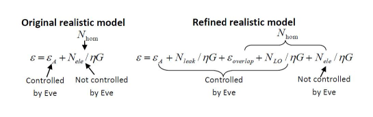
Figure 1: Various noise terms in the original realistic model and the refined realistic model.

From Eqs. (2) and (3), the equivalent input noise is

$$\chi=\frac{1-\eta G}{\eta G}+\varepsilon_{E}+\frac{N_{Bob}}{\eta G}.$$ (4)

With a reverse reconciliation scheme, the mutual information shared by Bob and Eve under the refined realistic model is

$$I_{BE}=\frac{1}{2}\log_{2}[\frac{\eta GV_{A}+1+\eta G\varepsilon}{\eta/{(1-G+G\varepsilon_{E}+GV^{-1})}+1-\eta+N_{Bob}}].$$ (5)

If a reverse reconciliation algorithm Grosshans03 is adopted, the secure key rate is

$$\Delta I=\beta I_{AB}-I_{BE}.$$ (6)

where $\beta$ is the reconciliation efficiency ($\beta\leq$ 1). In real QKD systems, $\beta$ is 0.9 in Ref. Fossier08 and 0.898 in Ref. Lodewyck07 . If the laser repetition rate of QKD experiment is $R$ Hz, the secure key per second can be written by

$$\Delta I_{second}=(\beta I_{AB}-I_{BE})\times R.$$ (7)

III Excess noise contributed by the BHD in a GMCS QKD

As previously stated, excess noise represents the amount of information that could possibly be leaked to Eve in a GMCS QKD system and is important in estimating the amount of secure information.

In this section, we will evaluate various sources of the excess noise for a practical BHD.

III.1 BHD electronic noise

Electronic noise $N_{ele}$ of a BHD is mainly contributed by thermal noise of electronic components and amplifier noise Bachor04 . Since shot noise scales with LO power and electronic noise is independent of the LO power Lvovsky08 , by measuring the BHD noise as a function of the LO power when vacuum is sent to the signal port, we can quantify the electronic noise in units of shot noise. Electronics noise in a BHD has been discussed in Appel07 .

III.2 Excess noise due to electrical pulse overlap

Ideally, the secure key rate of a GMCS QKD system is proportional to its operation rate. However, in practice, the BHD has a finite bandwidth. As the laser pulse repetition rate approaches the bandwidth of the BHD, we will expect a non-negligible overlap between adjacent electrical pulses at the output of the BHD. If the electrical pulses have overlap in the time domain, the measured quadrature value contains contributions from adjacent pulses.

We will estimate the amount of excess noise contributed by the electrical pulse overlap. The exact relation between the electrical pulse width $\tau$ and the BHD bandwidth $B$ depends on the electrical pulse shape. We have experimentally found that the relation $\tau\sim 1/B$ applicable to our homodyne detector. In this case, we can estimate the overlap by writing the following functions for two consecutive pulses: (a) $e^{-(t-1/R)^{2}/2\tau^{2}}$ and (b) $e^{-t^{2}/2\tau^{2}}$, where $R$ is the laser repetition rate and $\tau$ is the Gaussian pulse width. If the quadrature value is determined by the peak of the measured electrical pulse, the contribution of pulse (a) to pulse (b) is $e^{-\frac{B^{2}}{2R^{2}}}$. Since each pulse has two adjacent pulses, the excess noise contributed by electrical pulses overlap (referring to the input) is

$$\varepsilon_{overlap}=2V\times(e^{-\frac{B^{2}}{2R^{2}}})^{2}=2(V_{A}+1)\times e^{-\frac{B^{2}}{R^{2}}}.$$ (8)

where $V_{A}$ is Alice’s modulation. We remark that the excess noise due to the overlapping between adjacent pulses could be further reduced by deconvolution Huisman09 .

By decreasing this repetition rate, we can reduce the excess noise caused by overlap. However, the GMCS QKD key rate per second will be reduced too. In Fig. 2, we simulate the GMCS QKD key rate per second as a function of the repetition rate using Eqs. (1), (5), (6) and (7). With a BHD bandwidth of 100 MHz, the optimal pulse repetition rate is around 36 MHz. At repetition rates beyond $\sim$ 46 MHz, there will not be any secure key generated. At low repetition rate, the excess noise due to electrical pulse overlap is negligible compared to other excess noise contribution ($\varepsilon_{A}$), and the key rate per second is almost proportional to the repetition rate. As the repetition rate is increased beyond a critical point, the excess noise due to overlap is dominant and the key rate drops quickly with the repetition rate.

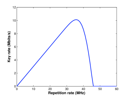
Figure 2: GMCS QKD secure key generation rate as a function of the laser repetition rate under the refined realistic model. The bandwidth of the BHD is 100 MHz. The simulation parameters are from Ref. QiGMCS07 , $V_{A}=16.9$, $G=0.758$, $\eta=0.44$, $\varepsilon_{A}$ = 0.056, $N_{ele}=0.045$, and $\beta$=0.898. In this simulation, $N_{LO}$ = $N_{leak}$ = 0.

III.3 Excess noise contributed by LO fluctuations

One of the advantages of BHD is that ideally the fluctuations of LO will be canceled after the subtraction. However, in a practical BHD, the positive and negative pulses cannot be canceled completely due to several reasons, such as different quantum efficiencies of the two photodiodes, different temporal responses of the photodiodes and the subsequent electronic amplifiers, or different optical intensities of the two balanced beams. The difference can be partially compensated, for example, by adjusting the losses and the relative delay of the two balanced arms, however, it cannot be completely canceled out. The remaining difference also varies with LO power. The consequence is that the fluctuation of the LO power will contribute to the excess noise.

The quadrature measurement corresponds to the time integrated electronic response of the detector. Neglecting the shot noise, this response equals

$$N_{LO}=I_{LO}[G_{1}t^{2}-G_{2}r^{2}],$$ (9)

where $I_{LO}$ is the number of photons in the local oscillator pulse, $t$ is the beam splitter transmittance, $r$ is reflectivity and $G_{1,2}$ are the time integrated gains of the amplifiers associated with the two photodiodes. We assumed that the quantum efficiency of the photodiodes is 1 and the signal is in the vacuum state. On the other hand, given that the variance in the number of photoelectrons in each photodiode due to the shot noise equals to the number of incident photons, we obtain the the output shot noise as

$$\langle N_{shot}^{2}\rangle=I_{LO}[G_{1}^{2}t^{2}+G_{2}^{2}r^{2}].$$ (10)

If the relative fluctuation of the LO power is $\sqrt{\langle\Delta I_{LO}^{2}\rangle}/I_{LO}=f$, the mean square fluctuation in the number of output photoelectrons in the units of shot noise is Raymer95

$$\frac{\langle\Delta N_{LO}^{2}\rangle}{\langle N_{shot}^{2}\rangle}=I_{LO}f^{2}\delta^{2}\quad\textrm{with}\quad\delta=\frac{G_{1}t^{2}-G_{2}r^{2}}{\sqrt{G_{1}^{2}t^{2}+G_{2}^{2}r^{2}}}.$$ (11)

For a well-balanced detector, $t^{2}\approx r^{2}\approx 1/2$ and $G_{1}\approx G_{2}$. In this case, the above expression can be written as $\delta\approx\delta_{opt}+\delta_{el}$, where $\delta_{opt}=t^{2}-r^{2}$ is the imbalance of the optical beam splitter whereas $\delta_{el}=(G_{1}-G_{2})/(G_{1}+G_{2})$ is the electronic characteristic of the balanced detector related to its common-mode rejection ratio (CMRR). In what follows, it is convenient to discuss $N_{LO}$ in terms of generalized CMRR which is measured in decibels and defined as

$$\rm{CMRR}=-20\log_{10}(2\delta).$$ (12)

The magnitude of $N_{LO}$ can be estimated from the Taylor decomposition of the noise variance as a function of the local oscillator power. The shot noise variance is proportional to the LO level, whereas $N_{LO}$ depends on it quadratically Bachor04 . We note that for determining $N_{LO}$, only time-integrated response functions (over the bandwidth of the homodyne detector) of the photodetector-amplifier systems are relevant; Faster-varying differences in the time dependent shapes of these functions play no role.

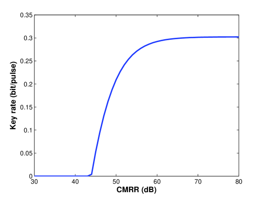
Figure 3: GMCS QKD secure key rate per pulse as a function of the CMRR using the refined realistic model. Here, we assume $10^{8}$ LO photons/pulse and 1 $\%$ LO fluctuation. The simulation parameters are from Ref. QiGMCS07 , $V_{A}=16.9$, $G=0.758$, $\eta=0.44$, $\varepsilon_{A}$ = 0.056, $N_{ele}=0.045$, and $\beta$=0.898. In this simulation, $\varepsilon_{overlap}$ = $N_{leak}$ = 0.

With the same GMCS QKD parameters used to produce Fig. 2, we simulate the GMCS QKD secure key rate as a function of the CMRR of the BHD in Fig. 3. When CMRR is lower than 55 dB (where key rate is 90 $\%$ of the maximum), key rate drops quickly as the CMRR drops. To obtain a positive key rate, the CMRR of the BHD should be greater than $\sim 44$ dB. When CMRR is greater than 55 dB, the secure key rate will not improve too much by increasing the CMRR since other excess noise contribution ($\varepsilon_{A}$) is dominant.

IV Construction and performance

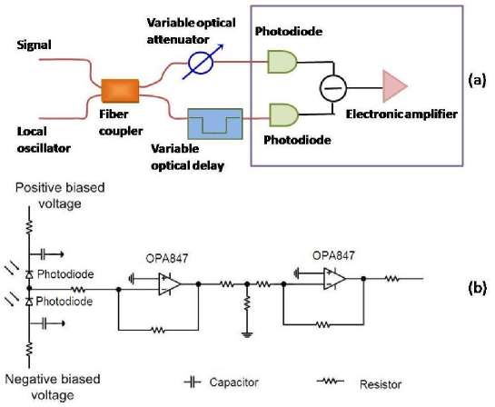
Figure 4: (a) Balanced homodyne detector (BHD) schematic in the telecommunication wavelength. The red lines are optical paths and the black lines are electrical cables. (b) Simplified BHD electronic circuit (the components in the right square of (a)).

In this section, we will present our construction and test results of a high speed BHD in the telecommunication wavelength region. We will also predict the excess noise and secure key rate by using this BHD in a GMCS QKD experiment.

IV.1 Schematic

Figure 4 (a) shows a schematic of our balanced homodyne detection system. In the telecommunication wavelength region, the signal and the LO beams will interfere at a two-by-two fiber coupler with a splitting ratio of 50:50. A variable optical attenuator and a variable optical delay are placed in the output paths of the fiber coupler, for adjusting losses and the lengths of the two paths accurately. Two photodiodes will detect the interference beams of the signal and the LO after precise balancing of time and intensity. Finally, a subtraction of the photocurrents generated by the two photodiodes is performed and the differential signal is amplified. To avoid disturbances from the environment, we used an enclosure to isolate the system of Fig. 4 (a).

In the electronic circuit shown in Fig. 4 (b), two InGaAs photodiodes from Thorlabs (FGA04, 2 GHz bandwidth, quantum efficiencies: 90 $\%$ and $93\%$) are reversely biased. The differential signal is amplified by two OPA847 operational amplifiers. The whole BHD circuit is built on a custom-designed printed circuit board. To minimize the parasitic capacitance, two photodiodes with short electrical contact legs are placed very close to each other.

IV.2 Linearity

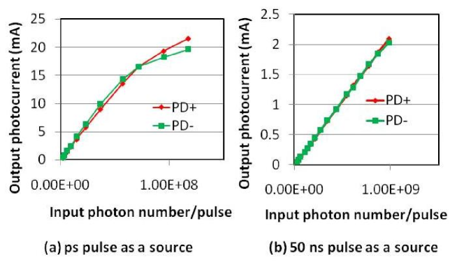
Figure 5: Photodiode linearity test. The peak photocurrent as a function of the input photon number in each pulse when (a) $\sim$ 1 ps width laser as a source; (b) 50 ns width laser as a source

In GMCS QKD, continuous Gaussian random numbers encoded on each pulse have to be recovered by the balanced homodyne detection on Bob’s side. To ensure the BHD output is proportional to the electric field quadrature of each pulse, the linearity of the BHD has to be guaranteed. In practice, the photodiode and electronic amplifiers can both have nonlinearities. A proper pulse width should be carefully chosen to guarantee that the photodiodes are working in their linear regions. In the test of the photodiode linearity, we send pulsed light to only one photodiode while blocking the other one. At a laser repetition rate of 10 MHz, we measure the output photocurrent generated by the photodiode (before it goes to the electronic amplifiers) at different incident optical powers using an oscilloscope. In Fig. 5, we compare the output electrical pulse peak current when a laser source with (a) $\sim$1 ps or (b) 50 ns pulse duration is used. We can see from Fig. 5 (a), the photodiodes saturate at a low optical input photon number per pulse than that of (b). In fact, the high peak power of the $\sim$1 ps-pulse ($\sim$ 18 W) saturates the photodiodes. In the case of 50-ns pulse as a source (Fig. 5 (b)), photodiodes are working in their linear regions (4 $\%$ deviation) up to $10^{9}$ photons/pulse.

The linearity test of the electronic amplifiers is shown in Fig. 6. By sending positive or negative electrical pulses (50-ns width, 10 MHz repetition rate) to the electrical amplifiers shown in Fig. 6 (a), we measure the output electrical pulse peak voltage as a function of the input electrical current. The trans-impedance gain is measured to be 22 kV/A in Fig. 6 (b). The trans-impedance gains for the positive and negative pulses are almost equal with less than 1 $\%$ deviation from their linear fits.

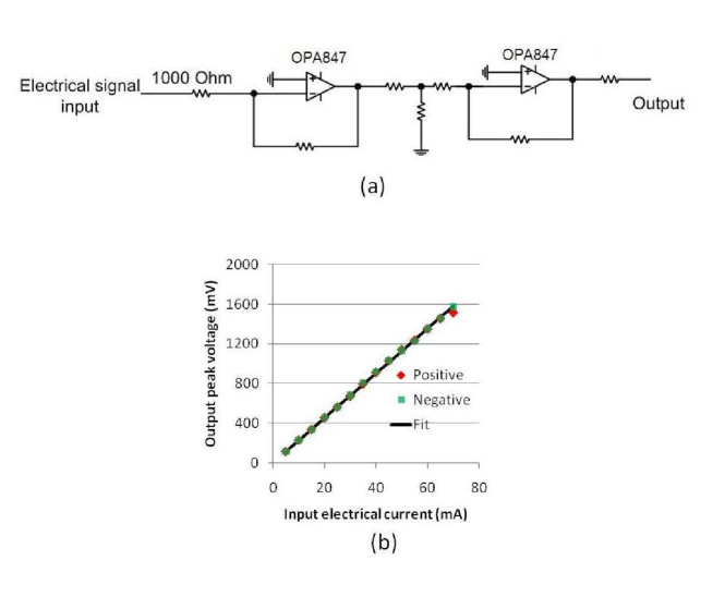
Figure 6: (a) Electronic amplifier linearity test circuit; (b) Output electrical pulse peak voltage as a function of input electrical current.

IV.3 BHD bandwidth

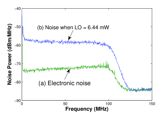
Figure 7: (a) Electronic noise (b) BHD noise at an LO of 6.44 mW.

We first characterize the bandwidth of our BHD by sending a CW LO. In this case, the residual signal caused by different temporal responses of the photodiodes can be eliminated by adjusting the loss in one arm (Fig. 4 a). Using an RF spectrum analyzer, the spectral noise is measured and shown in Fig. 7. In the frequency domain, the trace (a) is the electronic noise and is measured when no optical signal is sent to the BHD. We can see the 3-dB bandwidth of the BHD is 104 MHz. Trace (b) is measured when 6.64 mW CW LO is sent to the BHD. The noise includes electronic noise and shot noise.

IV.4 Homodyne detector noise measurement in the time domain

In GMCS QKD, each pulse will be measured individually. In the time domain, we first performed HD noise measurement at a pulse repetition rate of 10 MHz and obtained 12 dB shot noise to electronic noise ratio at an LO photon level of 8.2 $\times 10^{8}$. We further increase the repetition rate to 32 MHz and will demonstrate our results here.

With a 16-ns-width pulsed LO (5-ns edge time) at a repetition rate of 32 MHz, the total noise of BHD of each pulse is obtained by integrating the BHD output voltage over the pulse region. With an oscilloscope sampling rate of 20 G samples/s, and an integration time window of 20 ns in each cycle, each pulse quadrature is obtained from 400 sample points. Noise variance is obtained from 640 pulses. Fig. 8 shows the BHD noise variance as a function of the LO photon number per pulse. The measured homodyne detector noise includes: (1) electronics noise $N_{ele}$, (2) shot noise, and (3) noise associated with LO fluctuation $N_{LO}$. Because Fig. 8 displays the square variance, the shot noise should appear linear to the LO level, and $N_{LO}$, which is linear to LO level in shot-noise units becomes quadratically dependent on LO level when plotted in V² units. Note that $\varepsilon_{overlap}$ is neglected since it is much less than the shot noise when the signal is vacuum. We distinguish noises by separating the quadratic LO-dependent ($N_{LO}$), the linear LO-dependent (shot noise) and LO-independent ($N_{ele}$) components of the BHD output signal. From the experimental results, the total variance of the BHD output signal (in V²)can be written as $y=8.0\times 10^{-20}\cdot I_{LO}^{2}+7.0\times 10^{-10}\cdot I_{LO}+0.028$ where $I_{LO}$ is the LO photon number per pulse. The coefficient of determination is 0.999 Notefitting . The electronic noise $N_{ele}$ (in shot noise unit) can be determined from the ratio of the third term and the second term, which is 4.0$\times 10^{7}/I_{LO}$. We find the shot noise to electronic noise ratio is 13 dB at an LO photon level of $8.5\times 10^{8}$ per pulse. In the meantime, $N_{LO}$ (in shot noise unit) can be determined from the ratio of the first term to the second term, which is $1.1\times 10^{-10}\times I_{LO}$.

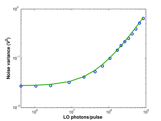
Figure 8: Total noise of BHD as a function of the LO photon number per pulse.

As a simple check of the randomness of the noise, we measure the correlation coefficient (CC) between adjacent sampling results. CC is defined as

$${\rm CC}=\frac{{E(X(n)X(n+1))}-E(X(n))E(X(n+1))}{\sqrt{E(X(n)^{2})-E^{2}(X(n))}\sqrt{E(X(n+1)^{2})-E^{2}(X(n+1))}}.$$ (13)

while $X(n)$ is the quadrature value of the $n$th pulse. At 3.4$\times 10^{8}$ LO photons/pulse, the correlation coefficient between consecutive pulses is 0.051, which is comparable with other BHDs reported in Ref. Okubo08 (0.04) and Ref. Haderka09 (0.07). We can use the CC to determine the upper bound of the excess noise caused by electrical pulse overlap $\varepsilon_{overlap}$. In GMCS QKD, with the quadrature variance of the coherent state prepared by Alice $V$, the excess noise due to the overlap between pulses will be $V\times{\rm CC}^{2}=(V_{A}+1)\times\rm{CC}^{2}$ (referring to the input) Explain4 . Assuming Alice’s modulation $V_{A}$ = 16.9 QiGMCS07 and each pulse has two neighboring pulses, we derive the excess noise caused by BHD pulse overlap to be 0.044 referring to the input.

IV.5 Common mode rejection ratio

To quantify the subtraction capability of the BHD, we measure the CMRR. In the frequency domain, we obtain CMRR by measuring the spectral power difference at the repetition rate of 32 MHz in two cases: (a) one photodiode is blocked and the other is illuminated (b) both photodiodes are illuminated. At an LO power of 24.6 $\mu$W, the spectral noise for both cases is shown in Fig. 9. The CMRR is obtained to be 46.0 dB.

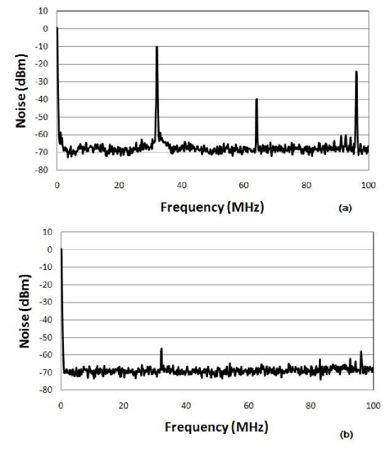
Figure 9: Noise spectrum at an LO power of 24.6 $\mu$W when (a)two photodiodes are illuminated; (b)one photodiode is blocked. Resolution bandwidth: 100 kHz

IV.6 Excess noise evaluation and key rate simulation for a GMCS QKD experiment

Table 1: Excess noise contributions by the BHD (in the shot noise unit). $I_{LO}$ indicates the LO photon number per pulse.

	Referring to the input			Referring to the output
$N_{ele}$	$4.0\times 10^{7}/(\eta GI_{LO})$			$4.0\times 10^{7}/I_{LO}$
$\varepsilon_{overlap}$	0.044			0.044$\times\eta G$
$N_{LO}$	$1.1\times 10^{-10}\cdot I_{LO}/\eta G$			$1.1\times 10^{-10}\cdot I_{LO}$

Under this refined realistic model, we identify new excess noise sources of a practical BHD. Various sources of excess noise contributed by this BHD are summarized in Table 1. Given this practical BHD, we can also optimize operation parameters based on the refined realistic model. In Fig. 10, we simulate the key rate per pulse as a function of the LO level. The key rate under the refined realistic model will reach the maximum at an LO photon number of $1.3\times 10^{8}$ per pulse, because there is a tradeoff between $N_{LO}$ (increasing with LO level) and $N_{ele}$ (decreasing with LO level).

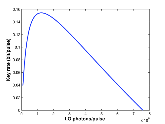
Figure 10: Optimization of LO photon number under the refined realistic model. The simulation parameters are from Table 1 and Ref. QiGMCS07 , $G=0.758$, $V_{A}=16.9$, $\eta=0.44$, $\varepsilon_{A}$ = 0.056, and $\beta$=0.898.

In Fig. 11, we simulate the secure key rate of GMCS QKD using this BHD under the refined realistic model by choosing the optimal LO level for each transmittance. With this high speed BHD allowing a repetition rate of tens of MHz, the secure key generation rate of GMCS QKD can be improved by 1-2 orders of magnitude comparing to current systems at 500 kHz repetition rate in Ref. Lodewyck07 (with a key rate of 2 kbits/s over 25 km fiber), and in Ref. Fossier08 (with a key rate of 8 kbits/s over 3 dB loss channel) and at 100 kHz in Ref. QiGMCS08 (with a key rate of 5 kbits/s over 20 km fiber). From the key rate simulation in Fig. 11, we expect to achieve a few Mbits/s over a short distance in future GMCS QKD under the refined realistic model.

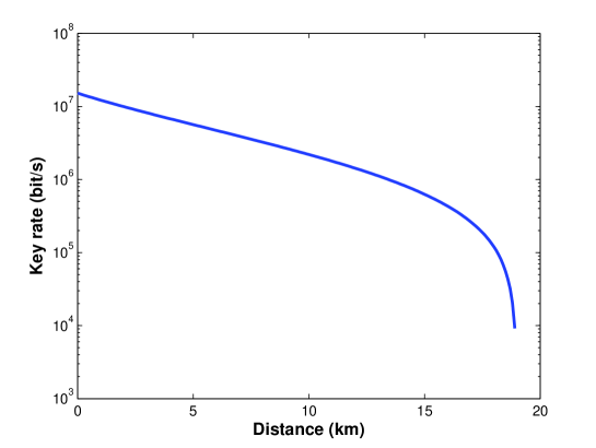
Figure 11: QKD secure key rate under the refined realistic model as a function of the transmission distance when the repetition rate is 32 MHz based on the performance of our BHD. The simulation parameters are from Table 1 and Ref. QiGMCS07 , $V_{A}=16.9$, $\eta=0.44$, $\varepsilon_{A}$ = 0.056, and $\beta$=0.898. Fiber loss is 0.21 dB/km. For each distance, the LO level is chosen to maximize the secure key rate. No secure key rate can be generated beyond 20 km due to the excess noise.

V Conclusion

In conclusion, we have analyzed the excess noise contributed by a practical BHD and refined the realistic model. The electronic noise $N_{ele}$, excess noise due to electrical pulse overlap $\varepsilon_{overlap}$ and excess noise caused by LO fluctuations in the presence of incomplete subtraction $N_{LO}$ are three excess noise sources for a practical BHD. They introduce a security loophole since Eve can monitor the pulse width and slightly change the LO intensity. Implementing attacks with current technology to GMCS QKD will be an interesting research direction to explore.

We also developed a high speed BHD with a 104 MHz bandwidth in the telecommunication wavelength region for the first time. A comparison of the specifications between our BHD and other high speed BHD is shown in Table 2. We achieved a shot-noise-to-electronic-noise ratio of 13 dB in the time domain at a pulse repetition rate of 32 MHz. The BHD has a high CMRR of 46.0 dB. Various sources of excess noise introduced by this practical BHD are identified, and their contributions to excess noise are evaluated. With this BHD, the key generation rate of GMCS QKD experiments is expected to reach a few Mbits/s under the refined realistic model.

Table 2: A comparison between high speed BHD

	Okubo08	Haderka09	Zavatta02	Our BHD
Wavelength (nm)	1064	800	786	1550
Bandwidth (MHz)	$\sim$ 250	$\sim$ 70	$\geq$ 82	$\sim$ 100
CMRR (dB)	45	61.8	42	46.0
Shot-noise-to-electronic-noise ratio (dB)	7.5	12	-	13

VI Acknowledgement

We thank CFI, CIPI, the CRC program, CIFAR, MITACS, NSERC, OIT, and QuantumWorks for their financial support.

References

- (1) F. Grosshsans, G. Van Assche, J. Wenger, R. Brouri, N. Cerf and P. Grangier, Nature 421, 238 (2003).
- (2) R. Namiki and T. Hirano, Phys. Rev. Lett., 92, 117901 (2004).
- (3) J. Lodewyck, T. Debuisschert, R. Tualle-Brouri, and P. Grangier, Phys. Rev. A 72, 050303 (R) (2005).
- (4) M. Legr, H. Zbinden and N. Gisin, Quant. Inf. and Comp., 6, 324 (2006).
- (5) M. Heid and N. Lutkenhaus, Phys. Rev. A, 76, 022313 (2007).
- (6) B. Qi, L.-L.Huang, L. Qian and H.-K. Lo, Phys. Rev. A 76, 052323 (2007).
- (7) H. -K. Lo and Y. Zhao, Encyclopedia of Complexity and System Science 8, 7265 (2009).
- (8) W.-Y. Hwang, Phys. Rev. Lett. 91, 057901 (2003); H.-K. Lo, in Proceedings of IEEE ISIT 2004, p. 137; H.-K. Lo, X. Ma, K. Chen, Phys. Rev. Lett. 94 230504 (2005); X. -B. Wang, Phys. Rev. Lett. 94 230503 (2005).
- (9) X. Ma, B. Qi, Y. Zhao, H.-K. Lo, Phys. Rev. A 72 012326 (2005); X. B. Wang, Phys. Rev. A 72, 012322 (2005).
- (10) Y. Zhao, B. Qi, X. Ma, H.-K. Lo, L. Qian,Phys. Rev. Lett. 96 070502 (2006).
- (11) Y. Zhao, B. Qi, X. Ma, H.-K. Lo, and L. Qian, in Proceedings of IEEE International Symposium on Information Theory (IEEE, 2006), pp. 2094-2098.
- (12) V. Scarani, H. Bechmann-Pasquinucci, N. J. Cerf, M. Dusek, N. Lutkenhaus, and M. Peev, Rev. Mod. Phys. 81, 1301 (2009).
- (13) F. Grosshans and P. Grangier, Phys. Rev. Lett., 88, 057902 (2002).
- (14) F. Grosshans and N. J. Cerf, Phys. Rev. Lett., 92, 047905 (2004).
- (15) J. Lodewyck, M. Bloch, R. Garc a-Patr n, S. Fossier, E. Karpov, E. Diamanti, T. Debuisschert, N. J. Cerf, R. Tualle-Brouri, S. W. McLaughlin, and P. Grangier, Phys. Rev. A 76, 042305 (2007).
- (16) M. Navascues and F. Grosshans and A. Acin, Phys. Rev. Lett. 97, 190502 (2006).
- (17) R. Garcia-Patron and N. J. Cerf, Phys. Rev. Lett. 97, 190503 (2006).
- (18) R. Renner and J. I. Cirac, Phys. Rev. Lett. 102, 110504 (2009), (2008).
- (19) A. Leverrier, E. Karpov, P. Grangier, and N. J. Cerf, New J. Phys., 11, 115009 (2009).
- (20) Y.-B. Zhao, Z.-F. Han and G.-C. Guo, arXiv:0809.2683v2 (2008).
- (21) B. Qi, L.-L. Huang, Y.-M. Chi, L. Qian and H. -K. Lo, in oral presentation at CELO/QELS 2008, paper QWE1; B. Qi, L.-L. Huang, Y.-M. Chi, L. Qian and H. -K. Lo, in SPIE Optics + Photonics 2008 San Diego, CA, Aug. 10-14, 2008.
- (22) S. Fossier, E. Diamanti, T. Debuisschert, A. Villing, R. Tualle-Brouri, and P. Grangier, New J. Phys. 11, 045023 (2009).
- (23) Q. D. Xuan, Z. Zhang, and P. L. Voss, Opt. Exp., 17, 24244 (2009).
- (24) A. R. Dixon, Z. L. Yuan, J. F. Dynes, A. W. Sharpe,and A. J. Shields, Opt. Express 16, 18790 (2008).
- (25) Q. Zhang, H. Takesue, T. Honjo, K. Wen, T. Hirohata, M. Suyama, Y. Takiguchi, H. Kamada, Y. Tokura, O. Tadanaga, Y. Nishida, M. Asobe, and Y. Yamamoto, New J. Phys. 11, 045010 (2009).
- (26) H. P. Yuen and V. W. S. Chan, Opt. Lett. 8, 177 (1983).
- (27) R. E. Slusher, L. W. Hollberg, B. Yurke, J. C. Mertz, and J. F. Valley, Phys. Rev. Lett. 55, 2409 (1985).
- (28) G. Breitenbach, S. Scheiller, and J. Mlynek, Nature 387, 471 (1997).
- (29) M. Vasilyev, S. -K. Choi, P. Kumar, and G. M. D’Ariano, Phys. Rev. Lett. 84, 2354 (2000).
- (30) M. Vasilyev, S.-K. Choi, P. Kumar, and G. M. D’Ariano, Opt. Lett. 23, 1393 (1998).
- (31) D. T. Smithey, M. Beck, M. G. Raymer, and A. Faridani, Phys. Rev. Lett. 70, 1244 (1993).
- (32) D. T. Smithey, M. Beck, M. Belsley, and M. G. Raymer, Phys. Rev. Lett. 69, 2650 (1999).
- (33) H. Hansen, T. Aichele, C. Hettich, P. Lodahl, A. I. Lvovsky, J. Mlynek and S. Schiller, Opt. Lett. 26, 1430 (2001).
- (34) S. R. Huisman, Nitin Jain, S. A. Babichev, Frank Vewinger, A. N. Zhang, S. H. Youn, and A. I. Lvovsky, Opt. Lett. 34, 2739 (2009).
- (35) C. Shannon, Bell Syst. Tech. J. 27, 379 (1948).
- (36) H. Bachor and T. C. Ralph, A guide to experiment in Quantum optics (Wiley-VCH, 2004).
- (37) A. I. Lvovsky and M. G. Raymer, Reviews of Modern Physics 81, 299 (2009).
- (38) J. Appel, D. Hoffman, E. Figueroa and A. I. Lvovsky, Physical Review A 75, 035802 (2007).
- (39) M. G. Raymer, J. Cooper, H. J. Carmichael, M. Beck and D. T. Smithey, J. Opt. Soc. Am. B 12, 1801 (1995).
- (40) Hauke Hseler, Tobias Moroder, and Norbert Ltkenhaus, Phys. Rev. A 77, 032303 (2008).
- (41) R. Okubo, M. Hirano, Y. Zhang and T. Hirano, Opt. Lett. 33, 1458 (2008).
- (42) O. Haderka, V. Michalek, V. Urbasek, and M. Jezek, Appl. Opt. 48, 2884 (2009).
- (43) If the measured HD noise is represented by and the fitting noise is represented by while is the index for each LO level, the coefficient of determination is determined by .
- (44) Assuming we have a long sequence of pulse quadrature values measured by a BHD, if we consider is contributed by the ()th, th, th pulses, we can write the pulse quadrature to be ( is a small number). The correlation coefficient (CC) between consecutive pulses is CC = . If we assume (only consecutive pulse value has a non-zero expectation), CC = . In GMCS QKD, the variance of Bob’s measurement of individual pulse will be contributed by the variances of its adjacent pulses. With the quadrature modulation of the coherent state prepared by Alice , the excess noise due to the overlap between pulses referring to the input will be .
- (45) A. Zavatta, M. Bellini, P. L. Ramazza, F. Marin, and F. T. Arecchi, J. Opt. Soc. Am. B 19, 1189 (2002).