Sub-systems in nearby solar-type wide binaries

Abstract

We conducted a deep survey of resolved sub-systems among wide binaries with solar-type components within 67 pc from the Sun. Images of 61 stars in the $K$ and $H$ bands were obtained with the NICI adaptive-optics instrument on the 8-m Gemini-South telescope. Our maximum detectable magnitude difference is about $5^{m}$ and $7.8^{m}$ at $0.15^{\prime\prime}$ and $0.9^{\prime\prime}$ separations, respectively. This enables a complete census of sub-systems with stellar companions in the projected separation range from 5 to 100 AU. Out of 7 such companions found in our sample, only one was known previously. We determine that the fraction of sub-systems with projected separations above 5 AU is $0.12\pm 0.04$ and that the distribution of their mass ratio is flat, with a power-law index $0.2\pm 0.5$. Comparing this with the properties of closer spectroscopic sub-systems (separations below 1 AU), it appears that the mass-ratio distribution does not depend on the separation. The frequency of sub-systems in the separation ranges below 1 AU and between 5 and 100 AU is similar, about 0.15. Unbiased statistics of multiplicity higher than two, advanced by this work, provide constraints on star-formation theory.

1 Introduction

The quest for exo-planets has attracted attention to stars in the solar neighbourhood. A complete understanding of their formation requires a quantitative and predictive description of stellar multiplicity. Empirical data on stellar multiplicity serve as a benchmark for star formation theories, for example to compare with recent large-scale hydrodynamical simulations (Bate, 2009). Although multiplicity statistics of solar-type dwarfs were assumed to be known since the survey of Duquennoy & Mayor (1991), in fact that survey did not constrain multiplicities higher than two because (i) the sample of 164 stars was too small and (ii) the discovery of wide binaries relied on traditional visual techniques. Raghavan (2009) shows that Duquennoy & Mayor (1991) missed half of higher-order multiples within 25 pc from the Sun.

Several studies of large samples of nearby stars are now in progress. Radial-velocity (RV) techniques ensure a secure detection of all short-period stellar companions (see summary in Grether & Lineweaver, 2006). However, for wider separations ($>$ 10 AU) RV variations are too slow or too small, and such companions are better discovered by direct imaging. Several recent deep imaging surveys, summarized by Metchev & Hillenbrandt (2009), aimed to detect substellar or planetary-mass companions to nearby stars, obtaining statistics of stellar companions as a by-product. The typical sample size of imaging surveys is still small, on the order of 100 targets.

Most imaging and RV surveys for low-mass companions explicitly avoid known visual binaries (e.g. Chauvin et al., 2010), so important star-formation effects may not be represented in their samples. For example, catalogued triples show that the mass-ratio distributions in close inner sub-systems discovered spectroscopically and in wider “visual” sub-systems are radically different (see Section 5). One of our goals is to investigate if this is a selection effect or a genuine feature of the star-formation process.

In order to improve the multiplicity statistics of a well-defined and sufficiently large distance-limited sample, we focus on $\sim$5000 dwarfs with $0.5<V-I<0.8$ within 67 pc from the Sun. According to preliminary estimates, there should be some 400 triples and 100 quadruples in this sample. Surveying such a large sample to detect those multiples with a reasonably deep and known completeness limit is a large task; here we address only a small part of it. Instead of avoiding known binaries, we purposefuly selected wide visual binaries from this sample. Some of these targets are also monitored in RV, giving complementary constraints on sub-systems with short periods (Desidera et al., 2006).

We imaged the chosen wide binaries with Adaptive Optics (AO) to study the properties of inner sub-systems. AO imaging on 8-m class telescopes provides nearly diffraction-limited resolution of 0.06^′′ in the near-infrared, which corresponds to a projected orbital radius of 4 AU for the farthest target stars in our sample, filling an important gap between RV and seeing-limited imaging surveys.

Our sample is detailed in Section 2. Observations, data reduction, and detection limits are described in Section 3, the results are presented in Section 4. Sections 5 and 6 contain the discussion and conclusions, respectively.

2 The sample of wide binaries

The wide binaries chosen for our survey belong to a large sample of nearby solar-type dwarfs (Nsample) selected from the latest version of Hipparcos catalog (van Leeuwen, 2007) by the following criteria:

1. trigonometric parallax $\pi_{\rm HIP}<15$ mas (within 67 pc from the Sun, distance modulus $<4.12^{m}$);

2. color $0.5<V-I<0.8$ (this corresponds approximately to spectral types from F5V to K0V);

3. unevolved, satisfying the condition $M_{\rm Hp}>9(V-I)-3.5$, where $M_{\rm Hp}$ is the absolute magnitude in the Hipparcos band calculated with $\pi_{\rm HIP}$.

There are 5040 stars (i.e. Hipparcos catalog entries) satisfying these conditions. Some of these stars with erroneous parallaxes or colors will be eventually removed from the sample, but this contamination is expected to be minor. The Nsample defined above is reasonably complete because the cumulative object count versus distance $d$ follows the $d^{3}$ law, deviating from it by only 10% at $d=67$ pc.

Visual binaries with separations $5^{\prime\prime}<\rho<20^{\prime\prime}$ and one or both components belonging to the Nsample were selected for AO observations from the Washington Double-Star Catalog, WDS (Mason et al., 2001). Additionally, we require each pair to have at least 3 observations and magnitudes of both components listed in the WDS, and that apparent motion of the wide pair be compatible with $\pi_{\rm HIP}$. As most targets have large proper motions, relative stability of the binary position over time permits rejection of optical pairs. An additional check was made by placing the components on the $(M_{V},V-K)$ color-magnitude diagram (CMD). There are $\sim$200 wide binaries in this list, 101 with negative declinations.

Table 1: Data on observed targets

HIP (A/B)	$\pi_{\rm HIP}$	$\rho$	$r$	Component A			Component B			Date	Rem
	mas	′′	AU	$V$	$H$	$K_{s}$	$V$	$H$	$K_{s}$	2000+
2028/29	24.0	16.5	687	8.39	7.46	7.41	9.56	8.30	8.27	09.9400	B
10579	17.2	6.7	390	9.43	8.06	7.97	9.97	8.34	8.24	09.9400
20552	36.1	5.6	155	6.87	5.37	5.32	7.23	5.64	5.55	10.0851
20610/12	16.7	10.5	629	8.06	6.89	6.84	8.27	7.01	6.98	10.0851	B
21963	18.2	8.2	450	8.13	6.69	6.62	13.30	8.99	8.75	10.0852
22531/34	26.0	12.9	496	5.61	4.88	4.80	6.24	5.28	5.19	09.9404	A,CRN
23926/23	18.7	10.1	540	6.83	5.20	5.10	10.29	8.00	7.90	10.0851
24711/12	15.3	13.3	867	8.46	7.00	6.95	10.57	8.29	8.24	10.0852
27922	42.4	10.4	246	7.60	5.84	5.76	10.57	7.40	7.22	10.0852
28790	37.2	5.6	150	6.02	4.92	4.75	8.98	6.09	6.03	10.0853
30158	17.8	7.0	390	8.57	7.02	6.91	10.58	8.09	8.03	10.0853
32644	21.2	4.9	230	7.37	6.05	5.97	8.66	6.61	6.52	10.0852
36165/60	31.2	17.7	566	7.08	5.92	5.80	8.06	6.75	6.60	10.0854
37332/33	15.1	15.7	1043	7.89	6.47	6.41	10.01	8.35	8.25	10.0855
37335	21.8	6.1	282	8.93	7.05	6.99	12.38	8.59	8.40	10.0855
39409	15.7	5.1	328	9.26	7.57	7.44	9.36	7.56	7.43	10.0855
43947	26.6	10.2	383	8.44	7.28	7.19	9.95	8.27	8.20	10.0857
44584/85	17.0	10.5	617	8.09	6.99	6.90	9.19	7.72	7.70	10.0857	B
44804	15.5	7.4	478	8.80	7.20	7.15	10.70	8.45	8.29	10.0857
45734	17.6	9.0	513	8.41	6.85	6.78	9.66	7.56	7.44	10.0856
45940	28.6	6.8	237	8.17	6.55	6.43	11.86	8.35	8.07	10.0856
46236	21.4	19.3	900	7.03	5.77	5.69	10.18	7.82	7.68	10.0856
47839/36	40.2	18.8	468	8.08	6.79	6.70	8.23	6.99	6.85	10.0858
49520	16.9	9.6	565	8. 82	7.35	7.24	8.99	7.40	7.30	10.0858
50638/36	83.3	17.1	205	7.67	5.18	4.98	9.67	8.46	8.40	10.0858
50883	16.2	6.7	413	7.90	6.71	6.62	13.00	9.05	8.98	10.0858
55288	20.8	9.5	456	7.10	5.91	5.82	7.91	6.32	6.22	10.0859
58240/41	21.1	18.9	895	7.67	6.24	6.13	7.83	6.29	6.24	10.0859
59021	19.4	6.0	308	6.69	5.24	5.10	8.84	6.71	6.55	10.0859	CRN
61595	17.8	8.4	472	8.28	6.80	6.68	10.48	8.29	8.12	10.0860	A
64498	18.0	9.3	516	7.74	6.40	6.25	10.10	7.98	7.85	10.0861
65176	17.8	5.0	282	7.85	6.47	6.40	8.59	6.82	6.68	10.0861
67408	33.9	11.6	342	6.62	5.29	5.22	10.21	7.14	7.02	10.0860	A,CRN

In Table 1 we list basic data on the components of the 33 wide pairs observed in this run. Column 1 gives the Hipparcos numbers of the primary and, in some cases, secondary components. The next three columns contain $\pi_{\rm HIP}$, binary separation $\rho$, and projected separation $r=\rho/\pi_{\rm HIP}$. Then follow the magnitudes of the primary (A) and secondary (B) components in the $V$, $H$, and $K_{s}$ bands as listed in the WDS and 2MASS (Cutri et al., 2003). The last two columns contain the date of observations and remarks where we indicate 5 cases when only one component was observed and 3 cases when the coronagraphic mask was used.

3 Observations and data reduction

3.1 Observing procedure

The Near-Infrared Coronagraphic Imager, NICI, on the Gemini South telescope is an 85-element curvature AO instrument based on natural guide stars (Toomey & Ftaclas, 2003; Chun et al., 2008). We used NICI in normal (non-coronagraphic) mode, as a classical AO system. However, simultaneous imaging in the two infrared bands $H$ and $K$ offered by NICI helps to distinguish faint companions from static speckles (the radial distance of a static speckle scales with wavelength while the position of a real detection does not change). The two detectors have $1024^{2}$ pixels of 18 mas (milliarcseconds) size, covering a square field of $18^{\prime\prime}$.

To avoid saturation, we used narrow-band filters with central wavelengths 2.272 $\mu$m and 1.587 $\mu$m in the red and blue channels, respectively. The minimum possible exposure time is 0.38 s, still causing saturation for bright targets. We observed three of the brightest stars with the coronagraphic mask of $0.32^{\prime\prime}$ radius, using in this instance broadband $K$ and $H$ filters. For the remaining bright targets we allowed moderate saturation. As the tradeoff between slower observations with more complex data reduction in coronagraphic mode and slightly saturated PSFs is not obvious, we tried both.

Typically, each target was observed at 5–6 dithered positions for a total accumulation time of about 5 min. The dither offsets were designed to take images of both wide-binary components in one frame whenever possible ($\rho<10^{\prime\prime}$) while closing the AO loop on the primary. Components of wider pairs were observed separately, except secondaries with $V>12^{m}$, too faint to serve as AO guide stars.

Of the two nights allocated to this program, one was lost due to a technical problem. Three targets were observed on 2009 December 10 in service mode. The remaining objects were observed on the night of 2010 January 31 to February 1 in classical mode. The seeing during that night was good. As measured from the NICI AO loop data, it ranged between $0.34^{\prime\prime}$ and $0.94^{\prime\prime}$, with a median of $0.50^{\prime\prime}$ (at 500 nm, not corrected to the zenith). High AO performance was achieved (see next Section). The transparency was variable (light cirrus). Out of 202 binary components accessible to NICI, we were able to observe 61, or 30%. The efficiency was high, with an average of 12 min per target including telescope slew, tuning of the primary mirror, acquisition of the object on the science camera, closing the AO loop, and data-taking.

3.2 Data processing

The data were processed in a standard way using custom IDL programs. Individual images written to separate FITS files were combined into data cubes, separately in red and blue channels. The sky image was obtained for each target as a median of the cube, then subtracted from each plane of the cube. After correcting for bad pixels and dividing by the flat field, the images were re-centered by cross-correlation and median-combined.

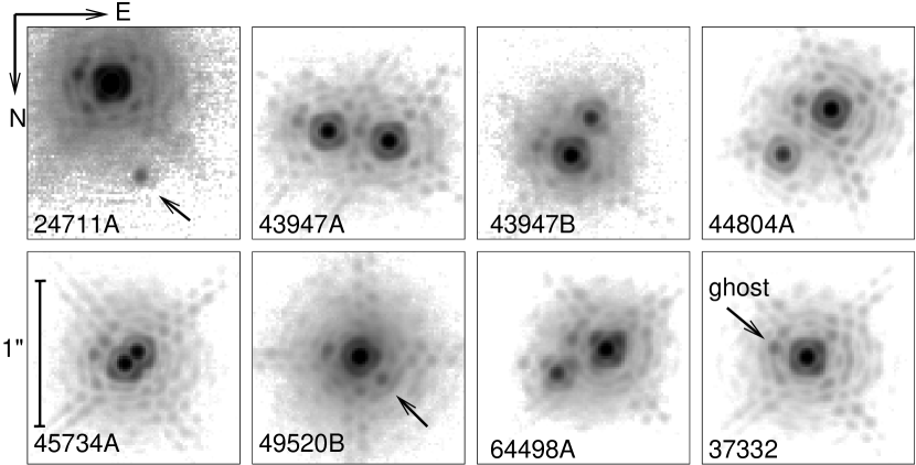
Figure 1: Mosaic of resolved-component images in the r-channel, labeled by the Hipparcos numbers. Each frame is 81 pixels ($1.46^{\prime\prime}$) across, oriented North down and East to the right. The intensity scaling is negative logarithmic. The first 7 frames show all binary components where we detected a close companion. The last frame shows the PSF of the unresolved target HIP 37332, with the ghost marked. The faint companions to HIP 24711A and HIP 49520B are marked by arrows. Note that at good AO correction the typical features of the NICI PSF become visible. These are particularly the double diffraction spikes and the four spots on the first Airy ring, giving it a “boxy” look. These features are caused by the oversized vanes of a spider mask placed in the pupil plane to control scatter.

Most frames contain just one or two bright point sources corresponding to the components of the wide binary. The position of each point source was recorded by “clicking” on its image, then refined by fitting a 2-dimensional Gaussian to the central part of the Point Spread Function (PSF) within 5-pixel radius. The ratio of the central intensity of this Gaussian to the total flux in a $0.9^{\prime\prime}$ diameter circle gives an estimate of the Strehl ratio. The typical Strehls are 43% and 22% in the red and blue channel, respectively, with maximum values reaching 54% and 38%. The median Full Width at Half Maximum (FWHM) of the PSF core was 65 mas and 57 mas in the red and blue channels, respectively. The diffraction limit $\lambda/D$ is 63 mas and 44 mas for the effective aperture diameter $D=7.5$ m set by the coronagraphic mask.

Figure 1 shows the mosaic of 7 close sub-systems found around some primary components of wide binaries. Most companions are rather obvious, well above the detection threshold. The PSFs contain also a faint secondary reflex at 13 pixels ($0.24^{\prime\prime}$), with a magnitude difference in the red channel of about $4.3^{m}$. This ghost (illustrated in Fig. 1 in the case of HIP 37332) is detected in all targets, and can be taken advantage of as a fiducial (see Section 3.4). Its position is the same in both channels, whereas the static speckle pattern scales in proportion to the wavelength.

3.3 Measurement of binaries

To measure the relative position and flux ratio of wide binaries more precisely, we fit the scaled and shifted image of the primary component (A) to the secondary (B). Such fits work very well, leaving only small residuals, and produce mutually consistent measurements in the two channels. The rms scatter between the wide-binary positions measured in two NICI channels is 5.5 mas in both radial and tangential directions.

We checked the pixel scale and detector orientation by comparing the measured positions of 16 wide pairs (the widest in Table 2 after exclusion of HIP 21963, 43947 and 50883, which were not used) with the positions listed in the Hipparcos Double and Multiple Star Catalogue (ESA, 1997). We did not find any systematic effect above noise and therefore used the nominal pixel scale of 18.0 mas for both channels. We found that the detector orientation of the channels differs by $1.01^{\circ}\pm 0.01^{\circ}$, so $1.0^{\circ}$ were added to measured angles in the blue channel.

For close pairs where the PSFs overlap, we use a variant of iterative blind deconvolution. Good preliminary estimates of the relative component’s position and intensity are already available from the Gaussian fits of the PSF cores. The image Fourier Transform (FT) is divided by the FT of the binary with preliminary parameters to get an estimate of the PSF. Negative parts of this PSF are set to zero and it is replaced by its azimuthal average at radial distances over 5 pixels from the center. The binary parameters are refined by fitting again the image with this synthetic PSF. Then the process is repeated, obtaining a second approximation to the PSF and using it again (without azimuthal averaging) to obtain the final binary parameters. The success of this procedure is verified by inspecting the resulting PSF, which should be “clean,” with the least possible trace of the companion.

3.4 Detection limits

Figure 2: Estimated $5\sigma$ companion detection limit (solid line) in the red channel for HIP 37332. The simulated companions are over-plotted as asterisks (detected) or empty squares (missed). The dotted line shows the 2-segment model.

To determine detection limits, we use mostly the data from the red NICI channel where the detection of low-mass components is deeper because of the smaller magnitude difference and larger Strehl ratios. The maximum magnitude difference of detectable companions $\Delta m_{\rm lim}$ is estimated by calculating the rms flux variations $\sigma(\rho)$ in circular zones of increasing radii $\rho$ centered on the main component. It is assumed that a detectable companion will have maximum intensity exceeding $5\sigma$, therefore

$$\Delta m_{\rm lim}(\rho)<-2.5\log_{10}[5\sigma(\rho)/I_{\rm max}].$$ (1)

This assumption is, of course, simplistic. We do not account for the existence of two simultaneous images in red and blue channels and for the good knowledge of the PSF from other companions of the same target or from other targets observed shortly before or after. Nevertheless, this simple strategy of estimating detection limits is sufficient for our purpose and has been tried before with good results (e.g. Tokovinin et al., 2006).

The limits computed for HIP 37322 are shown in Fig. 2. A bump is produced in the curves at $\rho\approx 13$ pixels by the ghost and by fixed speckle pattern (see the PSF in Fig. 1). To confirm the validity of (1), we performed Monte-Carlo simulations, adding artificial companions within $\pm 1.5^{m}$ from the estimated $\Delta m_{\rm lim}$. Secure detection of the ghost ($\Delta m=4.3$, $\rho=0.24^{\prime\prime}$) in all images gives confidence in our estimation of $\Delta m_{\rm lim}$.

The $5\sigma$ detection limits $\Delta m_{\rm lim}(\rho)$ were fitted by two straight lines intersecting at $\rho=8$ pixels ($0.144^{\prime\prime}$). The second segment extends from 8 to 50 pixels ($0.9^{\prime\prime}$), but the region between 8 and 16 pixel radius affected by the ghost and strong speckle is avoided in the fit. At $\rho>50$ pixels $\Delta m_{\rm lim}$ is assumed to be constant. Only two numbers $\Delta m(8)$ and $\Delta m(50)$ adequately describe the actual $\Delta m_{\rm lim}(\rho)$ curves, with typical rms error of only $0.3^{m}$ (excluding the zone between 8 and 16 pixel radii where the $5\sigma$ method does not properly account for the static speckle).

Detection limits were determined by the above procedure for all targets, although the Monte Carlo simulation checks were only performed for a subset. The two detection parameters $\Delta m(8)$ and $\Delta m(50)$ vary little between targets. Their median values are 5.02 and 7.79, respectively; the quartiles are (4.29, 5.22) and (7.03, 8.06). In the following we apply median detection parameters to all targets, including the three coronagraphic images where the actual limits should be deeper.

The detection limits found here match other similar studies done with “standard” AO. For example, companion detection was complete down to $\Delta K<3.9$ at $0.14^{\prime\prime}$ and $\Delta K<7.9$ at $0.9^{\prime\prime}$ in (Tokovinin et al., 2006). Similar results were obtained by Eggenberger et al. (2007). The deep companion survey at Palomar and Keck conducted by Metchev & Hillenbrandt (2009) also reached $\Delta K<8$ at $0.9^{\prime\prime}$. Note that typical detection limits with NICI are much deeper for dedicated planet search programs. In these cases long exposure times and techniques such as angular and spectral differential imaging are applied (Biller et al., 2008; Artigau et al., 2008).

4 Results

Table 2: Measured parameters of known and new pairs

HIP	Comp	Red channel (2.272 $\mu$m)			Blue channel (1.587 $\mu$m)			Rem
		$\theta$	$\rho$	$\Delta m$	$\theta$	$\rho$	$\Delta m$
		∘	′′	mag	∘	′′	mag
10579	A,B	288.58	6.710	0.47	288.50	6.703	0.71
20552	A,B	247.35	5.405	0.16	247.55	5.403	0.26	sat?
21963	A,B	92.33	8.184	2.35	92.26	8.169	2.64
23926	A,B	259.93	10.255	2.35	259.96	10.246	2.66	sat
24711	Aa,Ab	17.70	0.670	5.28	17.71	0.663	5.66	new
24711	B,C	324.85	11.135	6.29	324.87	11.132	6.45	opt
27922	A,B	19.35	10.742	1.55	19.37	10.727	1.88
28790	A,B	215.28	5.945	1.29	215.18	5.941	1.48	sat
30158	A,B	7.48	7.096	1.18	7.38	7.093	1.33
32644	A,B	160.49	5.029	0.72	160.43	5.039	0.73	sat?
37735	A,B	128.43	6.210	1.57	128.49	6.200	1.76
39409	A,B	329.64	5.187	0.10	329.67	5.193	0.14
43652	A,Ca	128.47	9.206	6.16	128.48	9.188	6.41	opt
43652	Ca,Cb	328.86	0.124	0.67	330.90	0.126	0.64	opt
43947	Aa,Ab	260.79	0.424	0.31	260.78	0.423	0.30	new
43947	Ba,Bb	152.16	0.289	1.65	152.16	0.289	1.73	new
43947	Aa,Ba	202.89	10.377	0.82	202.78	10.365	0.90
44804	Aa,B	136.01	7.175	1.16	136.08	7.167	1.21
44804	Aa,Ab	313.09	0.453	1.84	313.09	0.452	2.02	new
45734	Aa,Ab	132.69	0.119	0.38	133.33	0.117	0.36
45734	Aa,B	193.63	9.077	0.71	193.65	9.076	1.23
45940	A,B	69.28	6.713	1.72	69.29	6.705	1.98
47836	A,C	328.29	9.809	5.31	328.36	9.797	5.77	opt
49520	A,B	326.95	9.552	0.29	326.95	9.543	0.44
49520	Ba,Bb	44.21	0.213	3.61	46.69	0.210	3.40	new
50883	A,B	192.65	6.839	2.33	192.57	6.830	2.57
50883	A,C	299.87	7.379	6.23	299.82	7.363	6.55	opt
55288	A,B	253.94	9.462	0.54	253.96	9.456	0.84
58241	A,C	118.32	4.015	6.38	118.09	4.008	6.52
64498	Aa,B	302.20	9.464	1.59	302.24	9.458	1.91
64498	Aa,Ab	296.55	0.372	1.76	296.31	0.370	2.01	new
65176	A,B	96.89	5.168	0.61	96.95	5.164	0.62

4.1 Companion data

We have found 6 new close companions, one previously known companion, and several faint optical companions (Fig. 1). Table 2 lists the relative positions and magnitude differences in known and new pairs. Each pair is identified by the HIP number and component designations. The measured position angles in degrees, separations in arcseconds, and magnitude differences are listed separately for the two NICI channels.

The large rms difference between Hipparcos and our measurements of the wide pairs (130 mas in $\rho$ and $1.05^{\circ}$ in $\theta$) is mostly caused by their motion between the two epochs. The comparison with the relative positions of the same binaries deduced from the 2MASS Point Source Catalog (Cutri et al., 2003) has confirmed that no systematic corrections are needed and has shown a scatter of similar magnitude.

Remarks in the last column of Table 2 indicate cases when the image was saturated (the relative photometry may be compromised), newly detected close companions, and likely optical companions. These faint companions with separations of a few arcseconds would be dynamically unstable within wide binaries, should they be physical.

4.2 Notes on individual systems

HIP 28790 has a common-proper-motion companion C at $196^{\prime\prime}$.

HIP 36165 A is suspected to be a spectroscopic binary (SB).

HIP 43947 is unexpectedly discovered to be a resolved quadruple system. Both components are located $\sim 2^{m}$ below the Main Sequence in the $(M_{V},V-K)$ CMD, possibly because the Hipparcos parallax measurement was biased by the motions in the sub-systems. The position and $\Delta m$ of the wide pair Aa,Ba is derived from the Gaussian fits, therefore it may be less accurate.

HIP 45734: This is a young pre-Main-sequence system and X-ray source RX J0919.4-7738. It projects on the Chamaeleon star-forming region, but is located much closer than the corresponding association. Covino et al. (1997) found from a single spectrum that component B (southern) is a double-lined SB, with a large RV difference from A (see also Desidera et al., 2006). A itself is a close visual binary KOH83 resolved in March 1996 by Köhler (2001). He measured the position $(173.9^{\circ},0.109^{\prime\prime})$ and $\Delta K=0.45$. This is the only previously known resolved sub-system among the observed stars. Follow-up observations will soon lead to the visual orbit and mass measurement, adding another empirical point to the evolutionary tracks of young stars.

HIP 49520: The faint companion Bb is close to the detection limit (see Fig. 1). Yet, it is securely detected in both channels and stands up clearly in residuals when fitting the image of B with the image of A.

HIP 50638/36: The wide pair has been observed since 1835; it is definitely physical. Component B is variable. For this reason, probably, it is located on the CMD some $6^{m}$ below the MS, while A is on the MS with the parallax $\pi_{\rm HIP}=83$ mas listed in Table 1. According to van Leeuwen (2007), the parallaxes and proper motions of the two components are discordant, but have large errors. Future RV measurements can settle the controversy.

HIP 59021: Component A is a suspected SB and also an astrometric binary (acceleration solution in Hipparcos). Non-detection of the sub-system with NICI means that its period is likely less than 10 y, or it is a white dwarf.

4.3 Estimation of the mass ratios

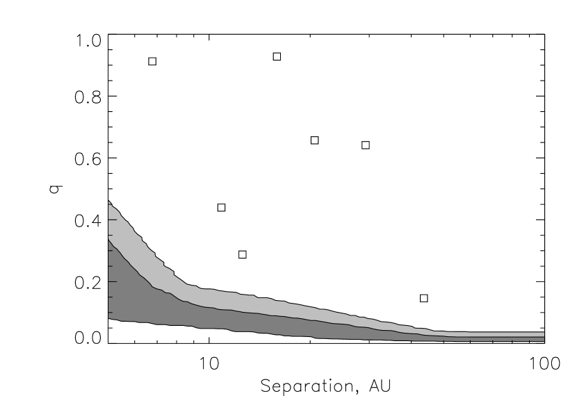
Figure 3: Mass ratios $q=M_{2}/M_{1}$ of 7 the resolved sub-systems versus their projected separations. The shaded region indicates incomplete detections (light grey corresponds to detection probabilities from 0.5 to 0.9, dark grey from 0.1 to 0.5).

$K$-band absolute magnitudes $M_{K}$ of all companions were computed based on the photometry from 2MASS (see Table 1) and trigonometric parallaxes $\pi_{\rm HIP}$ from Hipparcos. For resolved pairs, we assume that the $\Delta m$ in the red NICI channel correspond to magnitude differences in the $K$-band. The masses were estimated from $M_{K}$ using the empirical relations of Henry & McCarthy (1993). We also tried a quadratic approximation of relation between mass and $M_{K}$ from Girardi et al. (2000). The relative difference with Henry & McCarthy (1993) is less than 10% for masses above 0.1 $M_{\odot}$. We checked that the influence of using either of these relations on the final result is not critical. Table 3 lists the estimated masses of the companions in the resolved sub-systems, their projected separations $r=\rho/\pi_{\rm HIP}$ and order-of-magnitude period estimates $P^{*}=r^{3/2}(M_{1}+M_{1})^{-1/2}$.

Table 3: Estimated parameters of the 7 observed sub-systems in wide binaries

HIP	Comp	$M_{1}$	$M_{2}$	r	$P^{*}$
		$M_{\odot}$	$M_{\odot}$	AU	yr
24711	Aa,Ab	1.04	0.15	43.6	260
43947	Aa,Ab	0.64	0.59	15.9	60
43947	Ba,Bb	0.55	0.24	10.9	40
44804	Aa,Ab	0.95	0.61	29.3	130
45734	Aa,Ab	0.88	0.81	6.8	14
49520	Ba,Bb	0.92	0.26	12.6	40
64498	Aa,Ab	1.09	0.71	20.6	70

Figure 3 shows the mass ratios $q=M_{2}/M_{1}$ in the resolved inner sub-systems as a function of projected separation. The median parallax of observed targets is 19 mas, so the upper limit of the separation range, 100 AU, corresponds to $\rho\approx 1.9^{\prime\prime}$. Maximum separations of dynamically stable sub-systems should not exceed 100 AU in most cases because the projected separations of the wide binaries range from 150 to 1000 AU (Table 1). Indeed, all detected sub-systems have $r<44$ AU. The lower limit of 5 AU corresponds to $\rho\approx 0.1^{\prime\prime}$, well above the NICI resolution limit.

The detection limits in the red channel were converted into mass ratios and averaged over the 61 observed components, producing a smooth detection probability $p_{\rm det}(r,q)$. Contours of this function at 0.1, 0.5, and 0.9 levels are over-plotted in Fig. 3. We see that the chosen region of the $(r,q)$ parameter space is well covered with NICI.

4.4 Statistical analysis

The purpose of this study is to reach statistical conclusions about the frequency and the properties of sub-systems in solar-type wide binaries. Considering the small number of components, we keep this analysis at a basic level, and assume that the mass ratios in secondary sub-systems have a power-law distribution independent of separation:

$$f(q)=\epsilon(\beta+1)q^{\beta}.$$ (2)

This model has only two free parameters, the total companion frequency $\epsilon$ and the power-law index $\beta$. Neglecting incomplete detection, the companion count gives $\epsilon=7/61=0.12\pm 0.04$.

The distribution of the companion projected separations in the considered range from 5 to 100 AU matters only because the detection limits depend on $r$. We assume that $f(\log r)={\rm const}$.

The input data are the $(r,q)$ values for $K=7$ sub-systems, the total number of surveyed targets $N=61$, and the array of detection probabilities $p_{\rm det}(r,q)$. We find the estimates of parameters $(\epsilon,\beta)$ by the Maximum Likelihood (ML) method (see e.g. Tokovinin et al., 2006, Apendix B). The likelihood function ${\cal L}$ is a product of the probabilities to obtain observations for each component (non-detections for $N-K$ systems or detections of $K$ subsystems with mass ratios $q_{k}$).

The minimum of $S=-2\ln{\cal L}$ is sought. This function depends on the input data and the model parameters as

$$S=2Nf_{0}-2\sum_{k=1}^{K}\ln[f(q_{k})p_{\rm det}(r_{k},q_{k})].$$ (3)

The summation over $k$ is done for the 7 detected companions. The companion probability $f_{0}$ equals the product $f(r,q)p_{\rm det}(r,q)$ averaged over the considered part of the parameter space $(r,q)$. If the detection probability $p_{\rm det}$ equals one everywhere, the result is $f_{0}=\epsilon$, otherwise $f_{0}<\epsilon$.

Figure 4: Contours of the $S$-function in the $\epsilon,\beta$ space corresponding to the 68% and 90% confidence areas. The minimum is marked with a cross.

The contours of $S$ in the parameter space define confidence limits: $\Delta S=1$ corresponds to the 68% interval (“$1\sigma$”), $\Delta S=2.71$ to 90% and $\Delta S=4$ to 95%, in direct analogy with the Gaussian probability distribution. We verified the ML method on a simulated data set. The input parameters were recovered and the confidence intervals were as expected.

Table 4: Confidence intervals

Interval	$\epsilon$	$\beta$
Min. $S$	0.12	0.18
68%	0.08…0.17	$-$0.30…0.80
90%	0.06…0.21	$-$0.54…1.28

Minimization of (3) leads to $(\epsilon,\beta)=(0.12,0.18)$. If we ignore the detection limits and set $p_{\rm det}=1$, the result changes little: $(\epsilon,\beta)=(0.11,0.40)$. The companion fraction 0.12 is not different from its naive estimate. As to the power index $\beta$, the ML points to a uniform distribution in $q$ as being most likely, although the uncertainty is large. The confidence areas of the parameters are shown in Fig. 4. Considering that the contours are not very elongated, we can determine the 68% and 90% confidence intervals for each parameter by a simple cross-section through the minimum (Table 4). The data are marginally compatible with $\beta\sim-0.5$, in which case the fraction of sub-systems may exceed 0.2 (see the lower-right extension of the 90% contour in Fig. 4).

5 Discussion

5.1 Completeness of the existing catalog

The fact that, in a sample of only 33 systems, six of the seven observed companions are new, shows that current knowledge of multiplicity among nearby solar-type systems is very incomplete, and that near-IR AO imaging is a powerful technique for detecting new companions.

Figure 5: Histograms of the mass-ratios in inner systems of triple stars. Solid lines correspond to the 123 close pairs and dashed lines to the 61 wide pairs. The vertical bars show $\pm\sqrt{N}$ statistical errors for each bin of width 0.2. All points are slightly displaced horizontally for clarity.

We plot in Fig. 5 the mass-ratio distribution in the inner sub-systems of known triple stars. The data are extracted from the updated version of the Multiple-Star Catalog (MSC, Tokovinin, 1997), where component masses are estimated by a variety of methods. We selected 220 systems within 200 pc from the Sun with masses of primary components from 0.5 to 1.5 $M_{\odot}$. They were sub-divided by the separation in the inner sub-systems in two groups, 123 close (semi-major axis $<1$ AU) and 61 wide (between 5 and 100 AU). The remaining 36 pairs have even wider separations. The mass-ratio distributions in these two groups are markedly different, but our un-biased survey results in a flat mass-ratio distribution, within errors. Therefore, the difference seen in Fig. 5 is caused by observational selection. Given an approximately equal number of close and wide sub-systems with large mass ratios (two last bins in Fig. 5) and assuming that the mass-ratio distributions in these two groups are indeed similar, we expect that the number of close and wide sub-systems (with separations below 1 AU and between 5 and 100 AU, respectively) are similar, too. The completeness of the MSC for wide sub-systems is thus about 1/2.

5.2 Companion fraction

Is the presence of a wide binary companion influencing the frequency of inner sub-systems? To answer this question, we compare our results on triples with surveys of solar-type binaries. Unfortunately, binary-star statistics are usually derived regardless of higher-order multiplicity, so a cleaner comparison must await new study of a large unbiased sample.

The separation range from 5 to 100 AU explored here corresponds to orbital periods between 10 y and 1000 y. According to Duquennoy & Mayor (1991), about 20% of solar-type dwarfs have companions with such periods. In the actual, narrower range of projected separations from 6.8 AU to 44 AU, 12% of solar-type dwarfs have companions. Therefore, the frequency of sub-systems around components of wide binaries is similar to the frequency of binary companions to single stars in the same separation range.

The frequency of sub-systems with periods below 3 y in visual multiples has been determined by Tokovinin & Smekhov (2002) to be between 11% and 18%. Again, it turned out to equal within observational errors the companion frequency among single dwarfs of similar masses in the solar neighborhood and in some open clusters. Desidera et al. (2006) surveyed RVs of 56 wide visual pairs and found that $0.135\pm 0.05$ fraction of companions have spectroscopic sub-systems.

Therefore, one might surmise that the presence of a wide companion does not affect the formation of inner, closer sub-systems in a wide range of separations. This question is however far from having been settled for both stellar and planetary sub-systems (see the discussion in Eggenberger et al., 2007). We know that almost all close binaries with periods below 3 d do have additional outer companions, although the mass ratios of close binaries with and without tertiary companions have identical distributions (Tokovinin et al., 2006).

5.3 Is the mass-ratio distribution universal?

Metchev & Hillenbrandt (2009) advocate the idea of a companion mass function with a universal power law over a wide range of separations and masses. They fit the mass-ratio distribution in solar-mass visual binaries to a power law with $\beta=-0.39\pm 0.36$. Visual companions to stars more massive than the Sun follow a power law $f(q)\propto q^{\beta}$ with $\beta$ from $-0.3$ to $-0.5$, as established in AO imaging surveys by Shatsky & Tokovinin (2002) and Kouwenhoven et al. (2005). Certainly, these distributions do not correspond to the most simplistic case of random companion pairing, as described in detail by Kouwenhoven et al. (2009).

Our survey of triples points to a flat mass-ratio distribution with $\beta\sim 0$. The errors are large, so the difference with visual binaries is not yet significant. The mass-ratio distribution in closer, spectroscopic binaries is approximately flat (Mazeh et al., 2003; Halbwachs et al., 2003), similar to the mass-ratio distribution in close sub-systems of triple stars (Fig. 5). If we confirm on a larger sample that sub-systems in triples do differ from pure binaries in their mass-ratio distribution, its universality will be seriously challenged.

5.4 Brown-dwarf desert

The mass function of companions to binary and multiple stars is radically different from the Initial Mass Function. Therefore, the fraction of low-mass companions is much smaller than the fraction of low-mass stars in the field. This fact, known as brown dwarf (BD) desert, is well established (Grether & Lineweaver, 2006). Adopting a flat mass-ratio distribution for our sample, also typical for spectroscopic binaries, we estimate that only 7% of companions to a solar-mass star will be in the BD regime. Considering the companion frequency of 0.12 in the studied separation range, one BD companion per $\sim$100 primaries is expected. Our result thus suggests that the BD desert in multiple systems extends to separations of 100 AU.

The BD desert and the tendency to equal companion masses are explained in the current star-formation scenario by continuing accretion onto a binary. Whenever a low-mass companion forms by fragmentation of a massive disk, continuing accretion usually brings its mass into stellar regime (e.g. Kratter et al., 2010). Companions of sub-stellar masses should be intrinsically rare. At the same time the orbital drag (inward migration) reduces the separation, producing close sub-systems. It appears that about half of the companions settle in close orbits with separation $<1$ AU, the rest of them remain in wider orbits.

6 Conclusions

We surveyed 33 nearby wide binaries with solar-type primaries and found 7 resolved sub-systems, most of them previously unknown. We derive the fraction of sub-systems with projected separations from 5 to 100 AU to be $0.12\pm 0.04$. The mass-ratio distribution in these sub-systems appears to be flat, to within a large statistical error.

The sample can be increased 6 times if we continue observations with NICI and extend them to the Northern sky using some other AO facility. Such investment of 5 nights on 8-m telescopes will enable to reduce the size of the confidence intervals in Fig. 4 by 2.5 times. Then, it will become possible to distinguish between the negative power index $\beta\sim-0.3$ typical for resolved binaries and flat mass-ratio distribution $\beta\sim 0$ characteristic of close binaries.

The joint fraction of both visual and spectroscopic sub-systems in wide solar-type binaries is about 0.25. In consequence, the majority of the components are single, and provide an accomodating environment to host planetary systems.

References

- Artigau et al. (2008) Artigau, E., Biller, B. A., Wahhaj, Z., Hartung, M., Hayward, T. L., Close, L. M., Chun, M. R., Liu, M. C., Trancho, G., Rigaut, F. et al. 2008, in: Ground-based and Airborne Instrumentation for Astronomy II. Ed. McLean, I. S. & Casali, M. Proc. SPIE, 7014, 66
- Bate (2009) Bate, M. R. 2009, MNRAS, 392, 590
- Biller et al. (2008) Biller, B., Artigaut, É., Wahhaj, Z., Hartung, M., Liu, M.-C., Close, L. M., Chun, M. R., Ftaclas, C., Toomey, D. W., & Hayward, T. 2008, In: Proc. SPIE, 7015, 184
- Chauvin et al. (2010) Chauvin, G., Lagrange, A.-M., Bonavita, M., Zuckerman, B., Dumas, C., Bessell, M. S., Beuzit, J.-L., Bonnefoy, M., Desidera, S., Farihi, J., Lowrance, P., Mouillet, D., & Song, I. 2010, A&A, 509, A52
- Chun et al. (2008) Chun, M. Toomey, D., Wahhaj, Z., Biller, B., Artigau, E., Hayward, T., Liu, M., Close, L., Hartung, M., Rigaut, F., & Ftaclas, Ch. 2008, in: Adaptive Optics Systems. Ed. Hubin, N., Max, C. E., Wizinowich, P. L. Proc. SPIE, 7015, 70151V
- Covino et al. (1997) Covino, E., Alcala, J. M., Allain, S., et al. 1997, A&A, 328, 187
- Cutri et al. (2003) Cutri, R. M., Skrutskie, M. F., van Dyk, S., Beichman, C. A., Carpenter, J. M., Chester, T., Cambresy, L., Evans, T., Fowler, J., Gizis, J. et al. 2003, The IRSA 2MASS All-Sky Point Source Catalog. NASA/IPAC Infrared Science Archive.
- Desidera et al. (2006) Desidera, S., Gratton, R. G., Lucatello, S., Claudi, R. U., & Dall, T.H. 2006, A&A, 454, 553
- Duquennoy & Mayor (1991) Duquennoy, A. & Mayor, M. 1991, A&A 248, 485
- Eggenberger et al. (2007) Eggenberger, A., Udry, S., Chauvin, G., Beuzit, J.-L., Lagrange, A.-M., Ségransan, D., & Mayor, M. 2007, A&A, 474, 273
- ESA (1997) ESA 1997, The Hipparcos and Tycho Catalogues, ESA SP-1200
- Girardi et al. (2000) Girardi, L., Bressan, A., Bertelli, G., & Chiosi, C., 2000, A&AA, 141, 371
- Grether & Lineweaver (2006) Grether, D. & Lineweaver, C.H. 2006, ApJ, 640, 1051
- Halbwachs et al. (2003) Halbwachs, J. L., Mayor, M., Udry, S., & Arenou, F. 2003, A&A, 397, 159
- Harrington (1972) Harrington, R. S. 1972, Celest. Mech., 6, 322
- Henry & McCarthy (1993) Henry, T. J. & McCarthy, D. W. 1993, AJ, 106, 773
- Köhler (2001) Köhler, R. 2001, AJ, 122, 3325
- Kouwenhoven et al. (2005) Kouwenhoven, M. B. N., Brown, A. G. A., Zinnecker, H., Kaper, L., & Portegies Zwart, S. F. 2005, A&A, 430, 137
- Kouwenhoven et al. (2009) Kouwenhoven, M. B. N., Brown, A. G. A., Goodwin, S. P., Portegies Zwart, S. F., & Kaper, L. 2009, A&A, 493, 979
- Kratter et al. (2010) Kratter, K. M., Murray-Clay, R. A., & Youdin, A. N. 2010, ApJ, 710, 1375
- Mason et al. (2001) Mason, B. D., Wycoff, G. L., Hartkopf, W. I., Douglass, G. G. & Worley, C. E. 2001, AJ 122, 3466 (see the current version at http://www.usno.navy.mil/USNO/astrometry/optical-IR-prod/wds/wds.html)
- Mazeh et al. (2003) Mazeh, T., Simon, M., Prato, L., Markus, B., & Zucker, S. 2003, ApJ, 599, 1344