Simple models of bouncing ball dynamics and their comparison

Abstract

Nonlinear dynamics of a bouncing ball moving in gravitational field and colliding with a moving limiter is considered. Several simple models of table motion are studied and compared. Dependence of displacement of the table on time, approximating sinusoidal motion and making analytical computations possible, is assumed as quadratic and cubic functions of time, respectively.

1 Introduction

Vibro-impacting systems belong to a very interesting and important class of nonsmooth and nonlinear dynamical systems [1, 2, 3, 4] with important technological applications [5, 6, 7, 8]. Dynamics of such systems can be extremely complicated due to velocity discontinuity arising upon impacts. A very characteristic feature of such systems is the presence of nonstandard bifurcations such as border-collisions and grazing impacts which often lead to complex chaotic motions.

The Poincaré map, describing evolution from an impact to the next impact, is a natural tool to study vibro-impacting systems. The main difficulty with investigating impacting systems is in finding instant of the next impact what typically involves solving a nonlinear equation. However, the problem can be simplified in the case of a bouncing ball dynamics assuming a special motion of the limiter. Bouncing ball models have been extensively studied, see [9] and references therein. As a motivation that inspired this work, we mention study of physics and transport of granular matter [6]. A similar model has been also used to describe the motion of railway bogies [7].

Recently, we have considered several models of motion of a material point in a gravitational field colliding with a limiter moving with piecewise constant velocity [10, 11, 12, 13, 14]. In the present paper more realistic yet still simple models are considered. The purpose of this work is to approximate sinusoidal motion as exactly as possible but still preserving possibility of analytical computations.

The paper is organized as follows. In Section 2 a one dimensional dynamics of a ball moving in a gravitational field and colliding with a table is considered and Poincaré map is constructed. Dependence of displacement of the table on time is assumed as quadratic and cubic functions of time, respectively. In Section 3 bifurcation diagrams for such models of table motion are computed and compared with the case of sinusoidal motion.

2 Bouncing ball: a simple motion of the table

We consider a motion of a small ball moving vertically in a gravitational field and colliding with a moving table, representing unilateral constraints. The ball is treated as a material point while the limiter’s mass is assumed so large that its motion is not affected at impacts. A motion of the ball between impacts is described by the Newton’s law of motion:

$$m\ddot{x}=-mg,$$ (1)

where $\dot{x}=dx/dt$ and motion of the limiter is:

$$y=y\left(t\right),$$ (2)

with a known function $y$. We shall also assume that $y$ is a continuous function of time. Impacts are modeled as follows:

$$x\left(\tau_{i}\right) = y\left(\tau_{i}\right),$$ (3)

$$\dot{x}\left(\tau_{i}^{+}\right)-\dot{y}\left(\tau_{i}\right) = -R\left(\dot{x}\left(\tau_{i}^{-}\right)-\dot{y}\left(\tau_{i}\right)\right),$$ (4)

where duration of an impact is neglected with respect to time of motion between impacts. In Eqs. (3), (4) $\tau_{i}$ stands for time of the $i$-th impact while $\dot{x}_{i}^{-}$, $\dot{x}_{i}^{+}$are left-sided and right-sided limits of $\dot{x}_{i}\left(t\right)$ for $t\rightarrow\tau_{i}$, respectively, and $R$ is the coefficient of restitution, $0\leq R<1$ [5].

Solving Eq. (1) and applying impact conditions (3), (4) we derive the Poincaré map [15]:

$$\gamma Y\left(T_{i+1}\right) = \gamma Y\left(T_{i}\right)-\Delta_{i+1}^{2}+\Delta_{i+1}V_{i},$$ (5a)

$$V_{i+1} = -RV_{i}+2R\Delta_{i+1}+\gamma\left(1+R\right)\dot{Y}\left(T_{i+1}\right),$$ (5b)

where $$\Delta_{i+1}\equiv T_{i+1}-T_{i} Y_{s}(T)=\sin(T) T_{i+1}$$. The limiter’s motion has been typically assumed in form , cf. [11] and references therein. This choice leads to serious difficulties in solving the first of Eqs.(5) for , thus making analytical investigations of dynamics hardly possible. Accordingly, we have decided to simplify the limiter’s periodic motion to make (5a) solvable.

In our previous papers we have assumed displacement of the table as the following periodic function of time:

$$Y\left(T\right)=\left\{\begin{array}[]{l}\frac{1}{h}\hat{T},\quad 0\leq\hat{T}<h\\ \frac{-1}{1-h}\hat{T}+\frac{1}{1-h},\quad h\leq\hat{T}\leq 1\end{array}\right.$$ (6)

with $\hat{T}=T-\left\lfloor T\right\rfloor$ and $0<h<1$, where $\left\lfloor x\right\rfloor$ is the floor function – the largest integer less than or equal to $x$. In this work the function $Y(T)$ is assumed as quadratic $Y_{q}$ and two cubic functions of time, $Y_{c_{1}}$ and $Y_{c_{2}}$. More exactly, these functions read:

$$Y_{q}\left(T\right)=\left\{\begin{array}[]{l}-16\hat{T}\left(\hat{T}-\frac{1}{2}\right),\quad 0\leq\hat{T}<\frac{1}{2}\\ 16\left(\hat{T}-\frac{1}{2}\right)\left(\hat{T}-1\right),\quad\frac{1}{2}\leq\hat{T}\leq 1\end{array}\right.$$ (7)

$$Y_{c_{1}}\left(T\right)=12\sqrt{3}\hat{T}\left(\hat{T}-\frac{1}{2}\right)\left(\hat{T}-1\right),\quad 0\leq\hat{T}\leq 1$$ (8)

$$Y_{c_{2}}\left(T\right)=\left\{\begin{array}[]{cc}\left(32\pi-128\right)\hat{T}^{3}+\left(-16\pi+48\right)\hat{T}^{2}+2\pi\hat{T}&0\leq\hat{T}<\frac{1}{4}\\ \left(128-32\pi\right)\hat{T}^{3}+\left(-144+32\pi\right)\hat{T}^{2}+\left(48-10\pi\right)\hat{T}-4+\pi&\frac{1}{4}\leq\hat{T}<\frac{1}{2}\\ \left(128-32\pi\right)\hat{T}^{3}+\left(-240+64\pi\right)\hat{T}^{2}+\left(144-42\pi\right)\hat{T}-28+9\pi&\frac{1}{2}\leq\hat{T}<\frac{3}{4}\\ \left(32\pi-128\right)\hat{T}^{3}+\left(336-80\pi\right)\hat{T}^{2}+\left(-288+66\pi\right)\hat{T}+80-18\pi&\frac{3}{4}\leq\hat{T}\leq 1\end{array}\right.$$ (9)

see Figs. 1 ,2, 3.

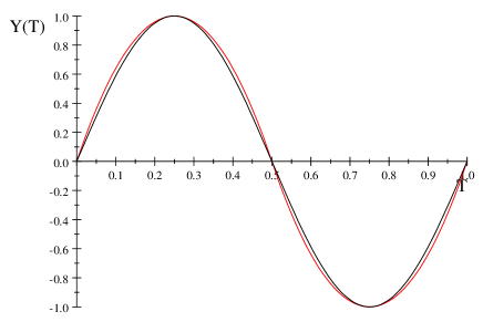
Figure 1: Displacement of the table, $Y_{q}(T)$ (black) and $Y_{s}(T)$ (red).

The function $Y_{q}$, consisting of two parabolas, and its first derivative are continuous, however its second derivative is discontinuous at $T=0,\ \frac{1}{2},\ 1$. The function $Y_{c_{1}}$ is smooth but provides a poorer approximation to $Y_{s}\left(T\right)=\sin\left(2\pi T\right)$ then $Y_{q}$. We have included this function because it is smooth and is the lowest-order polynomial approximating $Y_{s}$ on the unit interval $\left[0,\ 1\right]$.

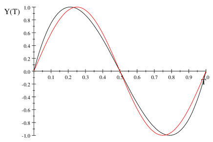
Figure 2: Displacement of the table, $Y_{c_{1}}(T)$ (black) and $Y_{s}(T)$ (red).

The smooth function $Y_{c_{2}}$ consists of four cubic functions and provides the best approximation to $Y_{s}$. Let us note that for all these functions, $Y_{q}$, $Y_{c_{1}}$, $Y_{c_{2}}$, equation for $T_{i+1}$, cf. Eq. (5a), is solvable.

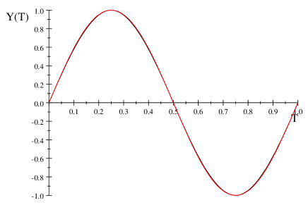
Figure 3: Displacement of the table, $Y_{c_{2}}(T)$ (black) and $Y_{s}(T)$ (red).

Our model consists thus of equation (5) and one of Eqs.(7), (8), (9) with control parameters $R$, $\gamma$. Since the period of motion of the limiter is equal to one, the map (5) is invariant under the translation $T_{i}\rightarrow T_{i}+1$. Accordingly, all impact times $T_{i}$ can be reduced to the unit interval $\left[0,\ 1\right]$.

3 Comparison of bifurcation diagrams

We have computed bifurcation diagrams to study dependence of dynamics on the model of motion of the table. Let us recall that in the case of displacement of the table described by piecewise linear function $Y$ defined in Eq.(6) the bifurcation diagram differs significantly from that computed for sinusoidal displacement $Y_{s}$.

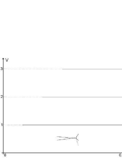
Figure 4: Bifurcation diagram, $Y(T)=Y_{q}(T)$

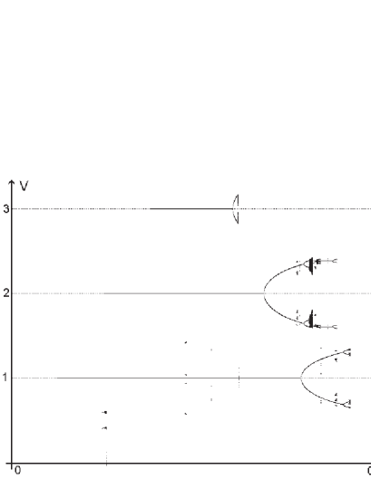
Figure 5: Bifurcation diagram, $Y(T)=Y_{c_{1}}(T)$

In the $h\rightarrow 1$ case only manifolds of periodic solutions were found to exist and there is no chaotic dynamics [11] while for $h\neq 1$, classical attractors exist as well, but only one period doubling on route to chaos via corner bifurcation was reported [13] in contradistinction to the case of sinusoidal displacement of the table where full period doubling scenario is generic [15].

The bifurcation diagram for the displacement function $Y_{q}$ is shown in Fig. 4. There are one 2-cycle (ending after one period doubling) and six fixed points (first three are shown) which become unstable at some $\gamma_{cr}$ where chaotic bands appear. There are no manifolds of periodic solutions. The bifurcation diagrams for functions $Y_{c_{1}}$ and $Y_{c_{2}}$ are presented in Figs. 5 and 6, respectively. It can be seen that full cascades of period doubling with transition to chaos are present in Fig. 5 but it seems that some bifurcation paths end abruptly. Moreover, periodic states loose stability in different order than for $Y_{s}$.

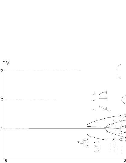
Figure 6: Bifurcation diagram, $Y(T)=Y_{c_{2}}(T)$

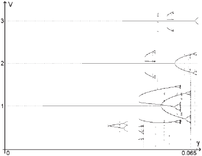
Figure 7: Bifurcation diagram, $Y(T)=sin\left(2\pi T\right)$

We note finally that the bifurcation diagram computed for the displacement function $Y_{c_{2}}$, cf. Fig. 6, is very similar to the bifurcation diagram for the sine function $Y_{s}$, see Fig. 7.

4 Summary and discussion

We have constructed several simple models of table motion in bouncing ball dynamics in order to approximate sinusoidal motion as exactly as possible. In conclusion we can state that dynamics of the model based on Eqs. (5), (9) corresponds well to dynamics with table displacement given by $Y_{s}\left(T\right)=\sin\left(2\pi T\right)$. Moreover, equation for time of the next impact (5a) is a third-order algebraic equation in $T_{i+1}$ for $Y\left(T\right)=Y_{c_{2}}\left(T\right)$ and thus analytical computations are possible. We are going to investigate all these models in our future work.

References

- [1] M. di Bernardo, C.J. Budd, A.R. Champneys, P. Kowalczyk, Piecewise-Smooth Dynamical Systems. Theory and Applications. Series: Applied Mathematical Sciences, vol. 163. Springer, Berlin (2008).
- [2] A.C.J.Luo, Singularity and Dynamics on Discontinuous Vector Fields. Monograph Series on Nonlinear Science and Complexity, vol. 3. Elsevier, Amsterdam (2006).
- [3] J. Awrejcewicz, C.-H. Lamarque, Bifurcation and Chaos in Nonsmooth Mechanical Systems.World Scientific Series on Nonlinear Science: Series A, vol. 45. World Scientific Publishing, Singapore (2003).
- [4] A.F. Filippov, Differential Equations with Discontinuous Right-Hand Sides. Kluwer Academic, Dordrecht (1988).
- [5] W.J. Stronge, Impact mechanics. Cambridge University Press, Cambridge (2000).
- [6] A. Mehta (ed.), Granular Matter: An Interdisciplinary Approach. Springer, Berlin (1994).
- [7] C. Knudsen, R. Feldberg, H. True, Bifurcations and chaos in a model of a rolling wheel-set. Philos. Trans. R. Soc. Lond. A 338 (1992) 455–469.
- [8] M. Wiercigroch, A.M. Krivtsov, J. Wojewoda, Vibrational energy transfer via modulated impacts for percussive drilling. Journal of Theoretical and Applied Mechanics 46 (2008) 715-726.
- [9] A. C. J. Luo, Y. Guo, Motion Switching and Chaos of a Particle in a Generalized Fermi-Acceleration Oscillator, Mathematical Problems in Engineering, vol. 2009, Article ID 298906, 40 pages, 2009. doi:10.1155/2009/298906.
- [10] A. Okninski, B. Radziszewski, Dynamics of impacts with a table moving with piecewise constant velocity, Vibrations in Physical Systems, vol. XXIII, p.289 – 294, C. Cempel, M.W. Dobry (Editors), Poznań 2008.
- [11] A. Okninski, B. Radziszewski, Dynamics of a material point colliding with a limiter moving with piecewise constant velocity, in: Modelling, Simulation and Control of Nonlinear Engineering Dynamical Systems. State-of-the Art, Perspectives and Applications, J. Awrejcewicz (Ed.), Springer 2009, pp. 117-127.
- [12] A. Okninski, B. Radziszewski, Dynamics of impacts with a table moving with piecewise constant velocity, Nonlinear Dynamics 58 (2009) 515-523.
- [13] A. Okninski, B. Radziszewski, Chaotic dynamics in a simple bouncing ball model, Proceedings of the 10th Conference on Dynamical Systems: Theory and Applications, December 7-10, 2009. Łódź, Poland, J. Awrejcewicz, M. Kazmierczak, P. Olejnik, J. Mrozowski (eds.), pp. 651-656.
- [14] Chaotic dynamics in a simple bouncing ball model, arXiv:1002.2448 [nlin.CD].
- [15] A. Okninski, B. Radziszewski, Grazing dynamics and dependence on initial conditions in certain systems with impacts, arXiv:0706.0257 (2007).