Nonperturbative Pauli–Villars regularization
of vacuum polarization in light-front QED

Abstract

We continue the development of a nonperturbative light-front Hamiltonian method for the solution of quantum field theories by considering the one-photon eigenstate of Lorentz-gauge QED. The photon state is computed nonperturbatively for a Fock basis with a bare photon state and electron-positron pair states. The calculation is regulated by the inclusion of Pauli–Villars (PV) fermions, with one flavor to make the integrals finite and a second flavor to guarantee a zero mass for the physical photon eigenstate. We compute in detail the constraints on the PV coupling strengths that this zero mass implies. As part of this analysis, we provide the complete Lorentz-gauge light-front QED Hamiltonian with two PV fermion flavors and two PV photon flavors, which will be useful for future work. The need for two PV photons was established previously; the need for two PV fermions is established here.

I Introduction

The nonperturbative solution of quantum field theories is a very difficult problem. For weakly coupled theories, this is usually avoided, and perturbation theory is applied. For strongly coupled theories, in particular quantum chromodynamics, the nonperturbative problem cannot be avoided for long. Various nonperturbative methods have been developed, including lattice theory Lattice ; TransLattice , Dyson–Schwinger equations DSE , and light-front Hamiltonian approaches DLCQreview ; Glazek ; Karmanov ; Vary ; TwoPhotonQED , and have met with some success. The light-front methods have the distinct advantage of providing wave functions as part of the solution. The wave functions appear as coefficients in a Fock-state expansion for the Hamiltonian eigenstate.

Here we continue development of a particular light-front Hamiltonian method bhm ; YukawaOneBoson ; OnePhotonQED ; ChiralLimit ; Thesis ; SecDep ; TwoPhotonQED based on Pauli–Villars (PV) regularization PauliVillars . Much of the recent development has been in QED OnePhotonQED ; ChiralLimit ; Thesis ; SecDep ; TwoPhotonQED , where results can be checked against perturbation theory, but which shares the gauge-theory nature of QCD. However, there is no expectation of being able to compete with perturbative QED for accuracy; any but the lowest-order Fock-space truncations require numerical techniques, where the accuracy is typically on the order of 1%. Thus, the method is not likely to compete with perturbation theory for any weakly coupled theory, but this is not a flaw in a method intended for strongly coupled theories.

The previous work considered eigenstates of a fermion dressed by one or more scalar or vector bosons. Eventually we wish to extend the dressed-fermion calculations to include one or more fermion-antifermion pairs. As a first step in this direction, we consider the vacuum-polarization correction to the one-photon state of light-front QED. The Fock basis is then simply the bare photon state and the electron-positron states, plus their PV counterparts. This will allow us to understand how such states can be included in the dressing of an additional fermion.

The PV regularization method relies upon the introduction of heavy PV fields to the Lagrangian. Some are assigned a negative norm, and the interaction terms are built from zero-norm combinations of the fundamental fields. The negative norms provide the cancellations needed to regulate perturbation theory, and we find that the nonperturbative eigenvalue problem is then also regulated. The use of zero-norm combinations in the interactions eliminates YukawaOneBoson the instantaneous fermion contributions DLCQreview from the light-front Hamiltonian, and, in the case of a gauge theory, allows the use of gauges other than light-cone gauge OnePhotonQED . We discuss these features in more detail in the next section.

To regulate the dressed-electron problem, we used one PV Fermi field and two PV photon fields ChiralLimit . One of each is sufficient to make the integral equations finite, but the second PV photon flavor is needed to maintain the chiral symmetry of the massless-electron limit. For the present calculation of a photon dressed by an electron-positron pair, the PV photon flavors are of no particular consequence, but we find that we need two PV fermion flavors. One flavor is again enough to have a finite result, and the second is needed to maintain a zero mass for the photon. A zero mass is not otherwise guaranteed, because the zero-norm fields in the interaction Lagrangian generate flavor-changing currents that break gauge invariance OnePhotonQED .

The addition of a second PV fermion flavor to the older calculations of the dressed-electron state does not create any new difficulty, because we can simply take the infinite-mass limit for this flavor and remove it from the calculation. However, a new calculation of the dressed-electron state that includes electron-positron pairs will require the second PV fermion flavor.

As higher and higher Fock sectors are included in a calculation, the number of PV flavors should not change, in general. An exception for QED would be any Fock basis that includes the possibility of light-by-light scattering. The breaking of gauge invariance by the flavor-changing currents should ruin the usual automatic cancellation of divergences for this process. Additional PV fields or an explicit counterterm will be required, but we do not consider this further here.

Although the number of PV flavors need not change, their coupling strengths do need to change as more Fock states are added TwoPhotonQED . The conditions of chiral symmetry for massless electrons and zero mass for photons, which complete the determination of these couplings, become complicated nonlinear equations for the coupling coefficients. These typically require iterative techniques for their solution TwoPhotonQED . At one loop, the conditions can be solved analytically.

The analysis is done in terms of light-cone quantization DLCQreview ; Dirac . The coordinates are $x^{\pm}=x^{0}\pm x^{3}$ and $\vec{x}_{\perp}=(x^{1},x^{2})$, with $x^{+}$ chosen as the light-cone time coordinate and the three-vector of space coordinates written as $\underline{x}=(x^{-},\vec{x}_{\perp})$. The momentum conjugate to $x^{-}$ is $p^{+}$; therefore, the light-cone three-momentum is $\underline{p}=(p^{+},\vec{p}_{\perp})$. Dot products are given by $\underline{p}\cdot\underline{x}=\frac{1}{2}p^{+}x^{-}-\vec{p}_{\perp}\cdot\vec{x}_{\perp}$. The light-cone energy is $p^{-}$, and evolution in light-cone time is determined by the light-cone Hamiltonian ${\cal P}^{-}$. The mass eigenvalue problem, in a frame where the total transverse momentum $\vec{P}_{\perp}$ is zero, is given by ${\cal P}^{-}|\underline{P}\rangle=\frac{M^{2}}{P^{+}}|\underline{P}\rangle$.

The primary objective is the solution of this eigenvalue problem in a Fock basis, with the eigenstate $|\underline{P}\rangle$ expanded in terms of the Fock states with wave functions as the coefficients. The eigenvalue problem becomes a coupled set of integral equations for the wave functions. Truncation of the basis makes the coupled system finite. At very low orders of truncation, the system can be solved analytically; in general, numerical techniques are required TwoPhotonQED .

The contents of the remainder of the paper are as follows. In Sec. II, we summarize the formulation of light-front QED in Lorentz gauge, extended to include two PV fermion flavors and two PV photon flavors. We then construct the photon eigenstate dressed by fluctuations to an electron-positron pair in Sec. III and solve the eigenvalue problem to determine the coupling coefficients. Section IV contains a discussion of the results. An appendix describes the evaluation of a key integral.

II Light-front QED in Lorentz gauge

The Lorentz-gauge QED Lagrangian, regulated by two PV fermion flavors and two PV photon flavors, is

$${\cal L} = \sum_{i=0}^{2}(-1)^{i}\left[-\frac{1}{4}F_{i}^{\mu\nu}F_{i,\mu\nu}+\frac{1}{2}\mu_{i}^{2}A_{i}^{\mu}A_{i\mu}-\frac{1}{2}\left(\partial^{\mu}A_{i\mu}\right)^{2}\right]$$

$$+\sum_{i=0}^{2}(-1)^{i}\bar{\psi_{i}}(i\gamma^{\mu}\partial_{\mu}-m_{i})\psi_{i}-e_{0}\bar{\psi}\gamma^{\mu}\psi A_{\mu},$$

where

$$\psi=\sum_{i=0}^{2}\sqrt{\beta_{i}}\psi_{i},\;\;A_{\mu}=\sum_{i=0}^{2}\sqrt{\xi_{i}}A_{i\mu},\;\;F_{i\mu\nu}=\partial_{\mu}A_{i\nu}-\partial_{\nu}A_{i\mu}.$$ (2)

A subscript of $i=0$ indicates a physical field, and $i=1$ or 2 a PV field. The $i=1$ fields are chosen to have negative norm. The mass of the bare photon $\mu_{0}$ is zero; the mass of the bare electron $m_{0}$ is typically close to the physical electron mass $m_{e}$ for the range of PV masses usually considered TwoPhotonQED .

The constants $\beta_{i}$ and $\xi_{i}$ control the coupling strengths of the various fields. These coupling coefficients must satisfy constraints for the theory to be consistent. For $e_{0}$ to be the bare charge of the bare electron, we require $\beta_{0}=1$ and $\xi_{0}=1$. The cancellations necessary to regulate perturbation theory, which must arise in a sum over flavors of each internal line, require that $\sum_{i}(-1)^{i}\beta_{i}e_{0}^{2}$ be zero for a fermion line and $\sum_{i}(-1)^{i}\xi_{i}e_{0}^{2}$ zero for a photon line. We therefore require

$$\sum_{i=0}^{2}(-1)^{i}\beta_{i}=0,\;\;\sum_{i=0}^{2}(-1)^{i}\xi_{i}=0.$$ (3)

These also guarantee that the combinations $\psi$ and $A_{\mu}$ in (2) have zero norm. A third pair of constraints comes from requiring that the photon eigenstate have zero mass and that the mass of the electron eigenstate becomes zero when $m_{0}$ is set to zero. Since the first two pairs of constraints imply $\beta_{1}=1+\beta_{2}$ and $\xi_{1}=1+\xi_{2}$, this third pair completes the determination of the coefficients by providing implicit equations for $\beta_{2}$ and $\xi_{2}$. In Sec. III, we seek $\beta_{2}$; for discussion of $\xi_{2}$, see TwoPhotonQED .

The fermion fields $\psi_{i}$ are decomposed into dynamical and nondynamical parts $\psi_{i\pm}\equiv\Lambda_{\pm}\psi_{i}$ by the complementary projections $\Lambda_{\pm}\equiv\gamma^{0}\gamma^{\pm}/2$ DLCQreview ; LepageBrodsky . The nondynamical parts satisfy the following constraints ($i=0$,1,2), obtained from projecting the Dirac equation with $\Lambda_{-}$:

$$i(-1)^{i}\partial_{-}\psi_{i-}+e_{0}A_{-}\sqrt{\beta_{i}}\psi_{-} = (i\gamma^{0}\vec{\gamma}^{\perp})\cdot\left[(-1)^{i}\vec{\partial}_{\perp}\psi_{i+}-ie_{0}\sqrt{\beta_{i}}\vec{A}_{\perp}\psi_{+}\right]$$ (4)

$$-(-1)^{i}m_{i}\gamma^{0}\psi_{i+}.$$

Ordinarily, light-cone gauge ($A_{-}=A^{+}=0$) would be chosen, so that the constraint for $\psi_{i-}$ can be solved explicitly. However, for the construction of the light-front Hamiltonian, we are interested in only the combination $\psi_{-}=\sum_{i}\sqrt{\beta_{i}}\psi_{i-}$. The constraint for $\psi_{-}$ can be obtained from (4) by first multiplying with $(-1)^{i}\sqrt{\beta_{i}}$ and then summing over $i$, which yields

$$i\partial_{-}\psi_{-}=(i\gamma^{0}\vec{\gamma}^{\perp})\cdot\vec{\partial}_{\perp}\psi_{+}-\gamma^{0}\sum_{i}m_{i}\sqrt{\beta_{i}}\psi_{i+}.$$ (5)

The terms containing the photon field cancel because $\sum_{i}(-1)^{i}\beta_{i}=0$. The nondynamical field $\psi_{-}$ can then be constructed from a sum of $\psi_{i-}$ that satisfy the free-fermion constraint.

The mode expansion for the full Fermi field of the $i$th flavor can be written as

$$\psi_{i}=\frac{1}{\sqrt{16\pi^{3}}}\sum_{s}\int\frac{d\underline{k}}{\sqrt{k^{+}}}\left[b_{is}(\underline{k})e^{-i\underline{k}\cdot\underline{x}}u_{is}(\underline{k})+d_{i,-s}^{\dagger}(\underline{k})e^{i\underline{k}\cdot\underline{x}}v_{is}(\underline{k})\right].$$ (6)

The spinors are LepageBrodsky

$$u_{is}(\underline{k}) = \frac{1}{\sqrt{k^{+}}}(k^{+}+\vec{\alpha}_{\perp}\cdot\vec{k}_{\perp}+\beta m_{i})\chi_{s},$$ (7)

$$v_{is}(\underline{k}) = \frac{1}{\sqrt{k^{+}}}(k^{+}+\vec{\alpha}_{\perp}\cdot\vec{k}_{\perp}-\beta m_{i})\chi_{-s},$$ (8)

with

$$\chi_{+}=\frac{1}{\sqrt{2}}\left(\begin{array}[]{c}1\\ 0\\ 1\\ 0\end{array}\right),\;\;\chi_{-}=\frac{1}{\sqrt{2}}\left(\begin{array}[]{c}0\\ 1\\ 0\\ -1\end{array}\right),$$ (9)

and the nonzero anticommutators are

$$\{b_{is}(\underline{k}),b_{i^{\prime}s^{\prime}}^{\dagger}(\underline{k}^{\prime})\} = (-1)^{i}\delta_{ii^{\prime}}\delta_{ss^{\prime}}\delta(\underline{k}-\underline{k}^{\prime}),$$ (10)

$$\{d_{is}(\underline{k}),d_{i^{\prime}s^{\prime}}^{\dagger}(\underline{k}^{\prime})\} = (-1)^{i}\delta_{ii^{\prime}}\delta_{ss^{\prime}}\delta(\underline{k}-\underline{k}^{\prime}).$$

The mode expansion for the $i$th photon flavor is

$$A_{i\mu}=\frac{1}{\sqrt{16\pi^{3}}}\int\frac{d\underline{k}}{\sqrt{k^{+}}}\left[a_{i\mu}(\underline{k})e^{-i\underline{k}\cdot\underline{x}}+a_{i\mu}^{\dagger}(\underline{k})e^{i\underline{k}\cdot\underline{x}}\right],$$ (11)

with the commutator

$${[}a_{i\mu}(\underline{k}),a_{i^{\prime}\nu}^{\dagger}(\underline{k}^{\prime})]=(-1)^{i}\delta_{ii^{\prime}}\epsilon^{\mu}\delta_{\mu\nu}\delta(\underline{k}-\underline{k}^{\prime}).$$ (12)

The metric signature $\epsilon^{\mu}=(-1,1,1,1)$ is chosen for Gupta–Bleuler quantization GuptaBleuler ; GaugeCondition . Because we do not use light-cone gauge, there is no constraint on $A_{+}=A^{-}$, and, consequently, there will be no instantaneous photon interaction term DLCQreview in the Hamiltonian. The gauge condition $\partial^{\mu}A_{i\mu}=0$ is implemented as a projection on the Fock states GuptaBleuler ; GaugeCondition , as discussed in ChiralLimit and the next section.

We can now construct the light-front Hamiltonian ${\cal P}^{-}$. The interaction terms are determined by the spinor matrix elements

$$\bar{u}_{is^{\prime}}(p)\gamma^{+}u_{js}(q) = 2\sqrt{p^{+}q^{+}}\delta_{s^{\prime}s},$$ (13)

$$\bar{u}_{is^{\prime}}(p)\gamma^{-}u_{js}(q) = \left\{\begin{array}[]{ll}\frac{2}{\sqrt{p^{+}q^{+}}}[\vec{p}_{\perp}\cdot\vec{q}_{\perp}\pm i\vec{p}_{\perp}\times\vec{q}_{\perp}+m_{i}m_{j}],&s^{\prime}=s=\pm,\\ \mp\frac{2}{\sqrt{p^{+}q^{+}}}[m_{j}(p^{1}\pm ip^{2})-m_{i}(q^{1}\pm iq^{2})],&s^{\prime}=-s=\mp,\end{array}\right.$$ (16)

$$\bar{u}_{is^{\prime}}(p)\gamma_{\perp}^{l}u_{js}(q) = \left\{\begin{array}[]{ll}\frac{1}{\sqrt{p^{+}q^{+}}}[p^{+}(q^{l}\pm i\epsilon^{lk3}q^{k})+q^{+}(p^{l}\mp i\epsilon^{lk3}p^{k})],&s^{\prime}=s=\pm,\\ \mp\frac{1}{\sqrt{p^{+}q^{+}}}(m_{i}q^{+}-m_{j}p^{+})(\delta^{l1}\pm i\delta^{l2}),&s^{\prime}=-s=\mp,\end{array}\right.$$ (19)

$$\bar{u}_{is^{\prime}}(\underline{p})\gamma^{\mu}v_{js}(\underline{q}) = \left(\bar{v}_{js}(\underline{q})\gamma^{\mu}u_{is^{\prime}}(\underline{p})\right)^{*}=\left.\bar{u}_{is^{\prime}}(\underline{p})\gamma^{\mu}u_{js}(\underline{q})\right|_{m_{j}\rightarrow-m_{j}}^{s\rightarrow-s},$$ (20)

$$\bar{v}_{is^{\prime}}(\underline{p})\gamma^{\mu}v_{js}(\underline{q}) = \left.\bar{u}_{is^{\prime}}(\underline{p})\gamma^{\mu}u_{js}(\underline{q})\right|_{m_{j}\rightarrow-m_{j},\,m_{i}\rightarrow-m_{i}}^{s\rightarrow-s,\,s^{\prime}\rightarrow-s^{\prime}}.$$ (21)

These generalize matrix elements given in LepageBrodsky to the case of unequal masses, to accommodate the flavor-changing currents. The Hamiltonian is then found to be

$${\cal P}^{-} = \sum_{i,s}\int d\underline{p}\frac{m_{i}^{2}+p_{\perp}^{2}}{p^{+}}(-1)^{i}b_{i,s}^{\dagger}(\underline{p})b_{i,s}(\underline{p})$$

$$+\sum_{i,s}\int d\underline{p}\frac{m_{i}^{2}+p_{\perp}^{2}}{p^{+}}(-1)^{i}d_{i,s}^{\dagger}(\underline{p})d_{i,s}(\underline{p})$$

$$+\sum_{l,\mu}\int d\underline{k}\frac{\mu_{l}^{2}+k_{\perp}^{2}}{k^{+}}(-1)^{l}\epsilon^{\mu}a_{l\mu}^{\dagger}(\underline{k})a_{l\mu}(\underline{k})$$

$$+\sum_{i,j,l,s,\mu}\sqrt{\beta_{i}\beta_{j}\xi_{l}}\int d\underline{p}d\underline{q}\left\{b_{i,s}^{\dagger}(\underline{p})\left[b_{j,s}(\underline{q})V^{\mu}_{ij,2s}(\underline{p},\underline{q})\right.\right.$$

$$\left.\left.\rule{126.47249pt}{0.0pt}+b_{j,-s}(\underline{q})U^{\mu}_{ij,-2s}(\underline{p},\underline{q})\right]a_{l\mu}^{\dagger}(\underline{q}-\underline{p})\right.$$

$$+b_{i,s}^{\dagger}(\underline{p})\left[d_{j,s}^{\dagger}(\underline{q})\bar{V}^{\mu}_{ij,2s}(\underline{p},\underline{q})+d_{j,-s}^{\dagger}(\underline{q})\bar{U}^{\mu}_{ij,-2s}(\underline{p},\underline{q})\right]a_{l\mu}(\underline{q}+\underline{p})$$

$$-\left.d_{i,s}^{\dagger}(\underline{p})\left[d_{j,s}(\underline{q})\tilde{V}^{\mu}_{ij,2s}(\underline{p},\underline{q})+d_{j,-s}(\underline{q})\tilde{U}^{\mu}_{ij,-2s}(\underline{p},\underline{q})\right]a_{l\mu}^{\dagger}(\underline{q}-\underline{p})+H.c.\right\}\,,$$

The vertex functions $V$ and $U$ are as given in OnePhotonQED :

$$V^{0}_{ij\pm}(\underline{p},\underline{q}) = \frac{e_{0}}{\sqrt{16\pi^{3}}}\frac{\vec{p}_{\perp}\cdot\vec{q}_{\perp}\pm i\vec{p}_{\perp}\times\vec{q}_{\perp}+m_{i}m_{j}+p^{+}q^{+}}{p^{+}q^{+}\sqrt{q^{+}-p^{+}}},$$ (23)

$$V^{3}_{ij\pm}(\underline{p},\underline{q}) = \frac{-e_{0}}{\sqrt{16\pi^{3}}}\frac{\vec{p}_{\perp}\cdot\vec{q}_{\perp}\pm i\vec{p}_{\perp}\times\vec{q}_{\perp}+m_{i}m_{j}-p^{+}q^{+}}{p^{+}q^{+}\sqrt{q^{+}-p^{+}}},$$

$$V^{1}_{ij\pm}(\underline{p},\underline{q}) = \frac{e_{0}}{\sqrt{16\pi^{3}}}\frac{p^{+}(q^{1}\pm iq^{2})+q^{+}(p^{1}\mp ip^{2})}{p^{+}q^{+}\sqrt{q^{+}-p^{+}}},$$

$$V^{2}_{ij\pm}(\underline{p},\underline{q}) = \frac{e_{0}}{\sqrt{16\pi^{3}}}\frac{p^{+}(q^{2}\mp iq^{1})+q^{+}(p^{2}\pm ip^{1})}{p^{+}q^{+}\sqrt{q^{+}-p^{+}}},$$

$$U^{0}_{ij\pm}(\underline{p},\underline{q}) = \frac{\mp e_{0}}{\sqrt{16\pi^{3}}}\frac{m_{j}(p^{1}\pm ip^{2})-m_{i}(q^{1}\pm iq^{2})}{p^{+}q^{+}\sqrt{q^{+}-p^{+}}},$$

$$U^{3}_{ij\pm}(\underline{p},\underline{q}) = \frac{\pm e_{0}}{\sqrt{16\pi^{3}}}\frac{m_{j}(p^{1}\pm ip^{2})-m_{i}(q^{1}\pm iq^{2})}{p^{+}q^{+}\sqrt{q^{+}-p^{+}}},$$

$$U^{1}_{ij\pm}(\underline{p},\underline{q}) = \frac{\pm e_{0}}{\sqrt{16\pi^{3}}}\frac{m_{i}q^{+}-m_{j}p^{+}}{p^{+}q^{+}\sqrt{q^{+}-p^{+}}},$$

$$U^{2}_{ij\pm}(\underline{p},\underline{q}) = \frac{ie_{0}}{\sqrt{16\pi^{3}}}\frac{m_{i}q^{+}-m_{j}p^{+}}{p^{+}q^{+}\sqrt{q^{+}-p^{+}}}.$$

The other four vertex functions are related to these by

$$\bar{V}_{ij,2s}^{\mu}(\underline{p},\underline{q}) = \sqrt{\frac{q^{+}-p^{+}}{q^{+}+p^{+}}}\left.V_{ij,2s}^{\mu}(\underline{p},\underline{q})\right|_{m_{j}\rightarrow-m_{j}},$$ (24)

$$\bar{U}_{ij,2s}^{\mu}(\underline{p},\underline{q}) = \sqrt{\frac{q^{+}-p^{+}}{q^{+}+p^{+}}}\left.U_{ij,2s}^{\mu}(\underline{p},\underline{q})\right|_{m_{j}\rightarrow-m_{j}},$$

$$\tilde{V}_{ij,2s}^{\mu}(\underline{p},\underline{q}) = \sqrt{\frac{p^{+}-q^{+}}{q^{+}-p^{+}}}\left.V_{ij,2s}^{\mu}(\underline{q},\underline{p})\right|_{m_{j}\rightarrow-m_{j},\,m_{i}\rightarrow-m_{i}},$$ (25)

$$\tilde{U}_{ij,2s}^{\mu}(\underline{p},\underline{q}) = \sqrt{\frac{p^{+}-q^{+}}{q^{+}-p^{+}}}\left.U_{ij,2s}^{\mu}(\underline{q},\underline{p})\right|_{m_{j}\rightarrow-m_{j},\,m_{i}\rightarrow-m_{i}}.$$

The Hamiltonian does not contain any instantaneous fermion terms DLCQreview . They cancel between physical and PV contributions because they are independent of the fermion mass and proportional to $(-1)^{i}\beta_{i}$ for the $i$th flavor. The sum over flavors then yields $\sum_{i}(-1)^{i}\beta_{i}=0$. This is independent of the gauge choice and does not even require a gauge theory; the same cancellation happens in Yukawa theory YukawaOneBoson . The absence of instantaneous fermion and instantaneous photon contributions is important for numerical calculations, where such four-point interactions can greatly increase the computational load and matrix storage requirements; this is partial compensation for the increase in basis size brought by the PV fields.

III Dressed photon eigenstate

We construct the Fock-state expansion for the photon eigenstate of the light-front Hamiltonian. This requires some discussion of the projection that implements the gauge condition GaugeCondition ; ChiralLimit . From the eigenvalue problem we obtain coupled equations for the Fock-state wave functions. We are interested in the leading vacuum-polarization contribution and, therefore, truncate the Fock basis to include only the bare photon state and single-fermion-pair states. The requirement that the physical photon eigenstate have zero mass then completes the determination of the fermion coupling coefficients $\beta_{i}$.

III.1 Gauge Projection

The gauge condition $\partial^{\mu}A_{i\mu}=0$ is implemented as a projection that eliminates one linear combination of unphysical polarizations and leaves only a zero-norm contribution from unphysical polarizations that provides for the residual gauge freedom GaugeCondition ; ChiralLimit . Let $e_{\mu}^{(\lambda)}(\underline{k})$ be the polarization vectors, with $\underline{k}$ the photon three-momentum and $\lambda=0$,1,2,3. They satisfy the orthogonality properties

$$e^{(\lambda)\mu}e_{\mu}^{(\lambda^{\prime})}=-\epsilon^{\lambda}\delta_{\lambda\lambda^{\prime}}=g_{\lambda\lambda^{\prime}}$$ (26)

and, for the physical polarizations $\lambda=1$ and 2,

$$k^{\mu}e_{\mu}^{(\lambda)}=0\;\;\mbox{and}\;\;n^{\mu}e_{\mu}^{(\lambda)}=0,$$ (27)

with $n$ a timelike four-vector that reduces to $(1,0,0,0)$ in the frame where $\vec{k}_{\perp}=0$. The annihilation operator for a particular polarization is given by

$$a_{i}^{(\lambda)}(\underline{k})=-\epsilon^{\lambda}e^{(\lambda)\mu}(\underline{k})a_{i\mu}(\underline{k})$$ (28)

and satisfies the commutation relation

$$[a_{i}^{(\lambda)}(\underline{k}),a_{j}^{(\lambda^{\prime})\dagger}(\underline{k}^{\prime})]=(-1)^{i}\delta_{ij}\epsilon^{\lambda}\delta_{\lambda\lambda^{\prime}}\delta(\underline{k}-\underline{k}^{\prime}).$$ (29)

Because the positive-frequency part of the gauge condition is proportional to $k^{\mu}a_{i\mu}=(k\cdot n)(a_{i}^{(0)}-a_{i}^{(3)})$, the condition can be implemented by the projection $(a_{i}^{(0)}-a_{i}^{(3)})|\psi\rangle=0$ for all Fock states $|\psi\rangle$. This projection can be satisfied by building Fock states with the physical-polarization operators $a_{i}^{(1)\dagger}$ and $a_{i}^{(2)\dagger}$ and the zero-norm combination $(a_{i}^{(0)}-a_{i}^{(3)})/\sqrt{2}$. The zero norm guarantees that the projection condition is satisfied. It also means that the unphysical polarizations make no contribution to observables; they instead represent the residual gauge freedom of the Lorentz gauge. For the present purpose, we do not need to include the unphysical polarizations at all.

III.2 Eigenvalue Problem

With the truncation to at most one electron-positron pair, the Fock-state expansion for a photon eigenstate with polarization $\lambda=1$ or 2 and total three-momentum $\underline{P}$ is

$$|\psi^{(\lambda)}(\underline{P})\rangle=\sum_{l}z_{l}^{\lambda}a_{l}^{(\lambda)\dagger}(\underline{P})|0\rangle+\sum_{ijss^{\prime}}\int d\underline{k}C_{ijss^{\prime}}^{\lambda}(\underline{k})b_{is}^{\dagger}(\underline{k})d_{js^{\prime}}^{\dagger}(\underline{P}-\underline{k})|0\rangle.$$ (30)

Here $z_{l}^{\lambda}$ is the bare photon amplitude for the $l$th flavor, and $C_{ijss^{\prime}}^{\lambda}(\underline{k})$ is the two-body wave function for an electron of flavor $i$, spin $s$, and momentum $\underline{k}$, and a positron of favor $j$, spin $s^{\prime}$, and momentum $\underline{P}-\underline{k}$. We will work in a frame where the total transverse momentum $\vec{P}_{\perp}$ is zero.

This dressed photon state is to be an eigenstate of the light-front Hamiltonian ${\cal P}^{-}$ with eigenvalue $M_{\lambda}^{2}/P^{+}$. Of course, for the physical photon, $M_{\lambda}$ should be zero. In terms of the wave functions, the eigenvalue problem becomes the following coupled set of equations:

$$\frac{M_{\lambda}^{2}}{P^{+}}z_{l}^{\lambda}=\frac{\mu_{l}^{2}}{P^{+}}z_{l}^{\lambda}$$

$$+\sum_{ijss^{\prime}\mu}\int d\underline{k}(-1)^{i+j}\sqrt{\beta_{i}\beta_{j}\xi_{l}}C_{ijss^{\prime}}^{\lambda}(\underline{k})e_{\mu}^{(\lambda)}(\underline{P})[\delta_{s^{\prime}s}\bar{V}_{ij,2s}^{\mu*}(\underline{k},\underline{P}-\underline{k})+\delta_{s^{\prime},-s}\bar{U}_{ij,-2s}^{\mu*}(\underline{k},\underline{P}-\underline{k})],$$

$$\frac{M_{\lambda}^{2}}{P^{+}}C_{ijss^{\prime}}^{\lambda}(\underline{k})=\left(\frac{m_{i}^{2}+k_{\perp}^{2}}{k^{+}}+\frac{m_{j}^{2}+k_{\perp}^{2}}{P^{+}-k^{+}}\right)C_{ijss^{\prime}}^{\lambda}(\underline{k})$$

$$+\sum_{k\mu}z_{k}^{\lambda}(-1)^{k}\sqrt{\beta_{i}\beta_{j}\xi_{k}}\epsilon^{\lambda}e_{\mu}^{(\lambda)}(\underline{P})[\delta_{s^{\prime}s}\bar{V}_{ij,2s}^{\mu}(\underline{k},\underline{P}-\underline{k})+\delta_{s^{\prime},-s}\bar{U}_{ij,-2s}^{\mu}(\underline{k},\underline{P}-\underline{k})].$$

We can then solve explicitly for the two-body wave function, written here in terms of $x\equiv k^{+}/P^{+}$,

$$C_{ijss^{\prime}}^{\lambda}(\underline{k})=\epsilon^{\lambda}\left(\sum_{k}(-1)^{k}\sqrt{\beta_{i}\beta_{j}\xi_{k}}\right)\sum_{\mu}\frac{P^{+}e_{\mu}^{(\lambda)}[\delta_{s^{\prime}s}\bar{V}_{ij,2s}^{\mu}(\underline{k},\underline{P}-\underline{k})+\delta_{s^{\prime},-s}\bar{U}_{ij,-2s}^{\mu}(\underline{k},\underline{P}-\underline{k})]}{M_{\lambda}^{2}-\frac{m_{i}^{2}+k_{\perp}^{2}}{x}-\frac{m_{j}^{2}+k_{\perp}^{2}}{1-x}}.$$ (33)

Substitution into the first equation, (III.2), and use of the vertex functions (24), yields

$$M_{\lambda}^{2}z_{l}^{\lambda}=\mu_{l}^{2}z_{l}^{\lambda}+m_{e}^{2}\sqrt{\xi_{l}}\epsilon^{\lambda}I(M_{\lambda}^{2})\sum_{k}(-1)^{k}\sqrt{\xi_{k}}z_{k}^{\lambda},$$ (34)

with $m_{e}$ the physical mass of the electron and

$$I(M^{2})=\frac{e_{0}^{2}}{8\pi^{3}}\sum_{ij}(-1)^{i+j}\frac{\beta_{i}\beta_{j}}{m_{e}^{2}}\int\frac{dxd^{2}k_{\perp}}{x(1-x)}\frac{(1-2x)^{2}k_{1}^{2}+k_{2}^{2}+(m_{i}(1-x)+m_{j}x)^{2}}{\left[M^{2}x(1-x)-(m_{i}^{2}+k_{\perp}^{2})(1-x)-(m_{j}^{2}+k_{\perp}^{2})x\right]}.$$ (35)

The form given for $I$ is explicitly for the $\lambda=1$ case; however, for $\lambda=2$, the first two terms in the numerator are replaced by $k_{1}^{2}+(1-2x)^{2}k_{2}^{2}$, which is actually equivalent due to the symmetry of the rest of the integrand with respect to the interchange of $k_{1}$ and $k_{2}$. Therefore, $I$ need not carry a polarization label, and the eigenmasses $M_{1}$ and $M_{2}$ are equal, as one would expect. Also, the cancellations provided by the PV fermions are sufficient to render $I(M^{2})$ finite.

III.3 Analytic Solution

The remaining equation, (34), is a $3\times 3$ matrix eigenvalue problem

$$H\vec{z}^{\lambda}=\frac{M^{2}}{m_{e}^{2}}\vec{z}^{\lambda},$$ (36)

where $\vec{z}^{\lambda}=(z_{0}^{\lambda},z_{1}^{\lambda},z_{2}^{\lambda})^{T}$ and

$$H=\left(\begin{array}[]{ccc}\mu_{0}^{2}/m_{e}^{2}+\xi_{0}I(M^{2})&-\sqrt{\xi_{0}\xi_{1}}I(M^{2})&\sqrt{\xi_{0}\xi_{2}}I(M^{2})\\ \sqrt{\xi_{0}\xi_{1}}I(M^{2})&\mu_{1}^{2}/m_{e}^{2}-\xi_{1}I(M^{2})&\sqrt{\xi_{1}\xi_{2}}I(M^{2})\\ \sqrt{\xi_{0}\xi_{2}}I(M^{2})&-\sqrt{\xi_{1}\xi_{2}}I(M^{2})&\mu_{2}^{2}/m_{e}^{2}+\xi_{2}I(M^{2})\end{array}\right).$$ (37)

When the bare photon mass $\mu_{0}$ is zero, the determinant of $H$ is

$${\rm det}H=\xi_{0}\frac{\mu_{1}^{2}\mu_{2}^{2}}{m_{e}^{4}}I(M^{2}).$$ (38)

Therefore, the physical photon eigenstate has zero mass, within the given truncated Fock basis, if and only if $I(0)$ is zero. This provides the condition for determination of the coupling coefficient $\beta_{2}$.

The integrals in $I(0)$ are simple enough to permit its analytic evaluation. This is presented in the Appendix, with the result that

$$I(0)=\frac{e_{0}^{2}}{8\pi^{2}}\sum_{ij}(-1)^{i+j}\beta_{i}\beta_{j}I_{ij},$$ (39)

with the $I_{ij}$ given in (46).

To use $I(0)=0$ to find $\beta_{2}$, we replace $\beta_{0}=1$ and $\beta_{1}=1+\beta_{2}$, and take advantage of the symmetry $I_{ij}=I_{ji}$, to write $I(0)=0$ as

$$I_{00}+I_{11}-2I_{01}+2(I_{11}+I_{02}-I_{01}-I_{12})\beta_{2}+(I_{11}+I_{22}-2I_{12})\beta_{2}^{2}=0.$$ (40)

The two roots of this quadratic equation are plotted in Fig. 1 as functions of the PV masses $m_{1}$ and $m_{2}$, with the bare electron mass set to a typical value for the dressed-electron problem TwoPhotonQED .

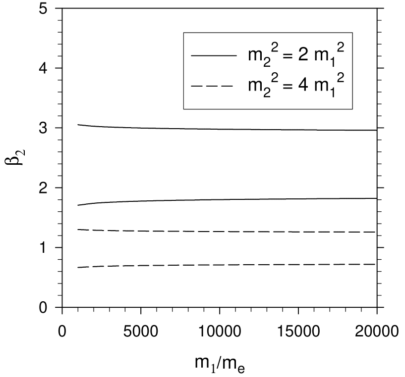
Figure 1: The coupling coefficient $\beta_{2}$ as a function of the PV masses $m_{1}$ and $m_{2}$. The two possible values of $\beta_{2}$ are determined by the constraint of having a zero mass for the physical photon eigenstate. The value used for the bare electron mass $m_{0}$ is $0.99m_{e}$, where $m_{e}$ is the physical electron mass.

The range in $m_{1}$ is taken up to the point where the earlier calculations were done for the dressed-electron state TwoPhotonQED ; the value of $m_{2}$ is fixed in ratio to $m_{1}$. The eventual choices of the root and of the $m_{2}/m_{1}$ ratio will be determined by optimization of the numerical calculation. Ideally, the root and the ratio will not be too large; a large root would mean large couplings for the PV particles, and a large ratio would make $m_{2}$ yet another mass scale in the problem.

The main point here is the existence of values of $m_{2}$ and $\beta_{2}$ for which the mass of the photon eigenstate is zero. Also, since $\beta_{2}=0$ is not a root, the addition of the second PV fermion flavor is necessary to restore the zero mass. For calculations in QED that include a single electron-positron pair in the basis, with no photons in the same Fock state, the analytic results given here provide the value to use for $\beta_{2}$.

IV Summary

We have shown that the addition of a second PV fermion flavor is sufficient to restore the physical photon eigenstate to zero mass. The photon self-energy induced by vacuum polarization is thus not only rendered finite by the PV regularization, but an additional finite correction can also be made by adjusting the coupling coefficients of the PV fermions. For the simplest Fock-state basis, we have computed explicitly the coupling coefficients as functions of the electron’s bare mass and the PV fermion masses; the results are illustrated in Fig. 1.

This analysis provides building blocks necessary for the extension of previous work on the dressed-electron state OnePhotonQED ; TwoPhotonQED to include electron-positron pairs. The complete Lorentz-gauge light-front Hamiltonian (II) has been constructed and the one-photon eigenstate has been investigated in some detail. The issues that remain to be resolved are the vacuum-polarization contribution to charge renormalization and the electron-positron pair contribution to current covariance. There are also technical issues to be addressed, associated with the numerical analysis of the coupled equations of the dressed-electron eigenproblem. The size of the calculation will be larger than the case of two-photon truncation TwoPhotonQED , because the number of PV fermion flavors will be two instead of one, but the size should still be small enough for the calculation to be done.

Appendix A Evaluation of $I(0)$

We evaluate the integral $I(M^{2})$, defined in (35), for the case of $M=0$. The symmetry of the integrand allows us to replace $k_{1}^{2}$ and $k_{2}^{2}$ in the numerator by $k_{\perp}^{2}/2$. The integral over azimuthal angle can be done immediately, to replace $d^{2}k_{\perp}$ by $\pi dk_{\perp}^{2}$. The numerator can be written as

$$(1-2x)^{2}k_{\perp}^{2}/2+k_{\perp}^{2}/2+(m_{i}(1-x)+m_{j}x)^{2}=[m_{i}^{2}(1-x)+m_{j}^{2}x+k_{\perp}^{2}]-x(1-x)[(m_{i}-m_{j})^{2}+2k_{\perp}^{2}].$$ (41)

The first bracket can be dropped, since it cancels the matching bracket in the denominator, leaving an integrand independent of $i$ and $j$, for which the sums over $i$ and $j$ are zero. This reduces the form of $I(0)$ to

$$I(0)=\frac{e_{0}^{2}}{8\pi^{3}}\sum_{ij}(-1)^{i+j}\frac{\beta_{i}\beta_{j}}{m_{e}^{2}}\int dxd^{2}k_{\perp}\frac{(m_{i}-m_{j})^{2}+2k_{\perp}^{2}}{m_{i}^{2}(1-x)+m_{j}^{2}x+k_{\perp}^{2}}.$$ (42)

Further simplification comes from writing $k_{\perp}^{2}=[m_{i}^{2}(1-x)+m_{j}^{2}x+k_{\perp}^{2}]-[m_{i}^{2}(1-x)+m_{j}^{2}x]$ in the numerator and again dropping the first bracket, for the same reason as before.

The expression that we actually integrate is, then

$$I(0)=\frac{e_{0}^{2}}{8\pi^{2}}\sum_{ij}(-1)^{i+j}\beta_{i}\beta_{j}\int\frac{dxdk_{\perp}^{2}}{m_{e}^{4}}\frac{(m_{i}-m_{j})^{2}-2[m_{i}^{2}(1-x)+m_{j}^{2}x]}{(1-x)m_{i}^{2}/m_{e}^{2}+xm_{j}^{2}/m_{e}^{2}+k_{\perp}^{2}/m_{e}^{2}}.$$ (43)

The $k_{\perp}^{2}$ integral yields $\ln[(1-x)m_{i}^{2}/m_{e}^{2}+xm_{j}^{2}/m_{e}^{2}+k_{\perp}^{2}/m_{e}^{2}]$ evaluated at 0 and $\infty$; the sums over $i$ and $j$ eliminate the contributions at the upper limit. The remaining expression is

$$I(0)=\frac{e_{0}^{2}}{8\pi^{2}}\sum_{ij}(-1)^{i+j}\beta_{i}\beta_{j}I_{ij},$$ (44)

with

$$I_{ij}\equiv\int_{0}^{1}\frac{dx}{m_{e}^{2}}\left\{2[m_{i}^{2}(1-x)+m_{j}^{2}x]-(m_{i}-m_{j})^{2}\right\}\ln[(1-x)m_{i}^{2}/m_{e}^{2}+xm_{j}^{2}/m_{e}^{2}].$$ (45)

When $i=j$, the integrand is trivial; when $i\neq j$, we can use the transformation $z=(1-x)m_{i}^{2}/m_{e}^{2}+xm_{j}^{2}/m_{e}^{2}$ to arrive at a simple integral. The final results are

$$I_{ij}=\left\{\begin{array}[]{ll}2\frac{m_{i}^{2}}{m_{e}^{2}}\ln\left(\frac{m_{i}^{2}}{m_{e}^{2}}\right),&i=j\\ \frac{m_{i}^{2}+m_{j}^{2}}{2m_{e}^{2}}-\frac{2m_{i}m_{j}}{m_{e}^{2}}+\frac{m_{i}m_{j}}{m_{j}^{2}-m_{i}^{2}}\left[\frac{m_{i}(m_{j}-2m_{i})}{m_{e}^{2}}\ln\left(\frac{m_{i}^{2}}{m_{e}^{2}}\right)-\frac{m_{j}(m_{i}-2m_{j})}{m_{e}^{2}}\ln\left(\frac{m_{j}^{2}}{m_{e}^{2}}\right)\right],&i\neq j.\end{array}\right.$$ (46)

The form of $I(0)$ is now fully specified.

References

• (1) For reviews of lattice theory, see M. Creutz, L. Jacobs and C. Rebbi, Phys. Rep. 95, 201 (1983); J.B. Kogut, Rev. Mod. Phys. 55, 775 (1983); I. Montvay, ibid59, 263 (1987); A.S. Kronfeld and P.B. Mackenzie, Ann. Rev. Nucl. Part. Sci. 43, 793 (1993); J.W. Negele, Nucl. Phys. A553, 47c (1993); K.G. Wilson, Nucl. Phys. B (Proc. Suppl.) 140, 3 (2005); J.M. Zanotti, PoS LAT2008, 007 (2008). For recent discussions of meson properties and charm physics, see for example C. McNeile and C. Michael [UKQCD Collaboration], Phys. Rev. D 74, 014508 (2006); I. Allison et al. [HPQCD Collaboration], Phys. Rev.  D 78, 054513 (2008).
• (2) M. Burkardt and S. Dalley, Prog. Part. Nucl. Phys.  48, 317 (2002) and references therein; S. Dalley and B. van de Sande, Phys. Rev. D 67, 114507 (2003); D. Chakrabarti, A.K. De, and A. Harindranath, Phys. Rev. D 67, 076004 (2003); M. Harada and S. Pinsky, Phys. Lett. B 567, 277 (2003); S. Dalley and B. van de Sande, Phys. Rev. Lett.  95, 162001 (2005); J. Bratt, S. Dalley, B. van de Sande, and E. M. Watson, Phys. Rev.  D 70, 114502 (2004). For work on a complete light-cone lattice, see C. Destri and H.J. de Vega, Nucl. Phys. B290, 363 (1987); D. Mustaki, Phys. Rev. D 38, 1260 (1988).
• (3) C.D. Roberts and A.G. Williams, Prog. Part. Nucl. Phys. 33, 477 (1994); P. Maris and C.D. Roberts, Int. J. Mod. Phys. E12, 297 (2003); P.C. Tandy, Nucl. Phys. B (Proc. Suppl.) 141, 9 (2005).
• (4) For reviews of light-cone quantization, see M. Burkardt, Adv. Nucl. Phys. 23, 1 (2002); S.J. Brodsky, H.-C. Pauli, and S.S. Pinsky, Phys. Rep. 301, 299 (1998).
• (5) S. D. Glazek and R. J. Perry, Phys. Rev.  D 78, 045011 (2008); S.D. Głazek and J. Mlynik, Phys. Rev. D 74, 105015 (2006), S.D. Głazek, Phys. Rev. D 69, 065002 (2004), S.D. Głazek and J. Mlynik, Phys. Rev. D 67, 045001 (2003); S.D. Głazek and M. Wieckowski, Phys. Rev. D 66, 016001 (2002).
• (6) V. A. Karmanov, J. F. Mathiot, and A. V. Smirnov, Phys. Rev. D 77, 085028 (2008).
• (7) J.P. Vary et al., Phys. Rev. C 81, 035205 (2010).
• (8) S.S. Chabysheva and J.R. Hiller, Phys. Rev. D 81, 074030 (2010).
• (9) S.J. Brodsky, J.R. Hiller, and G. McCartor, Phys. Rev. D 58, 025005 (1998); 60, 054506 (1999); 64, 114023 (2001); Ann. Phys. 296, 406 (2002); 321, 1240 (2006).
• (10) S.J. Brodsky, J.R. Hiller, and G. McCartor, Ann. Phys. 305, 266 (2003).
• (11) S.J. Brodsky, V.A. Franke, J.R. Hiller, G. McCartor, S.A. Paston, and E.V. Prokhvatilov, Nucl. Phys. B 703, 333 (2004).
• (12) S.S. Chabysheva and J.R. Hiller, Phys. Rev. D 79, 114017 (2009).
• (13) S.S. Chabysheva, A nonperturbative calculation of the electron’s anomalous magnetic moment, Ph.D. thesis, Southern Methodist University [ProQuest Dissertations & Theses 3369009, 2009].
• (14) S.S. Chabysheva and J.R. Hiller, Ann. Phys. 325, 2435 (2010).
• (15) W. Pauli and F. Villars, Rev. Mod. Phys. 21, 434 (1949).
• (16) P.A.M. Dirac, Rev. Mod. Phys. 21, 392 (1949).
• (17) G.P. Lepage and S.J. Brodsky, Phys. Rev. D 22, 2157 (1980).
• (18) S.N. Gupta, Proc. Phys. Soc. (London) A63, 681 (1950); K. Bleuler, Helv. Phys. Acta 23, 567 (1950).
• (19) N.N. Bogoliubov and D.V. Shirkov, Introduction to the Theory of Quantized Fields, (Interscience, New York, 1959); S. Schweber, An Introduction to Relativistic Quantum Field Theory, (Harper & Row, New York, 1961); C. Itzykson and J.-B. Zuber, Quantum Field Theory, (McGraw–Hill, New York, 1980).