Tree-Structured Stick Breaking Processes for Hierarchical Data

Abstract

Many data are naturally modeled by an unobserved hierarchical structure. In this paper we propose a flexible nonparametric prior over unknown data hierarchies. The approach uses nested stick-breaking processes to allow for trees of unbounded width and depth, where data can live at any node and are infinitely exchangeable. One can view our model as providing infinite mixtures where the components have a dependency structure corresponding to an evolutionary diffusion down a tree. By using a stick-breaking approach, we can apply Markov chain Monte Carlo methods based on slice sampling to perform Bayesian inference and simulate from the posterior distribution on trees. We apply our method to hierarchical clustering of images and topic modeling of text data.

journalname

, and

1 Introduction

Structural aspects of models are often critical to obtaining flexible, expressive model families. In many cases, however, the structure is unobserved and must be inferred, either as an end in itself or to assist in other estimation and prediction tasks. This paper addresses an important instance of the structure learning problem: the case when the data arise from a latent hierarchy. We take a direct nonparametric Bayesian approach, constructing a prior on tree-structured partitions of data that provides for unbounded width and depth while still allowing tractable posterior inference.

Probabilistic approaches to latent hierarchies have been explored in a variety of domains. Unsupervised learning of densities and nested mixtures has received particular attention via finite-depth trees (Williams, 2000), diffusive branching processes (Neal, 2003a) and hierarchical clustering (Heller and Ghahramani, 2005; Teh et al., 2007). Bayesian approaches to learning latent hierarchies have also been useful for semi-supervised learning (Kemp et al., 2004), relational learning (Roy et al., 2007) and multi-task learning (Daumé III, 2009). In the vision community, distributions over trees have been useful as priors for figure motion (Meeds et al., 2008) and for discovering visual taxonomies (Bart et al., 2008).

In this paper we develop a distribution over probability measures that imbues them with a natural hierarchy. These hierarchies have unbounded width and depth and the data may live at internal nodes on the tree. As the process is defined in terms of a distribution over probability measures and not as a distribution over data per se, data from this model are infinitely exchangeable; the probability of any set of data is not dependent on its ordering. Unlike other infinitely exchangeable models (Neal, 2003a; Teh et al., 2007), a pseudo-time process is not required to describe the distribution on trees and it can be understood in terms of other popular Bayesian nonparametric models.

Our new approach allows the components of an infinite mixture model to be interpreted as part of a diffusive evolutionary process. Such a process captures the natural structure of many data. For example, some scientific papers are considered seminal — they spawn new areas of research and cause new papers to be written. We might expect that within a text corpus of scientific documents, such papers would be the natural ancestors of more specialized papers that followed on from the new ideas. This motivates two desirable features of a distribution over hierarchies: 1) ancestor data (the “prototypes”) should be able to live at internal nodes in the tree, and 2) as the ancestor/descendant relationships are not known a priori, the data should be infinitely exchangeable.

2 A Tree-Structured Stick-Breaking Process

Stick-breaking processes based on the beta distribution have played a prominent role in the development of Bayesian nonparametric methods, most significantly with the constructive approach to the Dirichlet process (DP) due to Sethuraman (1994). A random probability measure $G$ can be drawn from a DP with base measure $\alpha H$ using a sequence of beta variates via:

$$G =\sum^{\infty}_{i=1}\pi_{i}\,\delta_{\theta_{i}} \pi_{i} =\nu_{i}\prod^{i-1}_{i^{\prime}=1}(1-\nu_{i^{\prime}})$$ (1)

$$\theta_{i} \sim H \nu_{i} \sim\textrm{Be}(1,\alpha) \pi_{1} =\nu_{1}.$$

We can view this as taking a stick of unit length and breaking it at a random location. We call the left side of the stick $\pi_{1}$ and then break the right side again at a new place, calling the left side of this new break $\pi_{2}$. If we continue this process of “keep the left piece and break the right piece again” as in Fig. 1a, assigning each $\pi_{i}$ a random value drawn from $H$, we can view this is a random probability measure centered on $H$. The distribution over the sequence ${(\pi_{1},\pi_{2},\cdots)}$ is a case of the GEM distribution (Pitman, 2002), which also includes the Pitman-Yor process (Pitman and Yor, 1997). Note that in Eq. (1) the $\theta_{i}$ are i.i.d. from $H$; in the current paper these parameters will be drawn according to a hierarchical process.

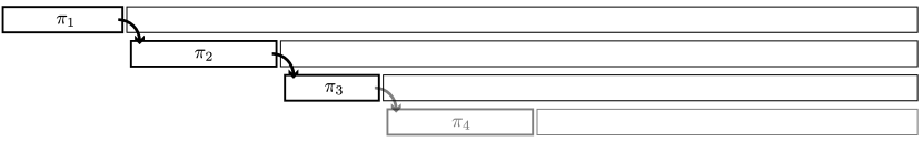
(a) Dirichlet process stick breaking

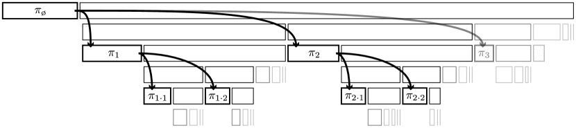
(b) Tree-structured stick breaking

Figure 1: a) Dirichlet process stick-breaking procedure, with a linear partitioning. b) Interleaving two stick-breaking processes yields a tree-structured partition. Rows 1, 3 and 5 are $\nu$-breaks. Rows 2 and 4 are $\psi$-breaks.

The GEM construction provides a distribution over infinite partitions of the unit interval, with natural numbers as the index set as in Fig. 1a. In this paper, we extend this idea to create a distribution over infinite partitions that also possess a hierarchical graph topology. To do this, we will use finite-length sequences of natural numbers as our index set on the partitions. Borrowing notation from the Pólya tree (PT) construction (Mauldin et al., 1992), let ${\boldsymbol{\epsilon}\!=\!(\epsilon_{1},\epsilon_{2},\cdots,\epsilon_{K})}$, denote a length-$K$ sequence of positive integers, i.e., ${\epsilon_{k}\!\in\!\mathbb{N}^{+}}$. We denote the zero-length string as ${\boldsymbol{\epsilon}\!=\!\text{\o}}$ and use $|\boldsymbol{\epsilon}|$ to indicate the length of $\boldsymbol{\epsilon}$’s sequence. These strings will index the nodes in the tree and $|\boldsymbol{\epsilon}|$ will then be the depth of node $\boldsymbol{\epsilon}$.

We interleave two stick-breaking procedures as in Fig. 1b. The first has beta variates ${\nu_{\boldsymbol{\epsilon}}\!\sim\!\textrm{Be}(1,\alpha(|\boldsymbol{\epsilon}|))}$ which determine the size of a given node’s partition as a function of depth. The second has beta variates ${\psi_{\boldsymbol{\epsilon}}\!\sim\!\textrm{Be}(1,\gamma)}$, which determine the branching probabilities. Interleaving these processes partitions the unit interval. The size of the partition associated with each $\boldsymbol{\epsilon}$ is given by

$$\pi_{\boldsymbol{\epsilon}} =\nu_{\boldsymbol{\epsilon}}\varphi_{\boldsymbol{\epsilon}}\prod_{\boldsymbol{\epsilon}^{\prime}\prec\boldsymbol{\epsilon}}\varphi_{\boldsymbol{\epsilon}^{\prime}}(1-\nu_{\boldsymbol{\epsilon}^{\prime}}) \varphi_{\boldsymbol{\epsilon}\epsilon_{i}} =\psi_{i}\prod^{i-1}_{i^{\prime}=1}(1-\psi_{i^{\prime}}) \pi_{\text{\o}} =\nu_{\text{\o}},$$ (2)

where $\boldsymbol{\epsilon}\epsilon_{i}$ denotes the sequence that results from appending $\epsilon_{i}$ onto the end of $\boldsymbol{\epsilon}$, and ${\boldsymbol{\epsilon}^{\prime}\!\prec\!\boldsymbol{\epsilon}}$ indicates that $\boldsymbol{\epsilon}$ could be constructed by appending onto $\boldsymbol{\epsilon}^{\prime}$. When viewing these strings as identifying nodes on a tree, ${\{\boldsymbol{\epsilon}\epsilon_{i}:\epsilon_{i}\!\in\!1,2,\cdots\}}$ are the children of $\boldsymbol{\epsilon}$ and ${\{\boldsymbol{\epsilon}^{\prime}:\boldsymbol{\epsilon}^{\prime}\!\prec\!\boldsymbol{\epsilon}\}}$ are the ancestors of $\boldsymbol{\epsilon}$. The $\{\pi_{\boldsymbol{\epsilon}}\}$ in Eq. (2) can be seen as products of several decisions on how to allocate mass to nodes and branches in the tree: the $\{\varphi_{\boldsymbol{\epsilon}}\}$ determine the probability of a particular sequence of children and the $\nu_{\boldsymbol{\epsilon}}$ and $(1\!-\!\nu_{\boldsymbol{\epsilon}})$ terms determine the proportion of mass allotted to $\boldsymbol{\epsilon}$ versus nodes that are descendants of $\boldsymbol{\epsilon}$.

We require that the $\{\pi_{\boldsymbol{\epsilon}}\}$ sum to one. The $\psi$-sticks have no effect upon this, but ${\alpha(\cdot):\mathbb{N}\to\mathbb{R}^{+}}$ (the depth-varying parameter for the $\nu$-sticks) must satisfy ${\sum_{j\!=\!1}^{\infty}\ln(1\!+\!1/\alpha(j\!-\!1))\!=\!+\infty}$ (see Ishwaran and James (2001)). This is clearly true for $\alpha(j)\!=\!\alpha_{0}\!>\!0$. A useful function that also satisfies this condition is $\alpha(j)\!=\!\lambda^{j}\alpha_{0}$ with $\alpha_{0}\!>\!0,\lambda\!\in\!(0,1]$. The decay parameter $\lambda$ allows a distribution over trees with most of the mass at an intermediate depth. This is the $\alpha(\cdot)$ we will assume throughout the remainder of the paper.

An Urn-based View

When a Bayesian nonparametric model induces partitions over data, it is sometimes possible to construct an urn scheme that corresponds to sequentially generating data, while integrating out the underlying random measure. The “Chinese restaurant” metaphor for the Dirichlet process is a popular example. In our model, we can use such an urn scheme to construct a treed partition over a finite set of data. Note that while the tree illustrated in Fig. 1b is a nested set of size-biased partitions, the ordering of the branches in an urn-based tree over data does not necessarily correspond to a size-biased permutation (Pitman, 1996).

The data drawing process can be seen as a path-reinforcing Bernoulli trip down the tree where each datum starts at the root and descends into children until it stops at some node. The first datum lives at the root node with probability ${1/(\alpha(0)\!+\!1)}$, otherwise it descends and instantiates a new child. It stays at this new child with probability ${1/(\alpha(1)\!+\!1)}$ or descends again and so on. A later datum stays at node $\boldsymbol{\epsilon}$ with probability ${(N_{\boldsymbol{\epsilon}}\!+\!1)/(N_{\boldsymbol{\epsilon}}\!+\!N_{\boldsymbol{\epsilon}\prec\cdot}\!+\!\alpha(|\boldsymbol{\epsilon}|)\!+\!1)}$, where $N_{\boldsymbol{\epsilon}}$ is the number of previous data that stopped at $\boldsymbol{\epsilon}$, and $N_{\boldsymbol{\epsilon}\prec\cdot}$ is the number of previous data that came down this path of the tree but did not stop at $\boldsymbol{\epsilon}$, i.e., a sum over all descendants: ${N_{\boldsymbol{\epsilon}\prec\cdot}\!=\!\sum_{\boldsymbol{\epsilon}\prec\boldsymbol{\epsilon}^{\prime}}N_{\boldsymbol{\epsilon}^{\prime}}}$. If a datum descends to $\boldsymbol{\epsilon}$ but does not stop then it chooses which child to descend to according to a Chinese restaurant process where the previous customers are only those data who have also descended to this point. That is, if it has reached node $\boldsymbol{\epsilon}$ but will not stay there, it descends to existing child $\boldsymbol{\epsilon}\epsilon_{i}$ with probability ${(N_{\boldsymbol{\epsilon}\epsilon_{i}}\!+\!N_{\boldsymbol{\epsilon}\epsilon_{i}\prec\cdot})/(N_{\boldsymbol{\epsilon}\prec\cdot}\!+\!\gamma)}$ and instantiates a new child with probability ${\gamma/(N_{\boldsymbol{\epsilon}\prec\cdot}\!+\!\gamma)}$. A particular path therefore becomes more likely according to its “popularity” with previous data. Note that a node can be a part of a popular path without having any data of its own. Fig. 2h shows the structures implied over fifty data drawn from this process with different hyperparameter settings.

The urn view allows us to place this model into the literature on priors on infinite trees. One of the main contributions of this model is that the data can live at arbitrary internal nodes in the tree, but are nevertheless infinitely exchangeable. This is in contrast to the model proposed by Meeds et al. (2008), for example, which is not infinitely exchangeable. The nested Chinese restaurant process (nCRP) (Blei et al., 2010) provides a distribution over trees of unbounded width and depth, but data correspond to reinforcing paths of infinite length, requiring an additional distribution over depths that is not path-dependent. The Pólya tree (Mauldin et al., 1992) uses a recursive stick-breaking process to specify a distribution over nested partitions in a binary tree, however the resulting data live at the infinitely-deep leaf nodes. The marginal distribution over the topology of a Dirichlet diffusion tree (Neal, 2003a) (and the clustering variant of Kingman’s coalescent proposed by Teh et al. (2007)) provides path-reinforcement and infinite exchangeability, however the topology is determined by a hazard process in pseudo-time and data do not live at internal nodes.

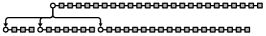
(a) $\alpha_{0}\!=\!1$, $\lambda\!=\!\frac{1}{2}$, $\gamma\!=\!\frac{1}{5}$

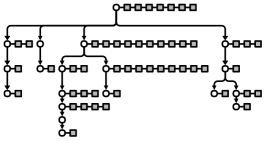
(b) $\alpha_{0}\!=\!1$, $\lambda\!=\!1$, $\gamma\!=\!\frac{1}{5}$

(c) $\alpha_{0}\!=\!1$, $\lambda\!=\!1$, $\gamma\!=\!1$

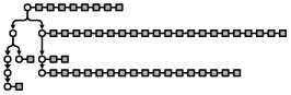
(d) $\alpha_{0}\!=\!5$, $\lambda\!=\!\frac{1}{2}$, $\gamma\!=\!\frac{1}{5}$

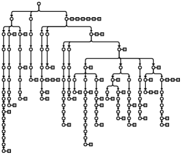
(e) $\alpha_{0}\!=\!5$, $\lambda\!=\!1$, $\gamma\!=\!\frac{1}{5}$

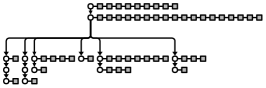
(f) $\alpha_{0}\!=\!5$, $\lambda\!=\!\frac{1}{2}$, $\gamma\!=\!1$

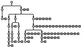
(g) $\alpha_{0}\!=\!25$, $\lambda\!=\!\frac{1}{2}$, $\gamma\!=\!\frac{1}{5}$

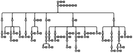
(h) $\alpha_{0}\!=\!25$, $\lambda\!=\!\frac{1}{2}$, $\gamma\!=\!1$

Figure 2: Eight samples of trees over partitions of fifty data, with different hyperparameter settings. The circles are represented nodes, and the squares are the data. Note that some of the sampled trees have represented nodes with no data associated with them and that the branch ordering does not correspond to a size-biased permutation.

3 Hierarchical Priors for Node Parameters

In the stick-breaking construction of the Dirichlet process one can view the procedure as generating an infinite partition and then labeling each cell $i$ with parameter $\theta_{i}$ drawn i.i.d. from $H$. In a mixture model, data that are drawn from the $i$th component are generated independently according to a distribution $f(x\,|\,\theta_{i})$, where $x$ takes values in a sample space $\mathcal{X}$. In our model, we continue to assume that the data are generated independently given the latent labeling, but to take advantage of the tree-structured partitioning of Section 2 an i.i.d. assumption on the node parameters is inappropriate. Rather, the distribution over the parameters at node $\boldsymbol{\epsilon}$, denoted $\theta_{\boldsymbol{\epsilon}}$, should depend in an interesting way on its ancestors ${\{\theta_{\boldsymbol{\epsilon}^{\prime}}:\boldsymbol{\epsilon}^{\prime}\!\prec\!\boldsymbol{\epsilon}\}}$. A natural and powerful way to specify such dependency is via a directed graphical model, with the requirement that edges must always point down the tree. An intuitive subclass of such graphical models are those in which a child is conditionally independent of all ancestors, given its parents and any global hyperparameters. This is the case we will focus on here, as it provides a useful view of the parameter-generation process as a “diffusion down the tree” via a Markov transition kernel that can be essentially any distribution with a location parameter. Coupling such a kernel, which we denote $T(\theta_{\boldsymbol{\epsilon}\epsilon_{i}}\!\leftarrow\!\theta_{\boldsymbol{\epsilon}})$, with a root-level prior $p(\theta_{\text{\o}})$ and the node-wise data distribution $f(x\,|\,\theta_{\boldsymbol{\epsilon}})$, we have a complete model for infinitely exchangeable tree-structured data on $\mathcal{X}$. We now examine a few specific examples.

Generalized Gaussian Diffusions

If our data distribution $f(x\,|\,\theta)$ is such that the parameters can be specified as a real-valued vector $\theta\!\in\!\mathbb{R}^{M}$, then we can use a Gaussian distribution to describe the parent-to-child transition kernel: ${T_{\textsf{norm}}(\theta_{\boldsymbol{\epsilon}\epsilon_{i}}\!\leftarrow\!\theta_{\boldsymbol{\epsilon}})\!=\!\mathcal{N}(\theta_{\boldsymbol{\epsilon}\epsilon_{i}}\,|\,\eta\,\theta_{\boldsymbol{\epsilon}},\Lambda)}$, where ${\eta\!\in\![0,1)}$. Such a kernel captures the simple idea that the child’s parameters are noisy versions of the parent’s, as specified by the covariance matrix $\Lambda$, while $\eta$ ensures that all parameters in the tree have a finite marginal variance. While this will not result in a conjugate model unless the data are themselves Gaussian, it has the simple property that each node’s parameter has a Gaussian prior that is specified by its parent. We present an application of this model in Section 5, where we model images as a distribution over binary vectors obtained by transforming a real-valued vector to $(0,1)$ via the logistic function.

Chained Dirichlet-Multinomial Distributions

If each datum is a set of counts over $M$ discrete outcomes, as in many finite topic models, a multinomial model for $f(x\,|\,\theta)$ may be appropriate. In this case, ${\mathcal{X}\!=\!\mathbb{N}^{M}}$, and $\theta_{\boldsymbol{\epsilon}}$ takes values in the $(M\!-\!1)$-simplex. We can construct a parent-to-child transition kernel via a Dirichlet distribution with concentration parameter $\kappa$: ${T_{\textsf{dir}}(\theta_{\boldsymbol{\epsilon}\epsilon_{i}}\!\leftarrow\!\theta_{\boldsymbol{\epsilon}})\!=\!\textrm{Dir}(\kappa\theta_{\boldsymbol{\epsilon}})}$, using a symmetric Dirichlet for the root node, i.e., ${\theta_{\text{\o}}\!\sim\!\textrm{Dir}(\kappa\boldsymbol{1})}$.

Hierarchical Dirichlet Processes

A very general way to specify the distribution over data is to say that it is a random probability measure drawn from a Dirichlet process. In our case, a very flexible model would say that the data drawn at node $\boldsymbol{\epsilon}$ are from a distribution $G_{\boldsymbol{\epsilon}}$ as in Eq. (1). This means that $\theta_{\boldsymbol{\epsilon}}\sim G_{\boldsymbol{\epsilon}}$ where $\theta_{\boldsymbol{\epsilon}}$ now corresponds to an infinite set of parameters. The hierarchical Dirichlet process (HDP) (Teh et al., 2006) provides a natural parent-to-child transition kernel for the tree-structured model, again with concentration parameter $\kappa$: ${T_{\textsf{hdp}}(G_{\boldsymbol{\epsilon}\epsilon_{i}}\!\leftarrow\!G_{\boldsymbol{\epsilon}})\!=\!\textrm{DP}(\kappa G_{\boldsymbol{\epsilon}})}$. At the top level, we specify a global base measure $H$ for the root node, i.e., ${G_{\text{\o}}\!\sim\!H}$. One negative aspect of this transition kernel is that the $G_{\boldsymbol{\epsilon}}$ will have a tendency to collapse down onto a single atom. One remedy is to smooth the kernel with $\eta$ as in the Gaussian case, i.e., ${T_{\textsf{hdp}}(G_{\boldsymbol{\epsilon}\epsilon_{i}}\!\leftarrow\!G_{\boldsymbol{\epsilon}})\!=\!\textrm{DP}(\kappa\,(\eta\,G_{\boldsymbol{\epsilon}}+(1-\eta)\,H))}$.

4 Inference via Markov chain Monte Carlo

We have so far defined a model for data that are generated from the parameters associated with the nodes of a random tree. Having seen $N$ data points and assuming a model $f(x\,|\,\theta_{\boldsymbol{\epsilon}})$ as in the previous section, we wish to infer possible trees and model parameters. As in most complex probabilistic models, closed form inference is impossible and we instead perform inference by generating posterior samples via Markov chain Monte Carlo (MCMC). To operate efficiently over a variety of regimes without tuning, we use slice sampling (Neal, 2003b) extensively. This allows us to sample from the true posterior distribution over the finite quantities of interest despite the fact that our our model technically contains an infinite number of parameters. The primary data structure in our Markov chain is the set of $N$ strings describing the current assignments of data to nodes, which we denote $\{\boldsymbol{\epsilon}_{n}\}^{N}_{n=1}$. We represent the $\nu$-sticks and parameters $\theta_{\boldsymbol{\epsilon}}$ for all nodes that are traversed by the data in its current assignments, i.e., ${\{\nu_{\boldsymbol{\epsilon}},\theta_{\boldsymbol{\epsilon}}:\exists n,\boldsymbol{\epsilon}\!\prec\!\boldsymbol{\epsilon}_{n}\}}$. We additionally represent all $\psi$-sticks in the “hull” of the tree that contains the data: if at some node $\boldsymbol{\epsilon}$ one of the $N$ data paths passes through child $\boldsymbol{\epsilon}\epsilon_{i}$, then we represent all the $\psi$-sticks in the set ${\bigcup_{\boldsymbol{\epsilon}_{n}}\bigcup_{\boldsymbol{\epsilon}\epsilon_{i}\preceq\boldsymbol{\epsilon}_{n}}\{\psi_{\boldsymbol{\epsilon}\epsilon_{j}}:\epsilon_{j}\!\leq\!\epsilon_{i}\}}$. We also sample from the hyperparameters $\alpha_{0}$, $\gamma$, and $\lambda$ for the tree and any parameters associated with the likelihoods.

function samp-assignment($n$)

  $p_{\sf{slice}}\sim\textrm{Uni}(0,f(x_{n}\,|\,\theta_{\boldsymbol{\epsilon}_{n}}))$

  $u_{\sf{min}}\leftarrow 0$, $u_{\sf{max}}\leftarrow 1$

  loop

    $u\sim\textrm{Uni}(u_{\sf{min}},u_{\sf{max}})$

    $\boldsymbol{\epsilon}\leftarrow$ find-node($u$, ø)

    $p\leftarrow f(x_{n}\,|\,\theta_{\boldsymbol{\epsilon}})$

    if $p>p_{\sf{slice}}$ then return $\boldsymbol{\epsilon}$

    else if $\boldsymbol{\epsilon}\!<\!\boldsymbol{\epsilon}_{n}$ then $u_{\sf{min}}\!\leftarrow\!u$

    else$\;\;u_{\sf{max}}\leftarrow u$       

function find-node($u$, $\boldsymbol{\epsilon}$)

  if $u<\nu_{\boldsymbol{\epsilon}}$ then return $\boldsymbol{\epsilon}$

  else

    $u\leftarrow(u-\nu_{\boldsymbol{\epsilon}})/(1-\nu_{\boldsymbol{\epsilon}})$

    while $u\!<\!1\!-\!\prod_{j}(1\!-\!\psi_{\boldsymbol{\epsilon}\epsilon_{j}})$ do

      Draw a new $\psi$-stick     

    $\boldsymbol{e}\!\leftarrow\!$ edges from $\psi$-sticks

    $i\!\leftarrow\!$ bin index for $u$ from edges

    Draw $\theta_{\boldsymbol{\epsilon}\epsilon_{i}}$ and $\nu_{\boldsymbol{\epsilon}\epsilon_{i}}$ if necessary

    $u\leftarrow(u-e_{i})/(e_{i+1}-e_{i})$

    return find-node($u$, $\boldsymbol{\epsilon}\epsilon_{i}$)   

function size-biased-perm($\boldsymbol{\epsilon}$)

  $\rho\leftarrow\emptyset$

  while represented children do

    $\boldsymbol{w}\leftarrow$ weights from $\{\psi_{\boldsymbol{\epsilon}\epsilon_{i}}\}$

    $\boldsymbol{w}\leftarrow\boldsymbol{w}\backslash\rho$

    $j\sim\boldsymbol{w}$

    $\rho\leftarrow$ append $j$   

  return $\rho$

 

Slice Sampling Data Assignments

The primary challenge in inference with Bayesian nonparametric mixture models is often sampling from the posterior distribution over assignments, as it is frequently difficult to integrate over the infinity of unrepresented components. To avoid this difficulty, we use a slice sampling approach that can be viewed as a combination of the Dirichlet slice sampler of Walker (2007) and the retrospective sampler of Papaspiliopoulos and Roberts (2008).

Section 2 described a path-reinforcing process for generating data from the model. An alternative method is to draw a uniform variate $u$ on $(0,1)$ and break sticks until we know what $\pi_{\boldsymbol{\epsilon}}$ the $u$ fell into. One can imagine throwing a dart at the top of Fig. 1b and considering which $\pi_{\boldsymbol{\epsilon}}$ it hits. We would draw the sticks and parameters from the prior, as needed, conditioning on the state instantiated from any previous draws and with parent-to-child transitions enforcing the prior downwards in the tree. Calling the pseudocode function find-node($u$, $\boldsymbol{\epsilon}$) with ${u\!\sim\!\textrm{Uni}(0,1)}$ and ${\boldsymbol{\epsilon}\!=\!\text{\o}}$ draws such a sample. This provides a retrospective slice sampling scheme on $u$, allowing us to draw posterior samples without having to specify any tuning parameters.

To slice sample the assignment of the $n$th datum, currently assigned to $\boldsymbol{\epsilon}_{n}$, we initialize our slice sampling bounds to $(0,1)$. We draw a new $u$ from the bounds and use the find-node function to determine the associated $\boldsymbol{\epsilon}$ from the currently-represented state, plus any additional state that must be drawn from the prior. We do a lexical comparison (“string-like”) of the new $\boldsymbol{\epsilon}$ and our current state $\boldsymbol{\epsilon}_{n}$, to determine whether this new path corresponds to a $u$ that is “above” or “below” our current state. This lexical comparison prevents us from having to represent the initial $u_{n}$. We shrink the slice sampling bounds appropriately, depending on the result of the comparison, until we find a $u$ whose assignment satisfies the slice. This procedure is given in pseudocode as samp-assignment($n$). After performing this procedure, we can discard any state that is not in the previously-mentioned hull of representation.

Gibbs Sampling Stick Lengths

Given the represented sticks and the current assignments of nodes to data, it is straightforward to resample the lengths of the sticks from the posterior beta distributions

$$\nu_{\boldsymbol{\epsilon}}\,|\,\textrm{data} \sim\textrm{Be}(N_{\boldsymbol{\epsilon}}\!+\!1,N_{\boldsymbol{\epsilon}\prec\cdot}\!+\!\alpha(|\boldsymbol{\epsilon}|))$$

$$\psi_{\boldsymbol{\epsilon}\epsilon_{i}}\,|\,\textrm{data} \sim\textrm{Be}(N_{\boldsymbol{\epsilon}\epsilon_{i}\prec\cdot}\!+\!1,\gamma\!+\!\textstyle{\sum_{j>i}N_{\boldsymbol{\epsilon}\epsilon_{j}\prec\cdot}}),$$

where $N_{\boldsymbol{\epsilon}}$ and $N_{\boldsymbol{\epsilon}\prec\cdot}$ are the path-based counts as described in Section 2.

Gibbs Sampling the Ordering of the $\psi$-Sticks

When using the stick-breaking representation of the Dirichlet process, it is crucial for mixing to sample over possible orderings of the sticks. In our model, we include such moves on the $\psi$-sticks. We iterate over each instantiated node $\boldsymbol{\epsilon}$ and perform a Gibbs update of the ordering of its immediate children using its invariance under size-biased permutation (SBP) (Pitman, 1996). For a given node, the $\psi$-sticks provide a “local” set of weights that sum to one. We repeatedly draw without replacement from the discrete distribution implied by the weights and keep the ordering that results. Pitman (Pitman, 1996) showed that distributions over sequences such as our $\psi$-sticks are invariant under such permutations and we can view the size-biased-perm($\boldsymbol{\epsilon}$) procedure as a Metropolis–Hastings proposal with an acceptance ratio that is always one.

Slice Sampling Stick-Breaking Hyperparameters

Given all of the instantiated sticks, we slice sample from the conditional posterior distribution over the hyperparameters $\alpha_{0}$, $\lambda$ and $\gamma$:

$$p(\alpha_{0},\lambda\,|\,\{\nu_{\boldsymbol{\epsilon}}\}) \propto\mathbb{I}(\alpha^{\sf{min}}_{0}\!<\!\alpha_{0}\!<\!\alpha^{\sf{max}}_{0})\mathbb{I}(\lambda^{\sf{min}}\!<\!\lambda\!<\!\lambda^{\sf{max}})\prod_{\boldsymbol{\epsilon}}\textrm{Be}(\nu_{\boldsymbol{\epsilon}}\,|\,1,\lambda^{|\boldsymbol{\epsilon}|}\alpha_{0})$$

$$p(\gamma\,|\,\{\psi_{\boldsymbol{\epsilon}}\}) \propto\mathbb{I}(\gamma^{\sf{min}}\!<\!\gamma\!<\!\gamma^{\sf{max}})\prod_{\boldsymbol{\epsilon}}\textrm{Be}(\psi_{\boldsymbol{\epsilon}}\,|\,1,\gamma),$$

where the products are over nodes in the aforementioned hull. We initialize the bounds of the slice sampler with the bounds of the top-hat prior.

Selecting a Single Tree

We have so far described a procedure for generating posterior samples from the tree structures and associated stick-breaking processes. If our objective is to find a single tree, however, samples from the posterior distribution are unsatisfying. Following Blei et al. (2010), we report a best single tree structure over the data by choosing the sample from our Markov chain that has the highest complete-data likelihood $p(\{x_{n},\boldsymbol{\epsilon}_{n}\}^{N}_{n=1}\,|\,\{\nu_{\boldsymbol{\epsilon}}\},\{\psi_{\boldsymbol{\epsilon}}\},\alpha_{0},\lambda,\gamma)$.

5 Hierarchical Clustering of Images

We applied our model and MCMC inference to the problem of hierarchically clustering the CIFAR-100 image data set . These data are a labeled subset of the 80 million tiny images dataset (Torralba et al., 2008) with 50,000 ${32\times 32}$ color images. We did not use the labels in our clustering. We modeled the images via 256-dimensional binary features that had been extracted from each image (i.e., $x_{n}\in\{0,1\}^{256}$) using a deep neural network that had been trained for an image retrieval task (Krizhevsky, 2009). We used a factored Bernoulli likelihood at each node, parameterized by a latent 256-dimensional real vector (i.e., $\theta_{\boldsymbol{\epsilon}}\in\mathbb{R}^{256}$) that was transformed component-wise via the logistic function:

$$f(x_{n}\,|\,\theta_{\boldsymbol{\epsilon}}) =\prod_{d=1}^{256}\left(1+\exp\{-\theta^{(d)}_{\boldsymbol{\epsilon}}\}\right)^{-x^{(d)}_{n}}\left(1+\exp\{\theta^{(d)}_{\boldsymbol{\epsilon}}\}\right)^{1-x^{(d)}_{n}}.$$

The prior over the parameters of a child node was Gaussian with its parent’s value as the mean. The covariance of the prior ($\Lambda$ in Section 3) was diagonal and inferred as part of the Markov chain. We placed independent $\textrm{Uni}(0.01,1)$ priors on the elements of the diagonal. To efficiently learn the node parameters, we used Hamiltonian (hybrid) Monte Carlo (HMC) (Duane et al., 1987; Neal, 1993), taking 25 leapfrog HMC steps, with a randomized step size. We occasionally interleaved a slice sampling move for robustness. For the stick-breaking processes, we used ${\alpha_{0}\!\sim\!\textrm{Uni}(10,50)}$, ${\lambda\!\sim\!\textrm{Uni}(0.05,0.8)}$, and ${\gamma\!\sim\!\textrm{Uni}(1,10)}$. Using Python on a single core of a modern workstation each MCMC sweep of the entire model (including slice sampled reassignment of all 50,000 images) requires approximately three minutes. Fig. 3 represents a part of the tree with the best complete-data log likelihood after 4000 iterations. The tree provides a useful visualization of the data set, capturing broad variations in color at the higher levels of the tree, with lower branches varying in texture and shape. A larger version of this tree is provided in the supplementary material.

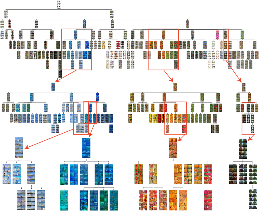
Figure 3: These figures show a subset of the tree learned from the 50,000 CIFAR-100 images. The top tree only shows nodes for which there were at least 250 images. The ten shown at each node are those with the highest probability under the node’s distribution. The second row shows three expanded views of subtrees, with nodes that have at least 50 images. Detailed views of portions of these subtrees are shown in the third row.

6 Hierarchical Modeling of Document Topics

We also used our approach in a bag-of-words topic model, applying it to 1740 papers from NIPS 1–12 . As in latent Dirichlet allocation (LDA) (Blei et al., 2003), we consider a topic to be a distribution over words and each document to be described by a distribution over topics. In LDA, each document has a unique topic distribution. In our model, however, each document lives at a node and that node has a unique topic distribution. Thus multiple documents share a distribution over topics if they inhabit the same node. Each node’s topic distribution is from a chained Dirichlet-multinomial as described in Section 3. The topics each have symmetric Dirichlet priors over their word distributions. This results in a different kind of topic model than that provided by the nested Chinese restaurant process. In the nCRP, each node corresponds to a topic and documents are infinitely-long paths down the tree. Each word is drawn from a distribution over depths that is given by a GEM distribution. In the nCRP, it is not the documents that have the hierarchy, but the topics.

Figure 4: A subtree of documents from NIPS 1-12, inferred using 20 topics. Only nodes with at least 50 documents are shown. Each node shows three aggregated statistics at that node: the five most common author names, the five most common words and a histogram over the years of proceedings.

We did two kinds of analyses. The first is a visualization as with the image data of the previous section, using all 1740 documents. The subtree in Fig. 4 shows the nodes that had at least fifty documents, along with the most common authors and words at that node. The normalized histogram in each box shows which of the twelve years are represented among the documents in that node. An expanded version of this tree is provided in the supplementary material. Secondly, we quantitatively assessed the predictive performance of the model. We created ten random partitions of the NIPS corpus into 1200 training and 540 test documents. We then performed inference with different numbers of topics ($10,20,\ldots,100$) and evaluated the predictive perplexity of the held-out data using an empirical likelihood estimate taken from a mixture of multinomials (pseudo-documents of infinite length, see, e.g. Wallach et al. (2009)) with 100,000 components. As Fig. 5a shows, our model improves in performance over standard LDA for smaller numbers of topics. We believe this improvement is due to the constraints on possible topic distributions that are imposed by the diffusion. For larger numbers of topics, however, it seems that these constraints become a hindrance and the model may be allocating predictive mass to regions where it is not warranted. In absolute terms, more topics did not appear to improve predictive performance for LDA or the tree-structured model. Both models performed best with fewer than fifty topics and the best tree model outperformed the best LDA model on all folds, as shown in Fig. 5b.

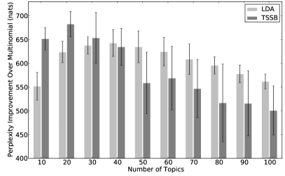
(a) Improvement versus multinomial, by number of topics

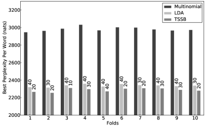
(b) Best perplexity per word, by folds

Figure 5: Results of predictive performance comparison between latent Dirichlet allocation (LDA) and tree-structured stick breaking (TSSB). a) Mean improvement in perplexity per word over Laplace-smoothed multinomial, as a function of topics (larger is better). The error bars show the standard deviation of the improvement across the ten folds. b) Best predictive perplexity per word for each fold (smaller is better). The numbers above the LDA and TSSB bars show how many topics were used to achieve this.

The MCMC inference procedure we used to train our model was as follows: first, we ran Gibbs sampling of a standard LDA topic model for 1000 iterations. We then burned in the tree inference for 500 iterations with fixed word-topic associations. We then allowed the word-topic associations to vary and burned in for an additional 500 iterations, before drawing 5000 samples from the full posterior. For the comparison, we burned in LDA for 1000 iterations and then drew 5000 samples from the posterior (Griffiths and Steyvers, 2004). For both models we thinned the samples by a factor of 50. The mixing of the topic model seems to be somewhat sensitive to the initialization of the $\kappa$ parameter in the chained Dirichlet-multinomial and we initialized this parameter to be the same as the number of topics.

7 Discussion

We have presented a model for a distribution over random measures that also constructs a hierarchy, with the goal of constructing a general-purpose prior on tree-structured data. Our approach is novel in that it combines infinite exchangeability with a representation that allows data to live at internal nodes on the tree, without a hazard rate process. We have developed a practical inference approach based on Markov chain Monte Carlo and demonstrated it on two real-world data sets in different domains.

The imposition of structure on the parameters of an infinite mixture model is an increasingly important topic. In this light, our notion of evolutionary diffusion down a tree sits within the larger class of models that construct dependencies between distributions on random measures (MacEachern, 1999; MacEachern et al., 2001; Teh et al., 2006).

Acknowledgements

The authors wish to thank Alex Krizhevsky for providing the CIFAR-100 binary features; Iain Murray and Yee Whye Teh for valuable advice regarding MCMC inference; Kurt Miller, Hanna Wallach and Sinead Williamson for helpful discussions. RPA is a junior fellow of the Canadian Institute for Advanced Research.

References

- Bart et al. [2008] E. Bart, I. Porteous, P. Perona, and M. Welling. Unsupervised learning of visual taxonomies. In IEEE Conference on Computer Vision and Pattern Recognition, 2008.
- Blei et al. [2003] D. M. Blei, A. Y. Ng, and M. I. Jordan. Latent Dirichlet allocation. Journal of Machine Learning Research, 3:993–1022, 2003.
- Blei et al. [2010] D. M. Blei, T. L. Griffiths, and M. I. Jordan. The nested Chinese restaurant process and Bayesian nonparametric inference of topic hierarchies. Journal of the ACM, 57(2):1–30, 2010.
- Daumé III [2009] H. Daumé III. Bayesian multitask learning with latent hierarchies. In Proceedings of the 25th Conference on Uncertainty in Artificial Intelligence, 2009.
- Duane et al. [1987] S. Duane, A. D. Kennedy, B. J. Pendleton, and D. Roweth. Hybrid Monte Carlo. Physics Letters B, 195(2):216–222, 1987.
- Griffiths and Steyvers [2004] T. L. Griffiths and M. Steyvers. Finding scientific topics. Proceedings of the National Academy of Sciences of the United States of America, 101(Suppl. 1):5228–5235, 2004.
- Heller and Ghahramani [2005] K. A. Heller and Z. Ghahramani. Bayesian hierarchical clustering. In Proceedings of the 22nd International Conference on Machine Learning, 2005.
- Ishwaran and James [2001] H. Ishwaran and L. F. James. Gibbs sampling methods for stick-breaking priors. Journal of the American Statistical Association, 96(453):161–173, March 2001.
- Kemp et al. [2004] C. Kemp, T. L. Griffiths, S. Stromsten, and J. B. Tenenbaum. Semi-supervised learning with trees. In Advances in Neural Information Processing Systems 16. 2004.
- Krizhevsky [2009] A. Krizhevsky. Learning multiple layers of features from tiny images. Technical report, Department of Computer Science, University of Toronto, 2009.
- MacEachern [1999] S. N. MacEachern. Dependent nonparametric processes. In Proceedings of the Section on Bayesian Statistical Science, 1999.
- MacEachern et al. [2001] S. N. MacEachern, A. Kottas, and A. E. Gelfand. Spatial nonparametric Bayesian models. Technical Report 01-10, Institute of Statistics and Decision Sciences, Duke University, 2001.
- Mauldin et al. [1992] R. D. Mauldin, W. D. Sudderth, and S. C. Williams. Pólya trees and random distributions. The Annals of Statistics, 20(3):1203–1221, September 1992.
- Meeds et al. [2008] E. Meeds, D. A. Ross, R. S. Zemel, and S. T. Roweis. Learning stick-figure models using nonparametric Bayesian priors over trees. In IEEE Conference on Computer Vision and Pattern Recognition, 2008.
- Neal [1993] R. M. Neal. Probabilistic inference using Markov chain Monte Carlo methods. Technical Report CRG-TR-93-1, Department of Computer Science, University of Toronto, 1993.
- Neal [2003a] R. M. Neal. Density modeling and clustering using Dirichlet diffusion trees. In Bayesian Statistics 7, pages 619–629, 2003a.
- Neal [2003b] R. M. Neal. Slice sampling (with discussion). The Annals of Statistics, 31(3):705–767, 2003b.
- Papaspiliopoulos and Roberts [2008] O. Papaspiliopoulos and G. O. Roberts. Retrospective Markov chain Monte Carlo methods for Dirichlet process hierarchical models. Biometrika, 95(1):169–186, 2008.
- Pitman [1996] J. Pitman. Random discrete distributions invariant under size-biased permutation. Advances in Applied Probability, 28(2):525–539, 1996.
- Pitman [2002] J. Pitman. Poisson–Dirichlet and GEM invariant distributions for split-and-merge transformation of an interval partition. Combinatorics, Probability and Computing, 11:501–514, 2002.
- Pitman and Yor [1997] J. Pitman and M. Yor. The two-parameter Poisson–Dirichlet distribution derived from a stable subordinator. The Annals of Probability, 25(2):855–900, 1997.
- Roy et al. [2007] D. M. Roy, C. Kemp, V. K. Mansinghka, and J. B. Tenenbaum. Learning annotated hierarchies from relational data. In Advances in Neural Information Processing Systems 19, 2007.
- Sethuraman [1994] J. Sethuraman. A constructive definition of Dirichlet priors. Statistica Sinica, 4:639–650, 1994.
- Teh et al. [2006] Y. W. Teh, M. I. Jordan, M. J. Beal, and D. M. Blei. Hierarchical Dirichlet processes. Journal of the American Statistical Association, 101(476):1566–1581, 2006.
- Teh et al. [2007] Y. W. Teh, H. Daumé III, and D. Roy. Bayesian agglomerative clustering with coalescents. In Advances in Neural Information Processing Systems 20, 2007.
- Torralba et al. [2008] A. Torralba, R. Fergus, and W. T. Freeman. 80 million tiny images: A large data set for nonparametric object and scene recognition. IEEE Transactions on Pattern Analysis and Machine Intelligence, 30(11):1958–1970, 2008.
- Walker [2007] S. G. Walker. Sampling the Dirichlet mixture model with slices. Communications in Statistics, 36:45–54, 2007.
- Wallach et al. [2009] H. M. Wallach, I. Murray, R. Salakhutdinov, and D. Mimno. Evaluation methods for topic models. In Proceedings of the 26th International Conference on Machine Learning, 2009.
- Williams [2000] C. K. I. Williams. A MCMC approach to hierarchical mixture modelling. In Advances in Neural Information Processing Systems 12, pages 680–686. 2000.