Abstract

We reconsider an inflationary model that inflaton field is non-minimally coupled to gravity. We study parameter space of the model up to the second ( and in some cases third ) order of the slow-roll parameters. We calculate inflation parameters in both Jordan and Einstein frames and the results are compared in these two frames and also with observations. Using the recent observational data from combined WMAP5+SDSS+SNIa datasets, we study constraint imposed on our model parameters especially the nonminimal coupling $\xi$.
PACS: 98.80.-k,  98.80.Cq
Key Words: Inflation, Scalar-Tensor Theories, Observational Constraints

1 Introduction

The idea of cosmological inflation is one of the cornerstones of the modern cosmology. It solves the horizon, flatness and monopole problems and provides a mechanism for generation of density perturbations needed to seed the formation of structures in the universe [1-3]. Inflation is believed to be driven by a scalar field that can interact essentially with other fields such as gravity. So, it is natural to include an explicit non-minimal coupling between inflaton and the gravitational sector. However, incorporation of an explicit non-minimal coupling has disadvantage that it is harder to realize inflation even with potentials that are known to be inflationary in the minimal theory [4]. Using the conformal equivalence between gravity theories with minimally and non-minimally coupled scalar fields, for any inflationary model based on a minimally-coupled scalar field, it is possible to construct infinitely many conformally related models with a non-minimal coupling [5,6] ( see also the more recent reference in [7]). Non-minimal coupling is forced upon us from several compelling reasons [4] and a complete theory of cosmological inflation should take into account possible coupling of the inflaton field and the gravitational sector of the theory. There are several comprehensive studies in the field of non-minimal inflation and some severe constraints are imposed on the values that non-minimal coupling ( especially the conformal coupling) can attain in confrontation with observational data [4-7]. Nevertheless, the motivation for present study lies in the fact that there are very limited number of studies that handled the non-minimal inflation up to the second order of the slow-roll parameters and even these limited number of studies have not treated the problem completely ( see for instance [6,7]). On the other hand, the results of calculations for inflation quantities preformed in Jordan and Einstein frames are the same just to first order of the slow-roll parameters [8] and in the second order calculations there may be considerable differences between results of the calculations preformed in these two frames. Our purpose here is to do all of the required calculations up to the second order of the slow-roll parameters in each frames versus the conformal coupling. Then by confronting our results with recent observations from combined WMAP5+SDSS+BAO datasets, we find severe constraint on the values of the non-minimal coupling $\xi$. We also compare the results of calculations in this two frames and in this comparison it is possible to judge about successes of each of these two frames for explanation of the inflation parameters in comparison with observations. Our strategy to perform formal and numerical analysis is to calculate all inflationary parameters up to the second ( in some cases up to the third) order of the slow-roll parameters versus the conformal coupling. A numerical analysis of the model parameter space illuminates the nature of inflationary dynamics of a non-minimally coupled inflaton field up to second order of the slow-roll parameters. Finally a detailed discussion on the issue of frames will be presented.

2 Non-Minimal Inflation in the Jordan Frame

The action of an inflation model where inflaton field is non-minimally coupled to gravity can be expressed as follows

$$S=\int d^{4}x\sqrt{-g}\left[\frac{1}{2\kappa^{2}}R-\frac{1}{2}g^{\mu\nu}\partial_{\mu}\phi\partial_{\nu}\phi+\frac{1}{2}\xi R\phi^{2}+V(\phi)\right].$$ (1)

Variation of this action with respect to the metric leads to the Einstein field equations. If we assume a spatially flat FRW cosmology with line element defined as $ds^{2}=g_{\mu\nu}dx^{\mu}dx^{\nu}=dt^{2}-a^{2}(t)d\vec{x}^{2}$, the Friedmann equation takes the following form

$$H^{2}=\frac{\kappa^{2}}{3(1+\kappa^{2}\xi\phi^{2})}\bigg{[}\frac{1}{2}\dot{\phi}^{2}+V(\phi)-6\xi H\phi\dot{\phi}\bigg{]}.$$ (2)

On the other hand, variation of the action with respect to the scalar field leads to the Klein-Gordon equation of motion [6-8]

$$\ddot{\phi}+3H\dot{\phi}+\bigg{[}\frac{\kappa^{2}\xi\phi^{2}(1+6\xi)}{1+\kappa^{2}\xi\phi^{2}(1+6\xi)}\bigg{]}\frac{\dot{\phi}^{2}}{\phi}=\frac{1}{1+\kappa^{2}\xi\phi^{2}(1+6\xi)}\bigg{[}4\kappa^{2}\xi\phi V(\phi)-(1+\kappa^{2}\xi\phi^{2})V_{,\phi}\bigg{]}.$$ (3)

We note that existence of a negative conformal coupling ( that is, $\xi<0$ ) unavoidably introduces two critical values of the scalar field $\pm\phi_{c}=\pm\frac{1}{\kappa\sqrt{|\xi|}}$,  which are barriers that the scalar field cannot cross. Note also that in these values, the effective gravitational coupling, its gradient, and the total stress-energy tensor diverge [4,9].

The slow-roll conditions are defined as

$$\bigg{|}\frac{\ddot{\phi}}{\dot{\phi}}\bigg{|}\ll H,\quad\quad\bigg{|}\frac{\dot{\phi}}{\phi}\bigg{|}\ll H,\quad\quad\dot{\phi}^{2}\ll V(\phi),\quad\quad\bigg{|}\dot{H}\bigg{|}\ll H^{2}.$$ (4)

By considering the inflation potential of the type $V(\phi)=\lambda\phi^{4}$, the slow-roll conditions give

$$3H\dot{\phi}\approx\frac{-4\lambda\phi^{3}}{1+\kappa^{2}\xi\phi^{2}(1+6\xi)},$$ (5)

and

$$H^{2}\approx\frac{V(\phi)\kappa^{2}}{3(1+\kappa^{2}\xi\phi^{2})}.$$ (6)

In the Jordan frame, the slow-roll parameters which are defined as

$$\epsilon\equiv\frac{-\dot{H}}{H^{2}},\quad\quad\eta\equiv\frac{-\ddot{H}}{H\dot{H}},\quad\quad\zeta\equiv\frac{V^{\prime}\delta\phi}{\dot{\phi}^{2}}=\frac{V^{\prime}H}{2\pi\dot{\phi}^{2}}\,\,,$$ (7)

can be determined as follows

$$\epsilon\simeq\frac{4(2+\kappa^{2}\xi\phi^{2})}{\kappa^{2}\phi^{2}(1+\kappa^{2}\xi\phi^{2}(1+6\xi))}\,\,,$$ (8)

$$\eta\simeq\frac{4(2-\kappa^{2}\xi\phi^{2})}{\kappa^{2}\phi^{2}(2+\kappa^{2}\xi\phi^{2})}$$ (9)

and

$$\zeta\simeq\frac{(3\lambda)^{\frac{1}{2}}}{8\pi\xi^{\frac{3}{2}}}(1+\kappa^{2}\xi\phi^{2}(1+6\xi))^{2}.$$ (10)

During the inflationary phase, each of these slow-roll parameters remains less than unity. Solving for the value of the field at the time of horizon-crossing is difficult in either frame, but following [6], we can use the fact that scales of interest to us crossed outside of the horizon approximately $70$ e-folds before the end of inflation, that is

$$e^{\alpha}\equiv\frac{a(t_{end})}{a(t_{HC})}\sim e^{60},$$ (11)

where HC marks horizon crossing. $\phi_{HC}$ which is needed to evaluate the spectral index $n_{s}$ can be calculated using equation (11). To do this end, we should specify $\phi_{end}$, the value of the Jordan-frame field at the time that inflation ends. As usual, inflation ends when the condition $\epsilon=1$ is fulfilled ( however, we note that it is possible also to fulfill $\eta=1$ even before fulfilling the condition $\epsilon=1$. In this case the condition for exiting from inflation phase is given by $\eta=1$). Setting $\epsilon=1$, we arrive at the condition $\kappa^{2}\xi\phi_{end}^{2}=\beta^{2}(\xi)$ where $\beta$ is given as follows

$$\beta=\bigg{(}\frac{(12\xi-1)+\sqrt{432\xi^{2}+24\xi+1}}{2(1+6\xi)}\bigg{)}^{\frac{1}{2}}.$$ (12)

Now the slow-roll parameters can be expressed just versus the non-minimal coupling as follows

$$\epsilon\simeq\frac{4\xi}{m^{2}}\frac{2+m^{2}}{1+m^{2}(1+6\xi)}\,\,,$$ (13)

$$\eta\simeq\frac{4\xi}{m^{2}}\frac{2-m^{2}}{2+m^{2}}\,\,,$$ (14)

and

$$\zeta\simeq\frac{(3\lambda)^{\frac{1}{2}}}{8\pi\xi^{\frac{3}{2}}}(1+m^{2}(1+6\xi))^{2}\,,$$ (15)

where $m^{2}(\xi)=\kappa^{2}\xi\phi_{HC}^{2}$ and the appropriate $m(\xi)$ can be determined by the initial conditions. Using the definition of $\alpha$ and up to the first order of the non-minimal coupling, in the limit of $m\gg 1$ we find

$$\epsilon\simeq\frac{8\xi}{(16\xi\alpha+1)}\,\,,$$ (16)

$$\eta\simeq\frac{-8\xi}{(3+16\xi\alpha)}\,\,,$$ (17)

and

$$\zeta\simeq\frac{(3\lambda)^{\frac{1}{2}}}{16\pi\xi^{\frac{3}{2}}}(16\xi\alpha+1)^{2}\,.$$ (18)

In this case, the first order ( in the slow-roll parameters) spectral index, $n_{s}=1-6\epsilon+2\eta$ can be written as

$$n_{s}=1-\frac{8}{\kappa^{2}\phi^{2}}\bigg{(}\frac{3(2+\kappa^{2}\xi\phi^{2})}{\big{(}1+\kappa^{2}\xi\phi^{2}(1+6\xi)\big{)}}+\frac{(2-\kappa^{2}\xi\varphi^{2})}{(2+\kappa^{2}\phi^{2})}\bigg{)}$$ (19)

$$n_{s}\simeq 1-\frac{32\xi}{16\xi\alpha-1}\,\,,$$ (20)

where we have used the approximation $\alpha\simeq 60\gg 1$. Up to the second order of the slow-roll parameters, the spectral index $n_{s}$ depends on the three parameters $\epsilon$,  $\eta$  and $\zeta$ in the following manner [6]

$$n_{s}\simeq 1-6\epsilon+2\eta+\frac{1}{3}(44-18c)\epsilon^{2}+(4c-14)\epsilon\eta+\frac{2}{3}\eta^{2}+\frac{1}{6}(13-3c)\zeta^{2}\,,$$ (21)

where $c\equiv 4(\ln 2+\gamma)\simeq 5.081$ with $\gamma\simeq 0.577$. Therefore, the spectral index in the Jordan frame calculated up to the second order of the slow-roll parameters expressed in terms of the non-minimal coupling is as follows

$$n_{s}\simeq 1-6\Big{(}\frac{8\xi}{16\xi\alpha+1}\Big{)}+2\Big{(}\frac{-16\xi}{3+16\xi\alpha}\Big{)}+6.324\Big{(}\frac{8\xi}{16\xi\alpha+1}\Big{)}\Big{(}\frac{-16\xi}{3+16\xi\alpha}\Big{)}$$

$$-15.819\Big{(}\frac{8\xi}{16\xi\alpha+1}\Big{)}^{2}+\frac{2}{3}\Big{(}\frac{-16\xi}{(3+16\xi\alpha)}\Big{)}^{2}$$

$$+0.373\bigg{(}\frac{(3\lambda)^{\frac{1}{2}}}{16\pi\xi^{\frac{3}{2}}}(16\xi\alpha+1)^{2}\bigg{)}^{2}.$$ (22)

Since by definition

$$\alpha_{s}=\frac{dn_{s}}{d\ lnk}=\frac{d\phi}{d\ lnk}\frac{dn_{s}}{d\phi}$$

and

$$\frac{d\ lnk}{d\phi}=\frac{4\pi}{m_{pl}^{2}}\frac{H}{H^{\prime}}(\epsilon-1),$$

the running of the spectral index in the Jordan frame can be calculated using equations (16)-(18) to find

$$\alpha_{s}=14\epsilon\eta-12\epsilon^{2}-2\zeta^{2}-2\Big{(}-18c+\frac{151}{3}\Big{)}\epsilon^{2}\eta-2\Big{(}\frac{-44}{3}+4c\Big{)}\epsilon\eta^{2}$$

$$-5\Big{(}c-\frac{11}{3}\Big{)}\epsilon\zeta^{2}-\frac{1}{2}\Big{(}7-c\Big{)}\eta\zeta^{2}-\frac{4}{3}\Big{(}44-18c\Big{)}\epsilon^{3}.$$ (23)

The amplitude of the scalar perturbation is defined as

$$P_{s}(k)=\frac{k^{3}}{2\pi^{2}}\frac{H^{2}}{\dot{\phi}^{2}}\big{|}\delta\phi_{k}\big{|}^{2}\equiv A_{s}^{2}\bigg{(}\frac{k}{aH}\bigg{)}^{n_{s}-1},$$ (24)

where

$$A_{s}^{2}=\frac{1}{2\pi^{2}}\bigg{(}\frac{H^{2}}{\dot{\phi}}\bigg{)}^{2}.$$ (25)

The amplitude of the tensor perturbations at the Hubble crossing are given by

$$A_{T}^{2}=\frac{8}{m_{pl}^{2}}\bigg{(}\frac{H}{2\pi}\bigg{)}^{2}.$$ (26)

Therefore, the tensor-to-scalar ratio in our setup is given by

$$r=16\frac{A_{T}^{2}}{A_{s}^{2}}=\frac{128}{\kappa^{2}\phi^{2}}\frac{(1+\kappa^{2}\xi\phi^{2})^{2}}{\big{(}1+\kappa^{2}\xi\phi^{2}(1+6\xi)\big{)}^{2}}\,\,,$$ (27)

where transform to the following form

$$r\simeq\frac{256\xi}{(16\xi\alpha-1)(1+6\xi)}.$$ (28)

Finally, the number of e-folds in Jordan frame is defined as follows

$$N=\int_{\phi_{i}}^{\phi_{end}}\frac{H}{\dot{\phi}}d\phi=-\frac{1}{4}\int_{\phi_{i}}^{\phi_{end}}\frac{\phi[1+\kappa^{2}\xi\phi^{2}(1+6\xi)]}{1+\kappa^{2}\xi\phi^{2}}d\phi.$$ (29)

Since $\kappa^{2}\xi\phi^{2}\gg 1$, this integral can be calculated to find

$$N\approx\frac{\kappa^{2}(1+6\xi)}{8}(\phi_{i}^{2}-\phi_{end}^{2}).$$

In a viable inflation scenario, we can neglect $\phi_{end}^{2}$ in comparison with $\phi_{i}^{2}$. So we find

$$N\approx\frac{\kappa^{2}(1+6\xi)}{8}\phi_{i}^{2}.$$

Most of the inflationary models give $N\geq 60$. With this number of e-folds, one can find an estimation of the value of $\phi_{i}$ if the value of $\xi$ is given. If we consider $0.0003\leq\xi\leq 0.166$ ( will be discussed later), we find $\phi_{i}\geq 22M_{pl}$ in our setup.

We note that for a minimally coupled $(\xi=0)$ spectral index and the tensor-to-scaler ratio are calculated in the standard manner:

$$n_{s}=1-\frac{2}{\alpha}\,\,\,\,,\,\,\,\,r=1-\frac{16}{\alpha}\,\,\,\,.$$ (30)

In the next section we repeat all of the above calculations now in the Einstein frame.

3 The Analysis in the Einstein Frame

Now we reconsider the previous analysis but now in the Einstein frame. We adopt the following conformal transformation

$$\hat{g}_{\mu\nu}=\Omega g_{\mu\nu}\,\,\,\,\,\,,\,\,\,\,\,\,\Omega\equiv 1+\kappa^{2}\xi\phi^{2},$$ (31)

where we use a hat on variables defined in the Einstein frame. With this conformal transformation, we find

$$S=\int d^{4}x\sqrt{-\hat{g}}\ \bigg{[}\frac{1}{2\kappa^{2}}\hat{R}-\frac{1}{2}F^{2}(\phi)\hat{g}^{\mu\nu}\partial_{\mu}\phi\partial_{\nu}\phi+\hat{V}(\phi)\bigg{]},$$ (32)

where by definition

$$F^{2}(\phi)\equiv\frac{1+\kappa^{2}\xi\phi^{2}(1+6\xi)}{(1+k^{2}\xi\phi^{2})^{2}}$$ (33)

and

$$\hat{V}(\hat{\phi})\equiv\frac{V(\phi)}{(1+\kappa^{2}\xi\phi^{2})^{2}}\,.$$ (34)

We transform our coordinate system so that

$$\hat{a}=\sqrt{\Omega}a\,\,\,\,\,\,\,\,\,,\,\,\,\,d\hat{t}=\sqrt{\Omega}dt,$$ (35)

and in this case the metric takes the usual Friedmann-Robertson-Walker form

$$d\hat{s}^{2}=d\hat{t}^{2}-\hat{a}^{2}(\hat{t})d\vec{x}^{2}.$$ (36)

The physical quantities in the Einstein frame should be defined in this coordinate system. The field equations in this frame are given as follows

$$\hat{H}^{2}=\frac{\kappa^{2}}{3}\bigg{[}\Big{(}\frac{d\hat{\phi}}{d\hat{t}}\Big{)}^{2}+\hat{V}(\hat{\phi})\bigg{]},\quad\quad\quad\frac{d^{2}\hat{\phi}}{d\hat{t}^{2}}+3\hat{H}\frac{d\hat{\phi}}{d\hat{t}}+\frac{d\hat{V}}{d\hat{\phi}}=0,$$ (37)

where

$$\hat{H}\equiv\frac{1}{\hat{a}}\frac{d\hat{a}}{d\hat{t}}\frac{1}{\sqrt{\Omega}}\Big{(}H+\frac{1}{2}\frac{\dot{\Omega}}{\Omega}\Big{)},\quad\quad\frac{d\hat{\phi}}{d\hat{t}}\equiv\Big{(}\frac{d\hat{\phi}}{d\phi}\Big{)}\Big{(}\frac{dt}{d\hat{t}}\Big{)}\dot{\phi}=\frac{\sqrt{1+\kappa^{2}\xi\phi^{2}(1+6\xi)}}{\Omega^{\frac{3}{2}}}\dot{\phi}\,\,.$$ (38)

Under the slow-roll approximations $\dot{\hat{\phi}}^{2}\ll\hat{V}$ and $\ddot{\hat{\phi}}\ll 3\hat{H}\dot{\hat{\phi}}$, we find

$$\hat{H}^{2}=\frac{\kappa^{2}}{3}\hat{V}(\hat{\phi}),\quad\quad\quad 3\hat{H}\frac{d\hat{\phi}}{d\hat{t}}+\frac{d\hat{V}}{d\hat{\phi}}=0,$$ (39)

respectively. We define the slow-roll parameters in the Einstein frame as $\hat{\epsilon}\equiv\frac{1}{2\kappa^{2}}\Big{(}\frac{\hat{V}^{\prime}(\hat{\phi})}{\hat{V}(\hat{\phi})}\Big{)}^{2}$,  $\hat{\eta}\equiv\frac{1}{\kappa^{2}}\Big{(}\frac{{\hat{V}}^{\prime\prime}(\hat{\phi})}{\hat{V}(\hat{\phi})}\Big{)}$  and $\hat{\zeta}\equiv\frac{1}{\kappa^{2}}\Big{(}\frac{\hat{V}^{\prime}(\hat{\phi}){\hat{V}}^{\prime\prime}(\phi)}{\hat{V}(\hat{\phi})}\Big{)}$, where a prime marks the differentiation with respect to $\hat{\phi}$. For $V(\phi)=\lambda\phi^{4}$  as the inflaton potential and suitable transformations as mentioned above, we find ( see also [6])

$$\hat{\epsilon}=\frac{8}{\kappa^{2}\phi^{2}\Big{(}1+\kappa^{2}\xi\phi^{2}(1+6\xi)\Big{)}},$$ (40)

and

$$\hat{\eta}=\frac{12\phi^{-2}(1+\kappa^{2}\xi\phi^{2})}{\kappa^{2}\Big{(}1+\kappa^{2}\xi\phi^{2}(1+6\xi)\Big{)}}-\frac{4\kappa^{2}\xi(1+6\xi)(1+\kappa^{2}\xi\phi^{2})}{\Big{(}1+\kappa^{2}\xi\phi^{2}(1+6\xi)\Big{)}^{2}}-\frac{16\kappa^{2}\xi}{\Big{(}1+\kappa^{2}\xi\phi^{2}(1+6\xi)\Big{)}}.$$ (41)

If we write $\kappa^{2}\xi\phi_{HC}^{2}=m^{2}(\xi)$, then the slow-roll parameters can be rewritten as follows

$$\hat{\epsilon}=\frac{8\xi}{m^{2}(1+m^{2}(1+6\xi))},$$ (42)

$$\hat{\eta}=4\xi\frac{3+m^{2}(1+12\xi)-2m^{4}(1+6\xi)}{m^{2}(1+m^{2}(1+6\xi))^{2}},$$ (43)

and

$$\hat{\zeta}=4\sqrt{2}\xi\frac{|3+2m^{2}(-2+3\xi)-15m^{4}(1+6\xi)-6m^{6}(1+6\xi)^{2}+2m^{8}(1+6\xi)^{2}|^{\frac{1}{2}}}{m^{2}(1+m^{2}(1+6\xi))^{2}}$$ (44)

respectively. These equations can be rewritten in terms of $\xi$ and $\alpha$ as follows

$$\hat{\epsilon}=\frac{32\xi}{(16\xi\alpha-1)(16\xi\alpha+1)}\,,$$ (45)

$$\hat{\eta}\simeq\frac{-16\xi}{16\xi\alpha-1}\,,$$ (46)

$$\hat{\zeta}\simeq\frac{16\xi}{16\xi\alpha-1}$$ (47)

respectively. The first order result, $\hat{n}_{s}=1-6\hat{\epsilon}+2\hat{\eta}$, can be approximated in the limit of $m\gg 1$ to find

$$\hat{n_{s}}\simeq 1-\frac{16\xi}{m^{2}(1+6\xi)},$$ (48)

which can be rewritten as follows

$$\hat{n_{s}}\simeq 1-\frac{32\xi}{16\xi\alpha-1}.$$ (49)

The spectral index to the second order in this frame can be obtained as follows

$$\hat{n}_{s}\simeq 1-\frac{48\xi}{m^{4}(1+6\xi)}-\frac{16\xi}{m^{2}(1+6\xi)}-15.819\frac{64\xi^{2}}{m^{8}(1+6\xi)^{2}}+6.324\frac{-64\xi^{2}}{m^{6}(1+6\xi)^{2}}$$

$$+\frac{128}{3}\frac{\xi^{2}}{m^{4}(1+6\xi)^{2}}+0.373\frac{64\xi^{2}}{m^{4}(1+6\xi)^{2}}$$ (50)

On the other hand, the second order result for $n_{s}$ can be approximated in the limit of $m\gg 1$ to find

$$\hat{n}_{s}\simeq 1-6\Big{(}\frac{32\xi}{(16\xi\alpha-1)(16\xi\alpha+1)}\Big{)}+2\Big{(}\frac{-16\xi}{16\xi\alpha-1}\Big{)}+6.324\Big{(}\frac{32\xi}{(16\xi\alpha-1)(16\xi\alpha+1)}\Big{)}\Big{(}\frac{-16\xi}{-1+16\xi\alpha}\Big{)}$$

$$-15.819\Big{(}\frac{32\xi}{(16\xi\alpha-1)(16\xi\alpha+1)}\Big{)}^{2}+\frac{2}{3}\Big{(}\frac{-16\xi}{(-1+16\xi\alpha)}\Big{)}^{2}$$

$$+0.373\bigg{(}\frac{16\xi}{16\xi\alpha-1}\bigg{)}^{2}\,\,.$$ (51)

The running of the spectral index in the Einstein frame in our setup is given by

$$\hat{\alpha}_{s}=14\hat{\epsilon}\hat{\eta}-12\hat{\epsilon}^{2}-2\hat{\zeta}^{2}-2(-18c+\frac{151}{3})\hat{\epsilon}^{2}\hat{\eta}-2(\frac{-44}{3}+4c)\hat{\epsilon}\hat{\eta}^{2}$$

$$-5(c-\frac{11}{3})\hat{\epsilon}\hat{\zeta}^{2}-\frac{1}{2}(7-c)\hat{\eta}\hat{\zeta}^{2}-\frac{4}{3}(44-18c)\hat{\epsilon}^{3}.$$ (52)

This relation can be translated to the following expression

$$\hat{\alpha}_{s}=14\bigg{(}\frac{32\xi}{(16\xi\alpha-1)(16\xi\alpha+1)}\bigg{)}(\frac{-16\xi}{16\xi\alpha-1})-12\bigg{(}\frac{32\xi}{(16\xi\alpha-1)(16\xi\alpha+1)}\bigg{)}^{2}-2(\frac{16\xi}{16\xi\alpha-1})^{2}$$

$$-2(-18c+\frac{151}{3})\bigg{(}\frac{32\xi}{(16\xi\alpha-1)(16\xi\alpha+1)}\bigg{)}^{2}(\frac{-16\xi}{16\xi\alpha-1})-2(\frac{-44}{3}+4c)\bigg{(}\frac{32\xi}{(16\xi\alpha-1)(16\xi\alpha+1)}\bigg{)}$$

$$(\frac{-16\xi}{16\xi\alpha-1})^{2}-5(c-\frac{11}{3})\bigg{(}\frac{32\xi}{(16\xi\alpha-1)(16\xi\alpha+1)}\bigg{)}(\frac{16\xi}{16\xi\alpha-1})^{2}-\frac{1}{2}(7-c)(\frac{-16\xi}{16\xi\alpha-1})(\frac{16\xi}{16\xi\alpha-1})^{2}$$

$$-\frac{4}{3}(44-18c)\bigg{(}\frac{32\xi}{(16\xi\alpha-1)(16\xi\alpha+1)}\bigg{)}^{3}.$$ (53)

The tensor-to-scalar ratio in the Einstein frame is given as follows

$$\hat{r}=16\frac{\hat{A_{T}^{2}}}{\hat{A_{R}^{2}}}\simeq\frac{512\xi}{(16\xi\alpha-1)(16\xi\alpha+1)}\,\,.$$ (54)

Finally, the number of e-folds in the Einstein frame is given by

$$\hat{N}=\int_{\hat{\phi}_{i}}^{\hat{\phi}_{end}}\bigg{(}\frac{\hat{H}}{\dot{\hat{\phi}}}\bigg{)}d\hat{\phi}.$$ (55)

After construction of the mathematical framework, in the next section we study outcomes of this setup in a numerical procedure.

4 Numerical Analysis: Comparison with Observations

Table $1$ gives a comparison between our numerical results in two frames and also in two different order of approximations. The combined WMAP5+SDSS+BAO maximum likelihood (ML) value of $n_{s}$ is given by $n_{s}^{(ML)}=0.962$, while the combined WMAP5+SDSS+BAO mean value (MV) is given by $n_{s}^{(MV)}=0.960\pm 0.013$  [10]. Obviously, the second order results have better agreement with ML result and all results lie in the range of the mean values. We note that in the construction of this table we have used the COBE normalization to find the appropriate value of $\lambda$ so that

$$\bigg{(}\frac{\lambda}{\xi^{2}}\bigg{)}^{\frac{1}{2}}\approx\frac{1}{2}\bigg{(}\frac{\delta\rho}{\rho}\bigg{)}_{hor}=\bigg{(}\frac{\delta T}{T}\bigg{)}_{rms}=1.1\times 10^{-5}$$ (56)

which by adopting the conformal coupling, $\xi=\frac{1}{6}$, gives $\lambda\approx 3.4\times 10^{-12}$. Table $2$ compares the values of the running of the spectral index in two different frames and also in two different order of approximations. Our analysis shows that this non-minimal model generally gives negative values of the running of the spectral index. Also, up to the second order of the slow-roll parameters, the values of the running of the spectral index in the Jordan frame are larger than the values of corresponding quantity in the Einstein frame. Table $3$ compares the values of the tensor-to-scalar ratio in two frames and also in different order of approximations. The value of $r$ in the Jordan frame is more close to observational result than the corresponding result in the Einstein frame.

Table 1: Constraining the non-minimal inflation with WMAP5: The Spectral Index

	$n_{s}(First\,\,order)$	$n_{s}(Second\,\,order)$
$Einstein\,\,Frame$	$0.966$	$0.964$
$Jordan\,\,Frame$	$0.966$	$0.960$
$WMAP5+SDSS+BAO\,\,Mean\,\,Value$	$0.960\pm 0.013$	$---$
$WMAP5+SDSS+BAO\,\,\,ML$	$0.962$	$---$

Table 2: Constraining the non-minimal inflation with WMAP5: The Running of the Spectral Index

	$\alpha_{s}(First\,\,order)$	$\alpha_{s}(Second\,\,order)$
$Einstein\,\,Frame$	$-1.7\times 10^{-3}$	$-0.015$
$Jordan\,\,Frame$	$-1.7\times 10^{-3}$	$-0.013$
$WMAP5+SDSS+BAO\,\,MV$	$-0.068<dn_{s}/d\ln k<0.012$	$---$

Table 3: Constraining the non-minimal inflation with WMAP5: Tensor-to-Scalar Ratio

	$r$
$Einstein\,\,Frame$	$0.003$
$Jordan\,\,Frame$	$0.134$
$WMAP5+SDSS+BAO\,\,MV$	$r<0.22$

Figure $1$ shows the variation of the slow-roll parameter $\epsilon$ versus $\xi$ in two frames. Obviously, in the presence of the non-minimal coupling, natural exit from the inflation phase is achieved without any additional mechanism.

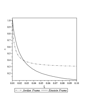
Figure 1: Comparison of two frames. In the presence of the non-minimal coupling, natural exit from inflation phase is possible without any additional mechanism. We have used those values of $\xi$ which are supported by recent observations [11].

Figure $2$ shows the variation of the spectral index versus $\xi$ in the first and second order of the slow-roll parameters in the Jordan frame. Generally, the second order results are more reliable than the first order one in comparison with observation.

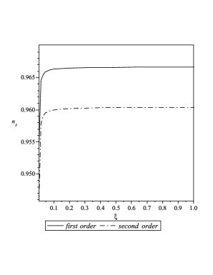
Figure 2: Variation of the spectral index versus $\xi$ in the first and second order of the slow-roll parameters in the Jordan frame.

Figure $3$ shows the variation of the spectral index versus $\xi$ in the first and second order of the slow-roll parameters in the Einstein frame. Once again, the second order results for large values of $\xi$ are more reliable than the first order one in comparison with observation.

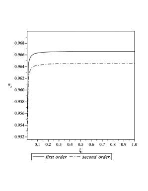
Figure 3: Variation of the spectral index versus $\xi$ in the first and second order of the slow-roll parameters in the Einstein frame.

Figure $4$ shows the variation of $n_{s}$ up to the second order of the slow-roll parameters in two frames. As this figure shows, the values of the $n_{s}$ in the Jordan frame for large values of $\xi$ are closer to observational data.

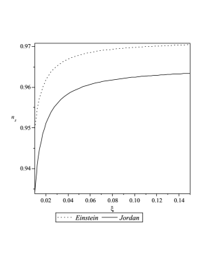
Figure 4: Variation of $n_{s}$ up to the second order of the slow-roll parameters in two frames.

Figure $5$ shows the running of the spectral index up to the second order of the slow-roll parameters in two frames. As this figure shows, the values of the $\alpha_{s}$ in the Jordan frame for large values of $\xi$ are closer to observational data.

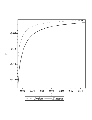
Figure 5: The running of the spectral index up to the second order of the slow-roll parameters in two frames.

5 Remarks on the Issue of Frames

Although our analysis shows good agreements to the observational data and automatic exit from the inflationary era in two frames, but there are some differences in the results of calculations performed in these two frames. Therefore, it is required to discuss about possible fundamental physical meanings of each conformal frame and the physical nature of differences. Since the two frames show considerable differences between their results ( at least in the second order calculations), they are not equivalent in some sense. Then the important question arises: what frame is physically correct for the description of the inflation? On the other hand, the Jordan frame presents a variable effective gravitational constant , while the Einstein frame fixes the gravitational constant. The differences related to the gravitational constant may lead to different interpretations of the nature of the inertia and gravitation. In which follows we address the above issues briefly: The Jordan and Einstein frames are equivalent at the classical level, provided that the units of mass, length, time, and quantities derived there from scale with appropriate powers of the conformal factor in the Einstein frame. What one measures is always the ratio of a quantity to its units, which is the same in the two frames. In the Jordan frame, the units are fixed and in the Einstein frame they vary with the spacetime points. In the Jordan frame the gravitational constant, $G$, is variable, in the Einstein frame it is fixed (but now the units are changed)[13,14]. At the quantum level, the two frames may be inequivalent. If we regard the conformal transformation as a sort of canonical transformation, then Hamiltonians that are classically equivalent (i.e., related by a canonical transformation) are inequivalent when quantized: they have different eigenfunctions and spectra of eigenvalues. So, it is natural that the two frames are inequivalent at the quantum level [14,15].

However, in this paper we are interested in the semiclassical regime. We have computed the spectra of inflationary perturbations, so there will be tensor and scalar fluctuations around a classical background. In this semiclassical case, the two frames should be inequivalent and the spectra (but not amplitudes) of inflationary perturbations computed in the two frames turned out to be the same in certain scenarios of inflation, to first order, but not to second order ( see for instance [6]). As we have noticed in the literature and also by private communications [15], it seems that it is easier to compute fluctuations in the Einstein frame. There is also the issue that, when we want to do a covariant quantization of the Brans-Dicke-like scalar field, we can do it in the Einstein frame but nobody has been able to do it in the Jordan frame [15].

In summary we can say that it seems that the Einstein frame is preferred over the Jordan one at the semiclassical level studied here. In some situations and to the first order, the two frames may still be equivalent. Based on our calculations it seems that at the second (and higher ) order, the two frames are inequivalent. Nevertheless, the calculations in the Einstein frame are much easier.

6 Summary

It is well-known that the results of calculations for inflation quantities preformed in the Jordan and Einstein frames are the same just to the first order of the slow-roll parameters. In the second order calculations, there are considerable differences between results of the calculations preformed in these two frames. In this paper, we have studied a non-minimal inflation with calculations performed up to the second order of the slow-roll parameters versus the conformal coupling explicitly. Then we have compared our results in two frames and also in two order of approximations. On the other hand, by confronting these results with recent observations from combined WMAP5+SDSS+BAO dataset, it is possible to see the differences between two frames and two order of approximations in this setup. Our analysis here shows that in the presence of the non-minimal coupling, natural exit from inflation phase is possible without adopting any additional mechanism. The second order results have generally better agreement with WMAP5+SDSS+BAO ML result and all calculated results lie in the range of the mean values. Our analysis shows also that this non-minimal model generally gives negative values of the running of the spectral index. Up to the second order of the slow-roll parameters, the value of the running of the spectral index in the Jordan frame is larger than the values of the corresponding quantity in the Einstein frame. As our numerical analysis shows, the second order results for large values of $\xi$ are more reliable than the first order one in comparison with observation. The values of the $n_{s}$ in the Jordan frame for large values of $\xi$ are more acceptable in comparison with ML observational data. From another view point we can use observational constraints on the values of, for instance, $n_{s}$ to obtain a constraint on the values of the non-minimal coupling $\xi$. Our calculation up to the second order of the slow-roll parameters for $n_{s}$ in the Jordan frame confronted with observation gives the constraint $0.0003\leq\xi\leq 0.1666$. Nevertheless, we should stress that for $V(\phi)\propto\phi^{4}$, viable cosmological models exist even for $\xi\gg 1$, see for instance [12].

In summary, in this paper the inflationary parameters of a non-minimal inflation model are constrained by the observational data and expressed in terms of the conformal coupling parameter, which plays a fundamental role in the all of our calculations and also suffers strong constraints from the observations on its possible values. The analysis up to the second order of the slow-roll parameters shows that there exist significative differences between the results obtained in two conformally related frames, and this is not the case for the first order approximations. Our study shows that the results provided by the second order calculations present better agreements to the observational data than the first order. As an important result, we have verified that the non-minimally coupled inflationary model can provide automatic exit from the inflationary period without the need to any extra mechanisms.

Acknowledgement

We would like to thank Professor Valerio Faraoni for his invaluable comments on this work. In fact, the section $5$ of the present manuscript is written based on a private communication with him. Also we would like to thank an anonymous referee for his/her critical comments on this work.

References

- [1] A. Liddle and D. Lyth, Cosmological Inflation and Large-Scale Structure, Cambridge University Press, 2000.
- [2] R. H. Brandenberger, [arXiv:hep-th/0509099]; J. E. Lidsey et al, Rev. Mod. Phys. 69 (1997) 373
- [3] A. Riotto, [arXiv:hep-ph/0210162]
- [4] V. Faraoni, Phys. Rev. D 53 (1996) 6813; V. Faraoni, Phys. Rev. D 62 (2000) 023504 ; V. Faraoni, [ arXiv:gr-qc/9807066]
- [5] B. L. Spokoiny, Phys. Lett. B 147 (1984) 39; T. Futamase and K. I. Maeda, Phys. Rev. D 39 (1989) 399; D. S. Salopek, J. R. Bond and J. M. Bardeen, Phys. Rev. D 40 (1989) 1753; R. Fakir and W. G. Unruh, Phys. Rev. D 41 (1990) 1783; C. Schimd, J. P. Uzan and A. Riazuelo, Phys. Rev. D 71 (2005) 083512; N. Makino and M. Sasaki, Prog. Theor. Phys. 86 (1991) 103; R. Fakir, S. Habib and W. G. Unruh, Astrophys. J. 394 (1992) 396; M. V. Libanov, V. A. Rubakov and P. G. Tinyakov, Phys. Lett. B 442 (1998) 63; J. Hwang and H. Noh, Phys. Rev. D 60 (1999) 123001; J. Hwang and H. Noh, Phys. Rev. Lett. 81 (1998) 5274, [arXiv:astro-ph/9811069]; S. Tsujikawa, K. Maeda and T. Torii, Phys. Rev. D60 (1999) 063515; S. Tsujikawa, K. Maeda and T. Torii, Phys. Rev. D60 (1999) 123505; S. Tsujikawa, Phys. Rev. D 62 (2000) 043512; T. Chiba and M. Yamaguchi, Phys. Rev. D 61 (2000) 027304; S. Tsujikawa and H. Yajima, Phys. Rev. D 62 (2000) 123512; E. Gunzig, A. Saa, L. Brenig, V. Faraoni, T. M. Rocha Filho and A. Figueiredo, Phys. Rev. D 63 (2001) 067301 ; S. Koh, S. P. Kim and D. J. Song, Phys. Rev. D 72 (2005) 043523; F. Di Marco and A. Notari, Phys. Rev. D 73 (2006) 063514; M. Bojowald and M. Kagan, Phys. Rev. D 74 (2006) 044033; K. Nozari and B. Fazlpour, JCAP 11 (2007) 006; F. Bauer and D. A. Demir, Phys. Lett. B665 (2008) 222; K. Nozari and B. Fazlpour, [arXiv:0906.5047]; D. A. Easson and R. Gregory, Phys. Rev. D 80 (2009) 083518; M. P. Hertzberg, [ arXiv:1002.2995]; C. Pallis, [ arXiv:1002.4765].
- [6] D. I. Kaiser, Phys. Rev. D 52 (1995) 4295
- [7] T. Chiba and M. Yamaguchi, JCAP 0810 (2008) 021, [arXiv:0807.4965].
- [8] E. Komatsu and T. Futamase, Phys. Rev. D 59 (1999) 064029.
- [9] A. A. Starobinsky, Sov. Astron. Lett. 7 (1981) 36.
- [10] E. Komatsu et al., Astrophys. J. Suppl. 180 (2009) 330 ,[arxive:0803.0547]
- [11] M. Szydlowski, O. Hrycyna and A. Kurek, Phys. Rev. D 77 (2008) 027302, [arXiv:0710.0366]. See also K. Nozari and S. D. Sadatian, Mod. Phys. Lett. A 23(2008) 2933, [arXiv:0710.0058].
- [12] F. L. Bezrukov and M. Shaposhnikov, Phys. Lett. B 659 (2008) 703 [arXiv:0710.3755]; A. O. Barvinsky, A. Yu. Kamenshchik and A. A. Starobinsky, JCAP 0811 (2008) 021 [arXiv:0809.2104]; F. L. Bezrukov, A. Magnin and M. Shaposhnikov, Phys. Lett. B 675 (2009) 88 [arXiv:0812.4950]; A. De Simone, M. P. Hertzberg and F. Wilczek, Phys. Lett. B 678 (2009) 1 [arXiv:0812.4946]; F. Bezrukov and M. Shaposhnikov, JHEP 0907 (2009) 089 [arXiv:0904.1537]; A. O. Barvinsky, A. Yu. Kamenshchik, C. Kiefer, A. A. Starobinsky and C. Steinwachs, [arXiv:0904.1698].
- [13] R. H. Dicke, Phys. Rev. 125 (1962) 2163; C. H. Brans and R. H. Dicke, Phys. Rev. 124 (1961) 925; R. H. Dicke and P. J. E. Peebles, Phys. Rev. Lett. 12 (1964) 435.
- [14] V. Faraoni and S. Nadeau, Phys. Rev. D 75 (2007) 023501, [arXiv:gr-qc/0612075]; V. Faraoni and E. Gunzig, Int. J. Theor. Phys. 38 (1999) 217, [arXiv:astro-ph/9910176].
- [15] V. Faraoni, (2009), private communication.