A Low-Complexity Joint Detection-Decoding Algorithm for Nonbinary LDPC-Coded Modulation Systems

Abstract

In this paper, we present a low-complexity joint detection-decoding algorithm for nonbinary LDPC coded-modulation systems. The algorithm combines hard-decision decoding using the message-passing strategy with the signal detector in an iterative manner. It requires low computational complexity, offers good system performance and has a fast rate of decoding convergence. Compared to the $q$-ary sum-product algorithm (QSPA), it provides an attractive candidate for practical applications of $q$-ary LDPC codes.

I Introduction

Nonbinary low-density parity-check (LDPC) codes were first introduced by Gallager in [1] based on modulo arithmetic. In [2], Davey and MacKay presented a class of nonbinary LDPC codes defined over finite field GF($q$) with $q>2$. They also introduced a sum-product algorithm (SPA) for decoding $q$-ary LDPC codes, named QSPA. Now, it has been shown that nonbinary LDPC codes have better performance than binary LDPC codes [2], [3], especially when combined with higher-order modulations. Recently, a surge appears in the study of nonbinary LDPC codes [5, 6, 7, 8, 9].

However, the advantages of nonbinary LDPC codes over its binary counterpart are balanced by their higher decoding complexity. To reduce the decoding complexity, Davey and MacKay proposed a more efficient QSPA, called fast Fourier transform based QSPA (FFT-QSPA), for decoding LDPC codes over GF($2^{p}$) [4]. Moreover, a simplified decoding algorithm called extended min-sum (EMS) was proposed by Declercq and Fossorier in [5] to further reduce decoding complexity. It provides a good candidate for decoding $q$-ary LDPC codes with small $q$. For larger field size (say, $q>32$), the sort operations required by the EMS algorithm will incur higher complexity. As a result, the decoding complexity is still a concern for practical implementation of $q$-ary LDPC coded systems.

Most recently, Mobini et al [13] and Huang et al [15] developed reliability-based decoding algorithms for binary LDPC codes with low complexity. Motivated by their work and  [14], this paper will explore hard-decision based decoding for $q$-ary LDPC codes, and present a low-complexity joint detection-decoding algorithm for $q$-ary LDPC-coded modulation systems, which provides efficient trade-off between system performance and implementation complexity.

The algorithm is devised to combine the simplicity of hard-decision decoding with the good performance of message-passing algorithms. In the proposed scheme, signal detection and decoding are integrated as a whole, and the input signal vector to detector is updated in an iterative way. At each iteration, the updated hard-decision results from detector are delivered to the LDPC decoder which performs hard-decision decoding using message-passing algorithm. The output of decoder is then fed back to detector, with which the received signal points are updated such that they are progressively close to the transmitted signals in observation space. This can be viewed as an iterative denoising processing. Compared to the FFT-QSPA, the proposed algorithm requires lower computational complexity and has fast rate of decoding convergence.

II Nonbinary LDPC-Coded Modulations

II-A System Model

The nonbinary LDPC-coded modulation system under consideration is shown in Fig. 1. Assume that an LDPC code $\mathcal{C}[N,K]$ over GF($q$) with $q>2$ is used in conjunction with a two-dimensional signal constellation $\mathbf{\mathcal{X}}$ of size $|\mathbf{\mathcal{X}}|$. The input vector of information symbols, $\mathbf{u}\in\mathrm{GF}(q)^{K}$, is first encoded by the LDPC encoder into a codeword $\mathbf{v}=(v_{0},v_{1},...,v_{N-1})\in\mathcal{C}$. The corresponding code rate $R_{c}=K/N$. The codeword $\mathbf{v}$ is then mapped to $\mathbf{\mathcal{X}}$, producing the modulated signal vector $\mathbf{x}=(x_{0},x_{1},...,x_{N-1})$ with ${x_{j}}=\mathcal{M}(v_{j})\in\mathcal{X}$, where $\mathcal{M}(\cdot)$ stands for the signal mapping function. In this paper, we always assume the constellation size is equal to the finite field size, i.e., $|\mathbf{\mathcal{X}}|=q$. The spectral efficiency for this coded-modulation system is

$$\rho=R_{c}{\mathrm{log}_{2}}|\mathbf{\mathcal{X}}|~{}~{}~{}~{}\mathrm{bits/signal}.$$ (1)

Suppose that the complex signal vector $\mathbf{x}$ is transmitted over the AWGN channel. The received vector $\mathbf{y}=(y_{0},y_{1},...,y_{N-1})$ is then given by

$$y_{j}=x_{j}+n_{j},~{}~{}j=0,1,...,N-1,$$ (2)

where ${n_{j}}\sim\mathcal{CN}(0,N_{0})$ are independent and identically distributed complex Gaussian random variables with zero mean and variance $N_{0}/2$ per dimension. Denote by $E_{s}=\mathbf{E}[{|x_{j}|}^{2}]$ the average energy per transmitted signal. Then the average received signal-to-noise ratio (SNR) is

$$\mathrm{SNR}={E_{s}}/{N_{0}}=\rho{E_{b}}/{N_{0}},$$

where $E_{b}$ denotes the average energy per information bit.

In this paper, we consider a hard-decision based iterative detection-decoding strategy. In each iteration the signal detector makes hard-decision about $\mathbf{v}$ based on the updated received vector $\mathbf{y}$, producing vector $\mathbf{z}=(z_{0},z_{1},...,z_{N-1})$ with $z_{j}\in$ GF($q$); then the decoder performs hard-decision decoding with $\mathbf{z}$ as the input. The hard extrinsic-information produced by the decoder is then fed back to the signal detector to update $\mathbf{y}$. We will show that with this decoding strategy, good system performance can be achieved with reduced complexity.

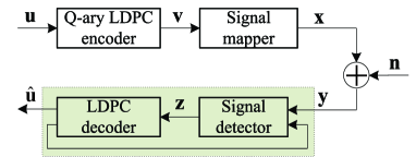
Figure 1: A nonbinary LDPC-coded modulation system

II-B LDPC Codes over GF($q$)

A $q$-ary LDPC code $\mathcal{C}$ of length $N$ over GF($q$) is given by the null space of a sparse $M\times N$ parity-check matrix $\mathbf{H}=[h_{i,j}]$ over GF($q$), where $M$ is the number of check equations and $M=N-K$ if $\mathbf{H}$ is full rank. Let $\mathbf{v}=(v_{0},v_{1},...,v_{N-1})$ be a codeword in $\mathcal{C}$. Then the parity-check constraints can be expressed as $\mathbf{vH}^{T}=\mathbf{0}$, or

$$\sum_{j=0}^{N-1}\ h_{i,j}v_{j}=0,~{}~{}i=0,1,...M-1,$$ (3)

where the operations of multiplication and addition are all defined over GF($q$). If the matrix $\mathbf{H}$ has constant row weight $d_{c}$ and constant column weight $d_{v}$, then the corresponding code is called a $(d_{v},d_{c})$-regular $q$-ary LDPC code.

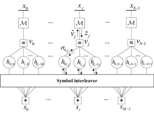
Figure 2: Forney-style factor graph of the nonbinary LDPC-coded system

Similar to its binary counterpart, a $q$-ary LDPC code can also be described using a Forney-style factor graph [16], as depicted in Fig. 2, where $\mathcal{M}$ denotes the mapper/demapper. The graph has $N$ variable nodes corresponding to coded symbols, and $M$ check nodes corresponding to parity-check equations. For convenience, we define the following two index sets

$${\mathcal{N}_{v}}(j)=\{i|h_{i,j}\neq 0,~{}0\leq i<M\},$$ (4)

$${\mathcal{N}_{c}}(i)=\{j|h_{i,j}\neq 0,~{}0\leq j<N\}.$$ (5)

III Joint Detection-Decoding Algorithm for $q$-ary LDPC-Coded Systems

In this section, we will develop an iterative joint detection-decoding algorithm for the LDPC-coded modulation system shown in Fig. 1. The whole algorithm is a hard-decision based message-passing algorithm (MPA) operating on the factor graph. Assume that a $(d_{v},d_{c})$-regular $q$-ary LDPC code is used.

III-A Signal Detection and Message-Passing Based on Hard Information

Let $\hat{\mathbf{x}}=(\hat{x}_{0},\hat{x}_{1},...,\hat{x}_{N-1})$ with $\hat{x}_{j}\in\mathcal{X}$ denote the estimate of $\mathbf{x}$ made by the signal detector based on the received vector $\mathbf{y}$. Assume that all the constellation points in $\mathcal{X}$ are used equal likely. Then with the maximum likelihood decision rule, the detected signal $\hat{\mathbf{x}}$ is given by

$$\hat{x}_{j}=\mathrm{argmin}_{x\in\mathcal{X}}\|y_{j}-x\|,~{}~{}j=0,1,...,N-1,$$ (6)

where $\|\cdot\|$ denotes the Euclidean ($l_{2}$) norm. The input of the decoder $\mathbf{z}$ is simply the demapping output of $\hat{\mathbf{x}}$, i.e.,

$$z_{j}=\mathcal{M}^{-1}(\hat{x}_{j})\in\mathrm{GF}(q),~{}~{}j=0,1,...,N-1.$$ (7)

The vector $\mathbf{z}$ is a codeword if and only if its $M$-tuple syndrome $\mathbf{s}=(s_{0},s_{1},...,s_{M-1})$ equals $\mathbf{0}$, i.e.,

$$\ \mathbf{s}\equiv\mathbf{z}\mathbf{H}^{T}=\mathbf{0}.$$ (8)

For $0\leq i<M$, the component $s_{i}$ of $\mathbf{s}$ is given by

$$s_{i}=\sum_{j\in{\mathcal{N}_{c}}(i)}\ h_{i,j}z_{j},$$ (9)

which is called a check-sum of received symbols. A received symbol $z_{j}$ is said to be checked by $s_{i}$ if $h_{i,j}\in\mathrm{GF}(q)$$\setminus\{0\}$. From (9) with $s_{i}=0$, the estimate of $v_{j}$ given by other variable nodes participating in the check-sum $s_{i}$ can be expressed as

$$\sigma_{i,j}=-h_{i,j}^{-1}(\sum_{j^{\prime}\in{\mathcal{N}_{c}}(i)\setminus j}\ {h_{i,j^{\prime}}}z_{j^{\prime}}).$$ (10)

This is the update rule for check-to-variable node message. Since the column weight of $\mathbf{H}$ is $d_{v}$, every symbol $v_{j}$ can receive $d_{v}$ estimates along the set of edges $\{(i,j)|i\in{\mathcal{N}_{v}}(j)\}$, as depicted in Fig. 2. As can be seen from (9) and (10) , only hard information propagates between variable and check nodes, i.e., the variable nodes send their hard-decision decoded symbols to the check nodes, and the check nodes simply compute the syndromes and send estimates back to their adjacent variable nodes. The estimate $\sigma_{i,j}$ for $v_{j}$ can be considered as the extrinsic information [15].

III-B Iterative Detection-Decoding

We now proceed to consider the update rule for variable nodes. Refer to Fig. 2. Assume that a variable node has received the extrinsic information from adjacent check nodes. Different from general message-passing algorithms, we will use this information to update the received samples to improve the reliability measure of received signal. To do this, an iterative process is performed between variable nodes and signal detector. For simplicity, the proposed iterative joint detection-decoding algorithm will be referred to as IJDD hereafter.

In the following, we first introduce some notations used for the IJDD algorithm. Let $k_{max}$ be the maximum number of iterations to be performed. For $0\leq k<k_{max}$, let:

• $\mathbf{y}^{(k)}=(y_{0}^{(k)},y_{1}^{(k)},...,y_{N-1}^{(k)})$ be the input vector to the signal detector in the $k$th iteration; $\hat{\mathbf{x}}^{(k)}$ and $\mathbf{z}^{(k)}$ be the corresponding detected signal vector and the output decision vector.

• $\mathbf{s}^{(k)}=(s_{0}^{(k)},s_{1}^{(k)},...,s_{M-1}^{(k)})$ be the syndrome of $\mathbf{z}^{(k)}$.

• $\sigma_{i,j}^{(k)}$ be the extrinsic information for $v_{j}$ given by the $i$th check-sum involving $v_{j}$ in the $k$th iteration.

• $\mathcal{D}(y_{j}^{(k)},r)$ denote a valid search sphere of radius $r$ centered at $y_{j}^{(k)}$.

• ${\vec{\mathbf{L}}_{j}}^{(k)}(\mathbf{p},\mathbf{q})=\mathbf{q}-\mathbf{p}$ be a correction vector directed from the point $\mathbf{p}$ to the point $\mathbf{q}$. For brevity, we will use ${\vec{\mathbf{L}}_{j}}^{(k)}$ for ${\vec{\mathbf{L}}_{j}}^{(k)}(\mathbf{p},\mathbf{q})$.

• $f_{j}^{(k)}(a)$, $a\in\mathrm{GF}(q)$ denote the number of occurrences of the element $a$ in $\{\sigma_{i,j}^{(k)}\}_{i\in\mathcal{N}_{v}(j)}$.

Clearly, $0\leq f_{j}^{(k)}(a)\leq d_{v}$ and $\sum_{a\in{\mathrm{GF}(q)}}f_{j}^{(k)}(a)=d_{v}$. $f_{j}^{(k)}(a)$ indicates a reliability measure for decoding $z_{j}$ into the symbol $a$. Let

$$a_{max}=\arg\max_{a\in\mathrm{GF}(q)}\{f_{j}^{(k)}(a)\},$$ (11)

and

$$\Delta f_{j}^{(k)}=f_{j}^{(k)}(a_{max})-\max_{a\in\mathrm{GF}(q)\setminus\{a_{max}\}}\{f_{j}^{(k)}(a)\},$$

where $a_{max}$ is the element in GF($q$) that has the highest reliability for $v_{j}$, and $\Delta f_{j}^{(k)}$ represents the difference in number of votes between the two highest-voted candidates for $v_{j}$ in the $k$th iteration. With the plurality voting rule, we choose

$$\hat{v}_{j}^{(k)}=a_{max}.$$

With the above discussions, the message update rule for variable nodes can be formulated as follows.

Message Update Rule for Variable Nodes: Make estimation on $\hat{v}_{j}^{(k)}$ using (11) based on ${\{\sigma_{i,j}^{(k)}\}}_{i\in{\mathcal{N}_{v}(j)}}$, $j=0,1,...,N-1$, and evaluate $f_{j}^{(k)}(a_{max})$ and $\Delta f_{j}^{(k)}$. Then the variable nodes send the triples $(\hat{v}_{j}^{(k)},\Delta f_{j}^{(k)},f_{j}^{(k)}(a_{max}))$, $0\leq j\leq N-1$, to detector, where the following operations are performed on $y_{j}^{(k)}$:

$$y_{j}^{(k+1)}=y_{j}^{(k)}+\xi_{j}^{(k)}{\vec{\mathbf{L}}_{j}^{(k)}},$$ (12)

Here ${\vec{\mathbf{L}}_{j}^{(k)}}$ and $\xi_{j}^{(k)}$ are given based on $\hat{x}_{j}^{(k)}$ and $(\hat{v}_{j}^{(k)},\Delta f_{j}^{(k)},f_{j}^{(k)}(a_{max}))$, $0\leq j\leq N-1$, which can be described as follows.

• If $\mathcal{M}(\hat{v}_{j}^{(k)})\in\mathcal{D}(y_{j}^{(k)},r)$, then

  $$\vec{\mathbf{L}}_{j}^{(k)}=\left\{\begin{array}[]{ll}\hat{x}_{j}^{(k)}-y_{j}^{(k)},&\mbox{{ if }$\mathcal{M}(\hat{v}_{j}^{(k)})=\hat{x}_{j}^{(k)}$}\\ \mathcal{M}(\hat{v}_{j}^{(k)})-\hat{x}_{j}^{(k)},&\mbox{{ if }$\mathcal{M}(\hat{v}_{j}^{(k)})\neq\hat{x}_{j}^{(k)}$}\end{array}\right.$$ (13)

  and

  $$\xi_{j}^{(k)}=\left\{\begin{array}[]{ll}f_{j}^{(k)}(a_{max})/{d_{v}},&\mbox{{ if }$\Delta f_{j}^{(k)}\geq T$}\\ \Delta f_{j}^{(k)}/{d_{v}},&\mbox{{ if }$\Delta f_{j}^{(k)}<T$}\end{array}\right.$$ (14)

• Otherwise set ${\vec{\mathbf{L}}_{j}^{(k)}}=\mathbf{0}$ and $\xi_{j}^{(k)}=0$.

Note that $\mathcal{D}(y_{j}^{(k)},r)$ specifies a region where $x_{j}$ is located most likely. Only $\mathcal{M}(\hat{v}_{j}^{(k)})$ within this region are used to update $y_{j}^{(k)}$. In this paper we set $r$ to be 1.415$d_{min}$ and $T$ to be 3, where $d_{min}$ is the minimum Euclidean distance among constellation points. Moreover, the case of $\mathcal{M}(\hat{v}_{j}^{(k)})$=$\hat{x}_{j}^{(k)}$ in (13) indicates that, $y_{j}^{(k)}$ may be decoded into $\hat{x}_{j}^{(k)}$ with high confidence. In other words, $y_{j}^{(k)}$ is considered as the noisy version of $\hat{x}_{j}^{(k)}$. However, instead of instantly setting $y_{j}^{(k)}$ to be $\hat{x}_{j}^{(k)}$, cautious shift is operated on $y_{j}^{(k)}$ towards $\hat{x}_{j}^{(k)}$. While in the case of $\mathcal{M}(\hat{v}_{j}^{(k)})\neq\hat{x}_{j}^{(k)}$, the received signal will be shifted towards the decision boundary of the two candidates, achieving a trade-off between the two choices. Here the decision boundary of $\mathcal{M}(\hat{v}_{j}^{(k)})$ and $\hat{x}_{j}^{(k)}$ is the bisector perpendicular to $\vec{\mathbf{L}}_{j}^{(k)}=\mathcal{M}(\hat{v}_{j}^{(k)})-\hat{x}_{j}^{(k)}$.

Then using ${\vec{\mathbf{L}}_{j}^{(k)}}$ and $\xi_{j}^{(k)}$, the detector updates currently input vector according to (12). Based on $y_{j}^{(k+1)}$, new hard-decision is made, and the results are delivered to the variable nodes as the updated message passed from detector to the decoder. The whole working process of the IJDD algorithm is shown in Fig. 3.

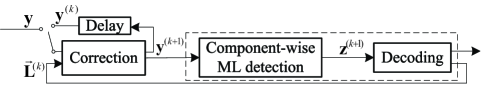
Figure 3: Iterative joint detection-decoder.

In summary, the IJDD algorithm can be formulated as follows.

 

IJDD Algorithm

 

• Initialization.
  Set $k=0$, and ${\mathbf{y}}^{(0)}=\mathbf{y}$.

• Repeat the following while $k<k_{max}$

  1. Signal detection:
     - For $j=0,1,...,N-1$, make ML decisions based on $y_{j}^{(k)}$, yielding $\hat{x}_{j}^{(k)}$ and $z_{j}^{(k)}$ as in (6) and (7).
     - Pass the message ${\mathbf{z}}^{(k)}$ to LDPC decoder.

  2. Compute syndrome and do check-node update:
     - Compute syndrome vector $\mathbf{s}^{(k)}=\mathbf{z}^{(k)}\mathbf{H}^{T}$.
     - If $\mathbf{s}^{(k)}=\mathbf{0}$, then terminate iteration and output $\hat{\mathbf{v}}^{(k)}=\mathbf{z}^{(k)}$ as the decoded codeword;
     - else for $i=0$ to $M-1$ and $j=0$ to $N-1$,
     compute check-to-variable messages $\sigma_{i,j}^{(k)}$ as in (10).

  3. Variable-node update and correction:
     For $j=0$ to $N-1$,
     - evaluate $(\hat{v}_{j}^{(k)},\Delta f_{j}^{(k)},f_{j}^{(k)}(a_{max}))$ based on $\{\sigma_{i,j}^{(k)}\}$ at variable nodes;
     - send the message triples $(\hat{v}_{j}^{(k)},\Delta f_{j}^{(k)},f_{j}^{(k)}(a_{max}))$ to detector and perform signal corrections as done in Section III-B.

  4. $k=k+1$, entering next iteration.

• If $k=k_{max}$, declare a decoding failure.

 

It is worth mentioning that in the IJDD algorithm differs from QSPA/FFT-QSPA in two aspects: 1) In the IJDD algorithm, only simple operations such as additions, comparisons, look-up tables, negligible amount of real operations and finite field operations are required; 2) The iterative process based on hard information is performed among detector/demapper, variable nodes and check nodes, while in the QSPA/FFT-QSPA, soft information propagates only between variable and check nodes.

From the above, it can be seen that the IJDD algorithm is easy to implement, and can achieve high speed. However, like existing reliability-based decoding algorithms, to ensure the reliability of majority voting, the column weights of $\mathbf{H}$ have to be relatively large. It seems not easy for randomly constructed $q$-ary LDPC codes to fulfill this requirement, thus application of IJDD algorithm is restricted to $q$-ary LDPC codes constructed based on finite fields [10] or finite geometry [11].

IV Simulation Results

In this section, two examples of $q$-ary LDPC codes are provided to demonstrate the effectiveness of the proposed IJDD algorithm.

Example 1: Consider a 16-ary (255, 175) regular LDPC code constructed based on finite fields. The factor graph of this code has 255 variable nodes and 255 check nodes (including 175 redundant check equations). Both the row and column weights are 16. With the use of 16-QAM signaling over the AWGN channel, scatter plots for signal vectors before and after decoding using IJDD with 10 iterations at $E_{b}/N_{0}=8.0$ dB are shown in Fig. 4(a) and Fig. 4(b), respectively. Clearly, the scatter plot in Fig. 4(b) corresponds to an ideal signal constellation, i.e., all received samples have been shifted to the probable originally transmitted constellation points.

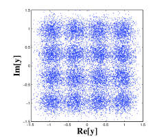
(a) Received signal space

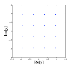
(b) Corrected signal space

Figure 4: Scatter plot of signal space before and after decoding with 10 iterations

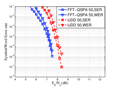
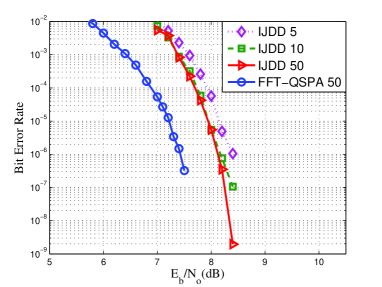
Figure 5: Error performance of the 16-ary (255,175) LDPC code decoded with the FFT-QSPA and the IJDD algorithm (16-QAM)

Figure 6: Rate of decoding convergence of the IJDD algorithm for decoding the 16-ary (255,175) LDPC code (16-QAM)

Shown in Fig. 6 are the symbol and word error performances of this coded system decoded using the IJDD algorithm and FFT-QSPA with 50 iterations. It is seen that at a SER of $10^{-6}$, the IJDD algorithm performs only 0.67dB away from the FFT-QSPA. Similar observation can be made for WER.

To illustrate the rate of decoding convergence of the IJDD algorithm, simulations were also carried out for $k_{max}=10$ and $k_{max}=5$, respectively, with results shown in Fig. 6. It is seen that with 10 and 50 iterations, the BER curves of the IJDD algorithm nearly overlap each other. Even with 5 iterations, the loss of performance is only 0.35 dB compared to IJDD with 50 iterations.

Example 2: Consider a 32-ary (1023, 781) regular LDPC code constructed based on finite fields. The row redundancy is 781 and both the row and column weights are 32. The performance of this code incorporated with 32-QAM modulation over the AWGN channel is illustrated in Fig. 7, where the codewords were obtained by encoding the randomly generated source data. Surprisingly, the IJDD algorithm outperforms the FFT-QSPA by 1.0 dB at a BER of $10^{-5}$. This result may be caused by large column weights and large row redundancy of the code, which can offer high reliability for IJDD. In addition, the large column weights and large row redundancy of the code may make the FFT-QSPA algorithm not suitable for decoding it.

V Conclusions

In this paper, we propose an iterative joint detection-decoding algorithm for $q$-ary LDPC-coded systems, which can be characterized as a hard-decision based message-passing algorithm and so has low computational complexity. For $q$-ary LDPC codes with large row redundancy and column weights, the proposed algorithm can offer good performance or even outperforms the FFT-QSPA with a lower computational complexity. Furthermore, the fast rate of decoding convergence of our proposed algorithm makes it particularly attractive, thus offering an attractive candidate for practical applications of $q$-ary LDPC codes. Although only regular LDPC codes are considered here, the proposed algorithm can be extended directly to decode irregular $q$-ary LDPC codes.

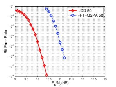
Figure 7: Error performance of the 32-ary (1023,781) LDPC code decoded with the FFT-QSPA and the IJDD algorithm (32-QAM)

References

- [1] R. G. Gallager, Low-Density Parity-check codes. Cambridge, MA: MIT Press, 1963.
- [2] M. C. Davey and D. J. C. MacKay, “Low density parity check codes over GF(),” IEEE Commun. Lett., vol. 2, no. 6, pp. 165-167, June 1998.
- [3] X.-Y. Hu and E. Eleftheriou, “Binary representation of cycle Tanner-graph GF() codes,“ in Proc. IEEE Int. Conf. Commun., Paris, France, Jun. 2004, pp. 528-532.
- [4] D. J. C. MacKay and M. C. Davey, “Evaluation of gallager codes for short block length and high rate application,” in Proc. IMA International Conference on Mathematic and its Applications: Codes, Systems and Graphincal Models, pp. 113-130, Springer-Verlag, New York, 2000.
- [5] D. Declercq and M. Fossorier, “Decoding algorithms for nonbinary LDPC codes over GF(),“ IEEE Trans. Commun., vol. 55, no. 4, pp. 633-643, Apr. 2007.
- [6] S. Song, L. Zeng, S. Lin, and K. Abdel-Ghaffar, “Algebraic constructions of nonbinary quasi-cyclic LDPC codes,“ in Proc. IEEE Int. Symp. Inform. Theory, Seattle, WA, Jul. 2006, pp. 83-87.
- [7] V. Rathi, R. Urbanke, “Density evolution, thresholds and the stability condition for non-binary LDPC codes,“ IEE Proc. Commun., vol. 152, no. 6, pp. 1069-1074, Dec. 2005.
- [8] A. Bennatan and D. Burshtein, “Design and analysis of nonbinary LDPC codes for arbitrary discrete-memoryless channels,“ IEEE Trans. Inform. Theory, vol. 52, no. 2, pp. 549-583, Feb. 2006.
- [9] G. Li, I. J. Fair, and W. A. Krzymien, “Density Evolution for Nonbinary LDPC Codes Under Gaussian Approximation,“ IEEE Trans. Inform. Theory, vol. 55, no. 3, Mar. 2009.
- [10] L. Zeng, L. Lan, Y. Tai, S. Song, S. Lin, and K. Abdel-Ghaffar, “Constructions of nonbinary quasi-cyclic LDPC codes: a finite field approach,” IEEE Trans. Commun., vol. 56, no. 4, pp. 545-554, Apr. 2008.
- [11] L. Zeng, L. Lan, Y. Tai, S. Song, S. Lin, and K. Abdel-Ghaffar, “Constructions of nonbinary quasi-cyclic LDPC codes: a finite geometry approach,” IEEE Trans. Commun., vol. 56, no. 3, pp. 378-387, Mar. 2008.
- [12] S. Lin and D. J. Costello, Jr., Error Control Coding: Fundamentals and Applications, 2nd ed. Upper Saddle River, NJ: Prentice-Hall, 2004.
- [13] N. Mobini, A. H. Banihashemi and H. Hemati, “A differential binary message-passing LDPC decoder,“ IEEE Trans. Commun., vol. 57, no. 9, pp. 2518-2523, Sep. 2009.
- [14] A. Nouh and A. H. Banihashemi, “Bootstrap decoding of low-density parity-check codes,“ IEEE Commun. Lett., vol. 6, no. 9, pp. 391-393, Sep. 2002.
- [15] Q. Huang, J. Y. Kang, L. Zhang, S. Lin and K. Abdel-Ghaffar, “Two reliability-based iterative majority-logic decoding algorithms for LDPC codes,“ IEEE Trans. Commun., vol. 57, no. 12, Dec. 2009.
- [16] G. D. Forney Jr., “Codes on graphs: Normal realizations,” IEEE Trans. Inform. Theory, vol. 47, pp. 520-548, Feb. 2001.