Mathematical Modeling of Competition in Sponsored Search Market

Abstract

Sponsored search mechanisms have drawn much attention from both academic community and industry in recent years since the seminal papers of [13] and [14]. However, most of the existing literature concentrates on the mechanism design and analysis within the scope of only one search engine in the market. In this paper we propose a mathematical framework for modeling the interaction of publishers, advertisers and end users in a competitive market. We first consider the monopoly market model and provide optimal solutions for both ex ante and ex post cases, which represents the long-term and short-term revenues of search engines respectively. We then analyze the strategic behaviors of end users and advertisers under duopoly and prove the existence of equilibrium for both search engines to co-exist from ex-post perspective. To show the more general ex ante results, we carry out extensive simulations under different parameter settings. Our analysis and observation in this work can provide useful insight in regulating the sponsored search market and protecting the interests of advertisers and end users.

1 Introduction

Internet advertising has become a main source of revenue for primary search engines nowadays. According to the newly-released report by Interactive Advertising Bureau and PricewaterhouseCoopers [1], Internet advertising in the United States reached $22.7 billion in total revenue for the full year of 2009, where sponsored search revenue accounted for 47 percent of the total revenue.

A typical Internet search market consists of three parties: publishers (i.e., search engines), advertisers and end users. In the current age of information explosion, more and more people rely on search engines to pin down their favored products or services. Whenever a query is submitted to the engines by end users, their intents or interests can be potentially captured by the engines through the inputted keywords. These intents of search users can then be sold by search engines to companies who are interested in targeting their products to these users. Nowadays, major search engine operators like Google, Yahoo! and Microsoft display advertisements in the form of sponsored links, which appears alongside the algorithmic links (also known as organic links) in the search results pages. For each keyword, there are usually more than one available advertising slot in the search engine results page. How to effectively allocate these slots and charge the advertisers have been studied and discussed extensively in recent years among people in both academia and industry. Take Google’s AdWords program for example. In this advertising program, advertisers could choose multiple keywords they are interested in, and for each keyword indicate the maximal willingness to pay for each click and the budget to spend over a period of time. Whenever a user clicks on the sponsored link and is re-directed to the advertisers’ site, certain payment is charged by the program until the advertisers’ budget is used up.

Most of the existing works focus on the interaction of the three parties within the scope of only one search engine’s advertising system, and these results and suggestions from researchers did greatly improve the efficiency of mechanism held in major search engine companies. For example, the transition from generalized first price auction to generalized second price auction, from payment per impression to payment per click, from bid-based ranking to quality-based ranking and so on [2, 6]. However, considering there is usually more than one company providing search service in the market, one natural question would be how the market would evolve when there exists competition between multiple search engines. In particular, will all users and advertisers gradually concentrate to one leading engine or will the “inferior” engines still earn enough profits to survive when competing with the leading one? What would be the consequences if one search engine monopolizes the market? Should governments take anti-trust action against potential cooperation among major search engines? These concerns arise from the current situation of high levels of concentration in search engine market: Google is widely considered to possess the leading technology and obtain the largest market shares in most countries and regions, followed by Yahoo! and Microsoft Bing.

This paper aims to formulate a reasonable model to study the competition between two search engine operators and help to address some of the intriguing questions mentioned above. We will consider a three-stage dynamic game model. In stage I, the two operators’ services determine how the market of end users is split. In stage II, the two operators simultaneously determine their prices to advertisers. In stage III, the advertisers choose the operator in which they can obtain highest utility based on the announced prices in stage II. Each operator wants to maximize its revenue subject to the competition for advertisers from the other operator.

The key contributions of the paper are:

• To the best of our knowledge, this paper is among the first to model the comprehensive interaction of heterogenous publishers, advertisers and users in a competitive environment. We elaborate the whole process of search engine competition in attracting both users and advertisers. The technical details applied in practical advertising systems, such as the values and budgets of advertisers, are taken into consideration explicitly in our formulation.

• We prove the existence of Nash Equilibrium prices when allowing advertisers participate in both advertising systems simultaneously. Moreover, we show the comparative results between the equilibrium prices and monopoly price when only one search engine exists in the market.

• We propose two distinct points of view, i.e., the ex ante view and the ex post view, to inspect the long-term and short-term revenues of search engines respectively. Furthermore, for the ex post case, we present the detailed algorithm for calculating the exact allocation results for advertisers. For the ex ante case, we can carry out the simulations to illustrate the comparative results of expected revenues and social welfare under competition and monopoly respectively.

The paper is organized as follows. Section 2 presents the related work. Section 3 formulates the monopoly model and provides solutions for both the ex ante and ex post cases. Based on the monopoly formulation, we analyze the strategic behaviors of end users and advertisers under duopoly and find the Nash Equilibrium prices of both search engines in Section 4. In Section 5 we compare the results under competition and monopoly via simulation and reveal various factors that affect the revenues and social welfare. We conclude in Section 6 and outline some future research directions.

2 Related Work

There are mainly two lines of research work in the sponsored search area. The mainstream of literature focuses on the interaction between advertisers and search engines and aims to understand and devise viable mechanism for the Internet advertising market. There is significant work on the auction mechanism held by major search engines, starting from two seminal works of [13] and [14] which independently investigated the “generalized second-price” (GSP) auction prevailing in major search engines such as Google and Yahoo!. In [20] the authors compared the “direct ranking” method by Overture with the “revenue ranking” method by Google and proposed a truthful mechanism named as “laddered auction”. Considering the non-strategyproofness property of GSP mechanism, [21] analyzed one prevalent strategy of advertisers called “vindictive bidding” in real-world keyword auction. [26] and [27] relaxed the basic assumption of separable click-through rate in [20] and modeled the externality effect among advertisements which appeared in the same search page simultaneously. [28] proposed a new valuation model to absorb the adverse effect of the competing advertisements on the advertiser’s value per click. There is also an abundance of works on proposing more expressive but still scalable mechanism for sponsored search such as [24, 25, 23, 29, 22]. In particular, in [29] the advertisers were allowed to submit a two-dimensional bid $(b,b^{\prime})$ where $b$ was the bid for exclusive display and $b^{\prime}$ for sharing slots with other advertisements. In [22] the authors proposed a truthful hybrid auctions where advertisers can make a per-impression as well as per-click bid and showed that it can generate higher revenue for search engine compared with the pure per-click scheme.

It’s worth pointing out that a few works considered the practical situation where similar keyword auctions are held simultaneously by multiple search engines. For example, in [15] the authors investigated the revenue properties of two search engines with different click-through rates which competed for the same set of advertisers. The study in [16] considered competition between two search engines which differs in their ranking rules: one applied the direct ranking method we mentioned above, and the other applied the revenue ranking method. We assert that this assumption of search engine difference is unrealistic since major engines tend to use the same policy which proves to work efficiently in practice and it is unlikely that certain engine would switch back to the obsolete rules. The Nash equilibrium solution in the former paper of [15] is also not so practical since it requires advertisers to adopt certain randomized strategy. It’s very difficult for individual advertisers to implement such complex strategies which would incur unnecessary maintenance cost.

The other line of work is developed mainly by economists to address the broad issues of search engine competition from social welfare perspective. [4] introduced a quality choice game model where end users choose the search engine with highest quality of search results, and showed that no Nash equilibrium exists in this game. Based on this proposition, the author argues that the search engine market would evolve towards monopoly in the absence of necessary regulatory interventions. [5] proposed a duopoly model which has some similarity to our formulation, however, as many of the technical details of the practical advertising system are ignored, it is doubtful whether this can serve as an accurate model to predict the outcome of search engine market. Similarly, [4] faces the same problem that the vague description of participants’ utility may not be strong enough to support the predictive conclusions in the paper.

These two lines of important work have little intersections so far: the mainstream of work concentrates on the technical progress in designing “better” advertising system, and the other line usually involves less technical details (like the budgets of advertisers in practical advertising system) and targets the macro-effect of competitive market. In view of this, we believe that a comprehensive study of the current search engine ecosystem in a competitive way is vital for addressing many of the unresolved issues in this thriving market. Our work manages to narrow the gap between these two directions of research and makes some initial progress in this direction. This observation helps differentiate our work from most of the existing literature.

3 The Monopoly Market Model

In this section we consider the monopoly market first, which serves as a starting point for analyzing the more general competition market. Suppose there is only one search engine in the market servicing a fixed set of end users and providing advertising opportunity for a set of advertisers denoted by $\mathcal{I}$ ($|\mathcal{I}|=m$). Assuming all users are homogeneous and each of them tends to generate the same number of impressions (or clicks) for a particular keyword (query). Since we assumes that the search engine owns a fixed number of users, it would be able to supply a fixed number of attentions (in the form of impressions or clicks) for advertisers. For a given interval, let the supply of attentions be $S$. Each advertiser $i\in\mathcal{I}$ has two private parameters: value $v_{i}$ denoting $i$’s maximal willingness to pay for each attention and budget $B_{i}$ in a given time interval (could be daily, weekly, monthly budget and so on). The search engine needs to determine the optimal price per attention to maximize its revenue:

$$R=p\cdot\min(S,D(p))=\min(p\cdot S,pD(p))$$

where $D(p)$ is the demand function over price $p$.

In the following analysis we consider this revenue maximization problem in two different perspectives: the ex ante perspective where the search engine only has an rough estimation to the parameters of participating advertisers, and the ex post perspective where the engine just needs to make decision based on the submitted parameters of advertisers. Although in practice, the advertising systems do determine the prices only after advertisers have submitted their values and budgets, we assert that the ex ante view of revenue to be a natural fit for the search engine’s objective. This is because typically the interaction between search engine and advertisers is not one-shot and would usually last for many rounds. Advertisers can actually adjust their submitted parameters at any time to achieve better payoff. Thus the ex ante result could provide valuable prediction of the long-term revenue for the search engine, rather than the short-term profit from one particular instance of the ex post case.

3.1 Ex ante case

Assuming the search engine can have a rough estimation of the distribution of advertisers’ values and budgets. For simplicity, we only consider the scenario when the parameters are independent and identically-distributed random variables. To be specific, suppose values are drawn independently from distribution with density function $f(v)$ and CDF $F(v)$ over the range of $[\underline{v},\overline{v}]$, and budgets are drawn independently from distribution with density function $g(B)$ and CDF $G(B)$.

After search engine announce the uniform price $p$, advertiser $i$ would make the deal if only the value $v_{i}$ is larger than $p$. The quantity advertiser $i$ could purchase is constrained by the budget $B_{i}$.

Therefore the expected aggregate demand under price $p$ from all advertisers would be:

$$D(p)=\sum_{i\in\mathcal{I}}\frac{E(B_{i})}{p}\cdot\mbox{Prob}\{v_{i}>p\}=m\cdot\frac{E(B)}{p}[1-F(p)]$$

Rewrite it as:

$$p\cdot D(p)=m\cdot{E(B)}\cdot[1-F(p)]$$ (1)

which is a non-increasing function over $p$.

We can use figure 1 to illustrate the revenue of search engine over price $p$.

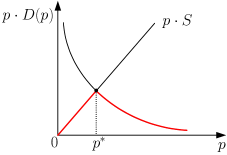
Figure 1: Search Engine Revenue Over Prices (Ex Ante)

Proposition 1.

The revenue $R$ is maximized when $S=D(p)$, i.e., when the demand equals the supply.

Proposition 1 can be proved by contradiction. If supply exceeds demand under the current price, the search engine will cut down the price to achieve higher revenue (since $R=p\cdot D(p)$ is non-increasing over price $p$); if demand exceeds supply, the search engine can raise the price and reach a higher revenue (since $R=p\cdot S$ is monotonically increasing over price $p$).

Example 1.

Assuming $v_{i}$ is drawn from uniform distribution with positive support on the interval $[\underline{v},\overline{v}]$, where $0\leq\underline{v}<\overline{v}$ and $\Delta v=\overline{v}-\underline{v}$. Then $1-F(p)=\frac{\overline{v}-p}{\Delta v}$. From $S=D(p)$ we have:

$$p^{*}=\frac{m\cdot E(B)\cdot\overline{v}}{m\cdot E(B)+S\cdot\Delta v}$$

The intuition is that the more demand (larger $m$) there is, the higher market clearing price would be; and the more supply (larger $S$) there is, the lower market clearing price is.

3.2 Ex post case

In practical search engine advertising system, advertisers need to submit their values and budgets to the advertising system. The search engine therefore could determine the optimal price based on the ex post variables.

Reorder the index of advertisers such that $v_{j}\leq v_{j+1},j=1,\ldots,m-1$. Then the aggregate demand can be written as:

$$D(p)=\sum_{i\in\mathcal{I}^{+}(p)}\frac{B_{i}}{p}$$

where we define the set:

$${\mathcal{I}^{+}(p)}\triangleq\{i\in\mathcal{I}:v_{i}>p\}$$

Thus $p\cdot D(p)=\sum_{i\in\mathcal{I}^{+}(p)}B_{i}$ is a non-increasing function over $p$ since ${\mathcal{I}^{+}(p)}$ shrinks as price $p$ increases. By letting demand equal to supply, we have

$${p}(\mathcal{I})=\frac{\sum_{i\in\mathcal{I}^{+}({p})}B_{i}}{S}$$

Notice that the term of price appears in both sides of the equation. Thus in general we cannot derive the closed-form solution for optimal price. Since $pD(p)$ is piece-wise constant and (weakly) decreasing over $p$, we can illustrate the search engine revenue through examples in figure 2. Here we assume there are four advertisers ordered such that $v_{1}\leq v_{2}\leq v_{3}\leq v_{4}$ and initially when the price is zero, ${\mathcal{I}^{+}(p)}=\mathcal{I}=\{1,2,3,4\}$. As the price exceeds $v_{1}$, advertiser $1$ would have no incentive to stay and ${\mathcal{I}^{+}(p)}$ becomes $\{2,3,4\}$. The crossing point of demand and supply shows that the optimal price $p^{*}$ is located in $[v_{1},v_{2}]$. To be more exact, $p^{*}(\mathcal{I})=(B_{2}+B_{3}+B_{4})/S$. In figure 2b we also show the other case when there is one advertiser who is indifferent between participating and quitting the ad campaign since the optimal price is equal to its value. In typical search engine systems like Google AdWords, after advertisers input their maximal willingness to pay (i.e., their values) and budgets, the ad system would automatically allocate attentions to advertisers as long as the current price doesn’t exceed their values and the budgets have not been exhausted yet. Thus here for ease of expression we can assume that the indifferent advertiser would continue participating in the ad campaign under the budget constraint. For example, as shown in figure 2b, the optimal price is equal to $v_{2}$ (satisfying $B_{3}+B_{4}<v_{2}S<B_{2}+B_{3}+B_{4}$), advertiser 2 would consume the remaining supply of $S-\frac{B_{3}+B_{4}}{v_{2}}$ and only spent $v_{2}S-B_{3}-B_{4}$ which is less than its budget $B_{2}$.

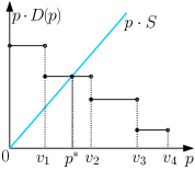
(a) Determined Advertisers

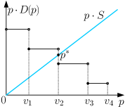
(b) Undetermined Advertiser

Figure 2: Search Engine Revenue Over Prices (Ex Post)

We can now show a polynomial step algorithm for search engine to compute the optimal price. By inputting the parameters of advertisers (assuming the indexes of advertisers are re-ordered such that $v_{i}\leq v_{i+1}$, $i\in\{1,\ldots,m-1\}$), algorithm 1 would return the value of optimal price. The time complexity of the algorithm is $O(m^{2})$ where $m$ is the number of advertisers.

Algorithm 1 Calculate Optimal Price $p^{*}(\mathcal{I})$

0:  

1:  $v_{0}=0$;

2:  for $i=1:m$

3:        $sum=0$;

4:        for $j=i:m$

5:              $sum+=B_{j}$;

6:        end for;

7:        $p=sum/S$;

8:        if $(p\leq v_{i})$

9:              return $\max(p,v_{i-1})$;

10:        end if;

11:  end for;

12:  return $v_{m}$;

12:  

After determining the optimal price $p^{*}$, the quantity of attentions allocated to each advertiser $i$, denoted by $q_{i}$, can be easily computed. The search engine would first find the least index of advertiser whose value is larger than or equal to $p^{*}$, which is denoted by $j\in\{i\in\mathcal{I}:v_{i}\geq p^{*},v_{i-1}<p^{*}\}$ (we define $v_{0}=0$). If there are no undetermined advertisers, which implies $v_{j}>p^{*}$, the quantity allocated to advertiser $i$ would be $q_{i}=B_{i}/p^{*}$ for $i\geq j$ and $q_{i}=0$ otherwise. If undetermined advertiser does exist, which implies $v_{j}=p^{*}$, we have $q_{i}=B_{i}/p^{*}$ for $i>j$, $q_{j}=S-\sum_{i=j+1}^{m}q_{i}$, and $q_{i}=0$ for $i<j$. In both cases, the demand equals the supply, i.e., $\sum_{i\in\mathcal{I}}q_{i}=S$. This can be summarized in algorithm 2.

Algorithm 2 Calculate Allocation $q_{i}$, $i\in\mathcal{I}$

0:  

1:  $sum=0$;

2:  $p=p^{*}$;

3:  for $j=1:m$

4:        if $(v_{j}\geq p)$

5:              break;

6:        end if;

7:  end for;

8:  for $i=1:(j-1)$

9:        $q_{i}=0;$

10:  end for;

11:  for $i=(j+1):m$

12:        $q_{i}=B_{i}/p$;

13:        $sum+=q_{i}$;

14:  end for;

15:  $q_{j}=S-sum$;

15:  

The revenue of search engine is:

$$R=p^{*}\cdot S$$ (2)

The aggregate utility of advertisers is:

$$U_{A}=\sum_{i\in\mathcal{I}^{+}(p^{*})}(v_{i}-p^{*})\frac{B_{i}}{p^{*}}$$ (3)

Notice that the indifferent advertiser, if exists, would always achieve zero utility since the current price equals its value, thus we don’t need to consider it in the expression.

The social welfare of the advertising system is:

$$SW=R+U_{A}$$ (4)

Lemma 1.

The optimal price is non-decreasing over the set of participating advertisers given fixed supply $S$. That is to say, for any advertisers set $\mathcal{I}_{1}$ and $\mathcal{I}_{2}$, if $\mathcal{I}_{1}\subseteq\mathcal{I}_{2}$, we have $p^{*}(\mathcal{I}_{1})\leq p^{*}(\mathcal{I}_{2})$, where $p^{*}(\mathcal{I})$ is obtained according to algorithm 1.

Proof.

We can prove the above lemma by contradiction. For simplicity of notation, we write $p_{1}\triangleq p^{*}(\mathcal{I}_{1})$ and $p_{2}\triangleq p^{*}(\mathcal{I}_{2})$ and assume that $p_{1}>p_{2}$.

Since under optimal price, supply must be equal to demand, we have:

$$S=\sum_{i\in\mathcal{I}_{1}^{+}(p_{1})}\frac{B_{i}}{p_{1}}+\frac{\alpha B_{l}}{p_{1}}\quad\mbox{and}\quad S=\sum_{i\in\mathcal{I}_{2}^{+}(p_{2})}\frac{B_{i}}{p_{2}}+\frac{\beta B_{l^{\prime}}}{p_{2}}$$

where $\alpha\in[0,1]$, and $\alpha>0$ if and only if there exists an indifferent advertiser $l$ whose value $v_{l}$ equals $p_{1}$; Similarly, $\beta\in[0,1]$, and $\beta>0$ if and only if there exists an advertiser $l^{\prime}$ such that $v_{l^{\prime}}=p_{2}$.

For any advertiser $i\in\mathcal{I}_{1}^{+}(p_{1})$, we have $i\in\mathcal{I}_{1}\subseteq\mathcal{I}_{2}$ and $v_{i}>p_{1}>p_{2}$, thus $i\in\mathcal{I}_{2}^{+}(p_{2})$, which infers that $\mathcal{I}_{1}^{+}(p_{1})\subseteq\mathcal{I}_{2}^{+}(p_{2})$; since $v_{l}=p_{1}>p_{2}$, we also have $l\in\mathcal{I}_{2}^{+}(p_{2})$. Therefore,

$$S=\sum_{i\in\mathcal{I}_{1}^{+}(p_{1})}\frac{B_{i}}{p_{1}}+\frac{\alpha B_{l}}{p_{1}}\leq\sum_{i\in\mathcal{I}_{1}^{+}(p_{1})}\frac{B_{i}}{p_{1}}+\frac{B_{l}}{p_{1}}\leq\sum_{i\in\mathcal{I}_{2}^{+}(p_{2})}\frac{B_{i}}{p_{1}}<\sum_{i\in\mathcal{I}_{2}^{+}(p_{2})}\frac{B_{i}}{p_{2}}\leq\sum_{i\in\mathcal{I}_{2}^{+}(p_{2})}\frac{B_{i}}{p_{2}}+\frac{\beta B_{l^{\prime}}}{p_{2}}$$

Contradiction to the conclusion that supply should equal demand under optimal price $p_{2}$. ∎

Lemma 2.

The revenue of search engine is non-decreasing over the set of participating advertisers given fixed supply $S$. That is to say, for any advertisers set $\mathcal{I}_{1}$ and $\mathcal{I}_{2}$, if $\mathcal{I}_{1}\subseteq\mathcal{I}_{2}$, we have $R(\mathcal{I}_{1})\leq R(\mathcal{I}_{2})$.

Proof.

This conclusion can be deducted from lemma 1 immediately:

$$R(\mathcal{I}_{1})=p^{*}(\mathcal{I}_{1})\cdot S\leq p^{*}(\mathcal{I}_{2})\cdot S\leq R(\mathcal{I}_{2}).$$

∎

Lemma 3.

The optimal price is non-increasing over the supply given the set of participating advertisers $\mathcal{I}$. That is to say, for any supply $S_{1},S_{2}\in[0,\infty)$, if $S_{1}>S_{2}$, we have $p^{*}(S_{1})\leq p^{*}(S_{2})$.

Proof.

We prove the lemma by contradiction. For simplicity, we write $p_{1}\triangleq p^{*}(S_{1})$ and $p_{2}\triangleq p^{*}(S_{2})$ and assume that $p_{1}>p_{2}$.

Since under optimal price, supply equals demand, we get:

$$S_{1}=\sum_{i\in\mathcal{I}^{+}(p_{1})}\frac{B_{i}}{p_{1}}+\frac{\alpha B_{l}}{p_{1}}\quad\mbox{and}\quad S_{2}=\sum_{i\in\mathcal{I}^{+}(p_{2})}\frac{B_{i}}{p_{2}}+\frac{\beta B_{l^{\prime}}}{p_{2}}$$

where $\alpha\in[0,1]$, and $\alpha>0$ if and only if there exists an indifferent advertiser $l$ whose value $v_{l}$ equals $p_{1}$; Similarly, $\beta\in[0,1]$, and $\beta>0$ if and only if there exists an advertiser $l^{\prime}$ such that $v_{l^{\prime}}=p_{2}$.

For any advertiser $i\in\mathcal{I}^{+}(p_{1})$, we have $v_{i}>p_{1}>p_{2}$, thus $i\in\mathcal{I}^{+}(p_{2})$, which infers that $\mathcal{I}^{+}(p_{1})\subseteq\mathcal{I}^{+}(p_{2})$; since $v_{l}=p_{1}>p_{2}$, we also have $l\in\mathcal{I}^{+}(p_{2})$. Therefore,

$$S_{1}=\sum_{i\in\mathcal{I}^{+}(p_{1})}\frac{B_{i}}{p_{1}}+\frac{\alpha B_{l}}{p_{1}}\leq\sum_{i\in\mathcal{I}^{+}(p_{1})}\frac{B_{i}}{p_{1}}+\frac{B_{l}}{p_{1}}\leq\sum_{i\in\mathcal{I}^{+}(p_{2})}\frac{B_{i}}{p_{1}}<\sum_{i\in\mathcal{I}^{+}(p_{2})}\frac{B_{i}}{p_{2}}\leq\sum_{i\in\mathcal{I}^{+}(p_{2})}\frac{B_{i}}{p_{2}}+\frac{\beta B_{l^{\prime}}}{p_{2}}=S_{2}$$

Contradiction to our assumption of $S_{1}>S_{2}$. ∎

Lemma 4.

The revenue of search engine is non-decreasing over the supply given the set of participating advertisers $\mathcal{I}$. That is to say, for any supply $S_{1},S_{2}\in[0,\infty)$, if $S_{1}>S_{2}$, we have $R(S_{1})\geq R(S_{2})$.

Proof.

For simplicity, we write $p_{1}\triangleq p^{*}(S_{1})$ and $p_{2}\triangleq p^{*}(S_{2})$ and from lemma 3 we know that $p_{1}<p_{2}$.

Since under optimal price, supply equals demand, we get:

$$S_{1}=\sum_{i\in\mathcal{I}^{+}(p_{1})}\frac{B_{i}}{p_{1}}+\frac{\alpha B_{l}}{p_{1}}\quad\mbox{and}\quad S_{2}=\sum_{i\in\mathcal{I}^{+}(p_{2})}\frac{B_{i}}{p_{2}}+\frac{\beta B_{l^{\prime}}}{p_{2}}$$

where $\alpha\in[0,1]$, and $\alpha>0$ if and only if there exists an indifferent advertiser $l$ whose value $v_{l}$ equals $p_{1}$; Similarly, $\beta\in[0,1]$, and $\beta>0$ if and only if there exists an advertiser $l^{\prime}$ such that $v_{l^{\prime}}=p_{2}$.

For any advertiser $i\in\mathcal{I}^{+}(p_{2})$, we have $v_{i}>p_{2}>p_{1}$, thus $i\in\mathcal{I}^{+}(p_{1})$, which infers that $\mathcal{I}^{+}(p_{2})\subseteq\mathcal{I}^{+}(p_{1})$; since $v_{l^{\prime}}=p_{2}>p_{1}$, we also have $l^{\prime}\in\mathcal{I}^{+}(p_{1})$. Therefore,

$$R(S_{2})=p_{2}\cdot S_{2}=\sum_{i\in\mathcal{I}^{+}(p_{2})}B_{i}+\beta B_{l^{\prime}}\leq\sum_{i\in\mathcal{I}^{+}(p_{2})}B_{i}+B_{l^{\prime}}\leq\sum_{i\in\mathcal{I}^{+}(p_{1})}B_{i}\leq\sum_{i\in\mathcal{I}^{+}(p_{1})}B_{i}+\alpha B_{l}=R(S_{1})$$

∎

3.3 Formulated As An Optimization Problem

The revenue maximization problem confronting the monopolistic search engine could also be interpreted as an optimization problem as follows:

maximize $$p\cdot\sum_{i}q_{i}$$ (5)

subject to $$\forall i\in\mathcal{I}:p\cdot q_{i}\leq B_{i}$$ (9)

$$\forall i\in\mathcal{I}:(v_{i}-p)\cdot q_{i}\geq 0$$

$$\sum_{i}q_{i}\leq S$$

$$\forall i\in\mathcal{I}:p,q_{i}\geq 0$$

where the search engine needs to determine its optimal price $p$ and allocation of supply $q_{i}$ to each advertiser $i$ in objective function 5. Constraint (9) means that each advertiser could not spend more than its budget. Constraint (9) shows that the utility of advertiser must be non-negative, i.e., when the price $p$ exceeds the value $v_{i}$, which implies that $q_{i}$ must be zero, advertiser $i$ would just quit the ad campaign. The total supply to all advertisers is limited by $S$, which is shown in constraint (9). The last constraint states that all variables ($p$ and $q_{i}$, $i\in\mathcal{I}$) should be non-negative.

As we have shown in proposition 1 that the maximal revenue can only be obtained when supply equals demand, therefore the above formulation may be further reduced to:

maximize $$p\cdot S$$ (10)

subject to $$\forall i\in\mathcal{I}:p\cdot q_{i}\leq B_{i}$$ (14)

$$\forall i\in\mathcal{I}:(v_{i}-p)\cdot q_{i}\geq 0$$

$$\sum_{i}q_{i}=S$$

$$\forall i\in\mathcal{I}:p,q_{i}\geq 0$$

where constraint (14) becomes tight and the objective function is simplified to maximize variable $p$ only. Thus it’s easy to see that the optimal solution for $p$ is unique. Otherwise, if both $p^{*}$ and ${p^{*}}^{\prime}$ maximize the objective function, it must be $p^{*}\cdot S={p^{*}}^{\prime}\cdot S$, so $p^{*}={p^{*}}^{\prime}$. It remains to be inspected whether the optimal allocation vector of $\vec{q}\triangleq(q_{1},q_{2},\ldots,q_{m})$ for the optimization problem is unique too. We summarize our conclusions in the following proposition.

Proposition 2.

In general, for revenue maximization problem (10), the optimal price $p$ is unique, however, there may be multiple optimal solutions for allocation vector $\vec{p}$.

This can be shown by constructing a simple example as follows: there are two advertisers with $v_{1}=1,v_{2}=2$ and $B_{1}=2,B_{2}=1$, search engine’s supply is $S=2$. Assuming the optimal price $p^{*}$ is larger than $1$, $q_{1}$ must be zero since $v_{1}<p^{*}$, then $q_{2}$ must be $2$ according to constraint (14). This would lead to $p\cdot q_{2}>2$, which contradicts with the budget constraint of $B_{2}=1$. Now assuming the optimal price $p^{*}=1$, the constraints of the optimization problem would be reduced to $q_{1}+q_{2}=2$ and $q_{2}\leq 1$, thus the optimal allocation vector could be $\vec{q^{*}}=(q_{1}^{*},q_{2}^{*})=(2-q,q)$, $\forall q\in[0,1]$.

We now turn to investigate the effect of different optimal solutions to the social welfare. Since in general $R=p\cdot\sum_{i\in\mathcal{I}}q_{i}$ and $U_{A}=\sum_{i\in\mathcal{I}}(v_{i}-p)q_{i}$, from equation (4) we get $SW=\sum_{i\in\mathcal{I}}v_{i}\cdot q_{i}$, where the payments between search engine and advertiser are crossed off. If we examine the original social welfare maximization (SWM) problem under the same constraints (14)-(14), we can immediately present a trivial solution as follows: $p=0$, $q_{m}=S$, $q_{i}=0$ for $i\in\mathcal{I}\backslash\{m\}$, i.e., letting the advertiser with the highest value acquire all the supply exclusively. Now the maximal social welfare would be $SW_{max}=v_{m}\cdot S$. However, this solution is infeasible since it induces zero profit to the search engine. An alternative problem the search engine may be interested in is to maximize the social welfare while maintaining the optimal revenue it has achieved in (10). In other words, we need to pick out one among the multiple optimal allocations of (10) to maximize the social welfare. We call it as the constrained social welfare maximization (C-SWM) problem henceforth. This following theorem gives the solution to the C-SWM problem.

Theorem 1.

Among all optimal solutions to the profit maximization problem (10), algorithm 1 and 2 yield the one which maximizes the social welfare, i.e., the solution to the constrained social welfare maximization (C-SWM) problem.

Proof.

Denote the optimal price and allocation induced by algorithms as $p^{*}$ and $q_{1}^{*},\ldots,q_{m}^{*}$, and assuming there is another allocation vector $\hat{q}_{1},\ldots,\hat{q}_{m}$ satisfying the constraints (14)-(14). Assuming advertiser $j$ has the cutting-off value such that $v_{i}\geq p^{*}$ for $i\geq j$ and $v_{i}<p^{*}$ for $i<j$. Therefore from constraint (14), we must have $q_{i}^{*}=\hat{q}_{i}=0$ for all $i<j$. According to algorithm 2, $q_{i}^{*}=\frac{B_{i}}{p^{*}}$ for all $i>j$ and $q_{j}^{*}=S-\sum_{i=j+1}^{m}q_{i}$. Due to the constraint (14), for all $i>j$, it must be $\hat{q}_{i}\leq\frac{B_{i}}{p^{*}}=q_{i}^{*}$. Hence we can assume that $\hat{q}_{i}=q_{i}^{*}-\delta_{i}$, where $\delta_{i}\geq 0$ for all $i>j$. Then the social welfare under either allocation is:

$$SW_{1} = \sum_{i\in\mathcal{I}}v_{i}\cdot q_{i}^{*}$$

$$= \sum_{i=j+1}^{m}v_{i}\cdot q_{i}^{*}+v_{j}\cdot(S-\sum_{i=j+1}^{m}q_{i}^{*})$$

$$SW_{2} = \sum_{i\in\mathcal{I}}v_{i}\cdot\hat{q}_{i}$$

$$= \sum_{i=j+1}^{m}v_{i}\cdot(q_{i}^{*}-\delta_{i})+v_{j}\cdot[S-\sum_{i=j+1}^{m}(q_{i}^{*}-\delta_{i})]$$

$$= SW_{1}+\sum_{i=j+1}^{m}\delta_{i}\cdot(v_{j}-v_{i})$$

Since $\delta_{i}\geq 0$ and $v_{j}\leq v_{i}$ for $i>j$, we have $SW_{2}\leq SW_{1}$. Therefore $q_{1}^{*},\ldots,q_{m}^{*}$ maximizes the social welfare over all possible optimal allocations of (10). ∎

4 The Duopoly Market Model

In this section we switch from the monopoly model to the competitive model with more than one search engine. Considering the likely situation where there is one leading search company and one major competitor in the market (for example, Google and Yahoo! in the United States), we describe a duopoly model where one search engine has an advantage over the other. We formulate their competition as a three-stage dynamic game and solve it from the ex post perspective as follows.

4.1 Competition for End Users in Stage I

In Stage I search engines would choose different strategies for attracting end users with different tastes. The user bases they attract in this Stage would be the decisive factor for determining their supply of user attentions to advertisers in subsequent stages.

We assume that there are two horizontally and vertically differentiated search engines $\mathcal{J}=\{1,2\}$ providing search results to users and selling ad opportunity to advertisers.

Here horizontal difference means the different design of their home pages and diversity of extra services such as email, news and other applications. Different users may have different tastes and preferences and hence be attracted by different search engines.

Vertical difference means the quality of searching results. The higher the quality is, the better users and advertisers would feel. We assume that search engine 1 possesses the leading technology to match ads to search queries and can provide better service for both users and advertisers than search engine 2.

In terms of horizontal difference, the canonical Hotelling’s model of spatial competition [7] provides an appealing framework to address the equilibrium in characteristic space. The behaviors of providers could then be rationalized as the best-response strategies of players in a location game. The dynamics of the game can be described as follows: each provider chooses a location in the characteristic space which denotes the specific feature of service it provides to users. And each user is characterized by an address reflecting his individual preference of ideal features search engines should provide. Searching at engine $j\in\mathcal{J}$ involves quadratic transportation cost for a user if engine $j$ is not located in his ideal position. Users would choose search engine which provides better search results and also induces as low transportation cost as possible.

Assuming that a continuum of users are spread uniformly with unit density on the circumference of a unit circle. The address of user is denoted by $t\in[0,1)$. Without loss of generality, let search engine 1 locate at $x_{1}=0$ and search engine 2 $x_{2}\in[0,1)$, as shown in figure 3.

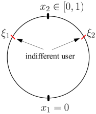
Figure 3: Users in Circular Domain

Assuming search engine 1 can provide higher quality results for users than search engine 2. Then the utility of the user searching in either engine would be as follows:

$$u_{1}(t) = \zeta_{1}q-C(t,x_{1})=q-\min\{t^{2},(1-t)^{2}\}$$ (15)

$$u_{2}(t) = \zeta_{2}q-C(t,x_{2})=\zeta q-(t-x_{2})^{2}$$ (16)

where $\zeta\in[0,1]$ denotes the comparative “disability” of search engine 2 to provide the best search result to users; $q$ is the positive payoff users perceive when certain information is returned by the search engine for a particular query; $C(t,x_{j})$ is the transportation cost incurred when there is some distance between user’s address $t$ and search engine $j$’s location $x_{j}$.

Let $u_{1}(\xi)=u_{2}(\xi)$ we can find the location of users who are indifferent between searching in two engines:

$$\xi_{1} = \frac{(1-\zeta)q+x_{2}^{2}}{2x_{2}}$$

$$\xi_{2} = \frac{1-x_{2}^{2}-(1-\zeta)q}{2(1-x_{2})}$$

Then the market share of search engine 2 is

$$n_{2}(x_{2})=\xi_{2}-\xi_{1}=\frac{1}{2}[1-\frac{(1-\zeta)q}{x_{2}(1-x_{2})}]$$

and search engine 1 obtains the remaining market share: $n_{1}=1-n_{2}$. By applying the first-order condition $\frac{dn_{2}}{dx_{2}}=0$, we have $x_{2}^{*}=\frac{1}{2}$, i.e., the maximum differentiation.

Letting $x_{2}=\frac{1}{2}$ we have

$$n_{1} = \frac{1}{2}+2(1-\zeta)q$$

$$n_{2} = \frac{1}{2}-2(1-\zeta)q$$

As we can see, when two search engines provide the same quality of service ($\zeta=1$), they will divide the market share equally. The less quality search engine 2 provides, the less market share it can hold.

Since the impression number for a particular keyword in a search engine is proportional to the users it attracts: the more users see the advertisement, the more impressions the ad would receive in general. To be aligned with the monopoly case in previous section, here we assume the total supply is still $S$ and the supply of each search engine is denoted by:

$$S_{1}=S\cdot\frac{n_{1}}{n_{1}+n_{2}}=S\cdot n_{1}$$

$$S_{2}=S\cdot\frac{n_{2}}{n_{1}+n_{2}}=S\cdot n_{2}$$

Since $n_{1}\geq n_{2}$, we have also $S_{1}\geq S_{2}$.

4.2 Competition for Advertisers in Stage II and III

Search engines compete for advertisers in the last two stages to maximize their revenues subject to the supply constraint $(S_{1},S_{2})$ determined in Stage I. In Stage II, search engines determine their optimal prices $(p_{1},p_{2})$ for charging advertisers; and consequently in Stage III, advertisers would choose their favorite search engine for advertisements based on the previously announced prices. Facing the new advertiser sets in Stage III, search engines may want to revert to the second stage and revise their optimal prices, and consequently, advertisers would make necessary adjustment in the third stage. Therefore, Stage II and III would alternate dynamically until it reaches certain stable state. we will discuss this dynamic process in details in the following section.

For advertiser $i\in\mathcal{I}$, the utility of participating in the ad campaign in either search engine is:

$$\pi_{1}^{i} = \max\{(v_{i}-p_{1})\frac{B_{i}}{p_{1}}\,,\,0\}$$ (17)

$$\pi_{2}^{i} = \max\{(v_{i}\rho_{i}-p_{2})\frac{B_{i}}{p_{2}}\,,\,0\}$$ (18)

where $\rho_{i}\in[0,1]$ is called discount factor denoting advertiser $i$’s perceived “disability” of search engine 2 to convert the impressions to clicks (or sales of products). We assume that search engine 1 owns better technology and is able to match users’ interest with the most suitable ads, hence can generate a higher click-through rate (users’ probability of clicking after seeing the ads) or conversion rate (users’ probability of purchase the product or service after clicking the ads) than search engine 2. So in general advertisers would evaluate each impression in search engine 1 higher than in engine 2. For simplicity of notation, we have normalized the discount factor of per-impression value in search engine 1 as unity. In practical market, advertisers can be roughly classified into two categories: brand advertisers and performance advertisers [11]. Brand advertisers usually have higher $\rho$ since they aim to promote the brand awareness among users and hence the relative technology disadvantage in search engine 2 would have less effect on their values for each attention/impression. However, for performance advertisers who care more on the click-through rate or conversion rate, the technology disadvantage would affect their values for each impression more and therefore result in lower values of $\rho$. To be more exact, we let the expectation $E(\rho)$ of discount factor serve as the cutting-off value for two types of advertisers, i.e., advertisers with higher $\rho$ than $E(\rho)$ is defined as brand advertisers and the others are performance advertisers in our model.

By letting $\pi_{1}^{i}\geq\pi_{2}^{i}$ we can derive the condition under which advertiser $i$ would choose search engine 1:

$$\rho_{i}\leq\frac{p_{2}}{p_{1}}$$

Assuming that advertisers are re-ordered according to $\rho_{i}$. Then the division of advertisers can be depicted in figure 4 where $\mathcal{I}_{1}(p_{1},p_{2})=\{i\in\mathcal{I}:\rho_{i}\leq\frac{p_{2}}{p_{1}}\}$ denotes the set of advertisers who prefer search engine 1 and $\mathcal{I}_{2}(p_{1},p_{2})=\{i\in\mathcal{I}:\rho_{i}>\frac{p_{2}}{p_{1}}\}$ the set of advertisers preferring engine 2.

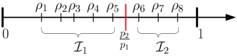
Figure 4: The Division of Advertisers

After initial price $p_{1}$ and $p_{2}$ are set in the market, the advertisers set is divided into $\mathcal{I}_{1}$ and $\mathcal{I}_{2}$. Then each search engine can compute its optimal price ${p}^{*}_{1}(\mathcal{I}_{1})$ and ${p}^{*}_{2}(\mathcal{I}_{2})$ independently as the monopoly case and price ratio $\frac{{p}^{*}_{2}(\mathcal{I}_{2})}{{p}^{*}_{1}(\mathcal{I}_{1})}$ gets updated. If it happens that the new price ratio divides the advertisers set into $\mathcal{I}_{1}$ and $\mathcal{I}_{2}$, we say this is a Nash equilibrium (NE) price pair as $(p_{1}^{NE},p_{2}^{NE})$ and neither search engine has incentive to deviate unilaterally. Otherwise, the process will iterate until the prices become stable.

Defining first the set of advertisers who participate the advertising campaign as follows.

$$\mathcal{I}_{1}^{+}(p_{1},p_{2}) \triangleq \{i\in\mathcal{I}:\rho_{i}\leq\frac{p_{2}}{p_{1}},v_{i}\geq p_{1}\}$$ (19)

$$\mathcal{I}_{2}^{+}(p_{1},p_{2}) \triangleq \{i\in\mathcal{I}:\rho_{i}>\frac{p_{2}}{p_{1}},\rho_{i}v_{i}\geq p_{2}\}$$ (20)

We now give the formal definition of NE price pair.

Definition 1.

A price pair of $(p_{1},p_{2})$ is called a Nash equilibrium price pair if $p_{1}=p^{*}(\mathcal{I}_{1}^{+}(p_{1},p_{2}))$ and $p_{2}=p^{*}(\mathcal{I}_{2}^{+}(p_{1},p_{2}))$ where $p^{*}(\mathcal{I})$ is computed according to algorithm 1.

It’s easy to see that under the NE price pair $(p_{1},p_{2})$, for any advertiser $i\in\mathcal{I}_{1}^{+}$ or $i\in\mathcal{I}_{2}^{+}$, it would have no incentive to switch to the other search engine; for advertiser $i\in\mathcal{I}_{1}\backslash\mathcal{I}_{1}^{+}$, since $\rho_{i}\leq\frac{p_{2}}{p_{1}}$ and $v_{i}<p_{1}$, it holds that $\rho_{i}v_{i}<p_{2}$, thus $i$ would not switch to engine 2 which generates zero utility according to equation (17); for advertiser $i\in\mathcal{I}_{2}\backslash\mathcal{I}_{2}^{+}$, since $\rho_{i}>\frac{p_{2}}{p_{1}}$ and $\rho_{i}v_{i}<p_{2}$, we have $v_{i}<p_{1}$ so $i$ have no incentive to switch to engine 1. Thus the NE price pair would induce a stable state to the competition system.

Proposition 3.

None-zero NE price pairs may not exist.

A simple counter-example to illustrate proposition 3 is when there is only one advertiser in the system. No matter which search engine this advertiser chooses, the price in the other search engine would be zero since it attracts no advertisers. Then the advertiser would have incentive to join the other search engine due to the zero price. However, once the advertiser switches, the price in the other search engine would become positive and price in the original engine decreases to zero. Thus the advertiser would keep switching between two search engines and no stable prices can be reached.

Proposition 4.

If NE price pair $(p_{1}^{NE},p_{2}^{NE})$ exists, it must be $p_{1}^{NE}\geq p_{2}^{NE}$.

Proof.

Assuming $p_{1}^{NE}<p_{2}^{NE}$, then since $\frac{p_{2}^{NE}}{p_{1}^{NE}}>1$, we have $\mathcal{I}_{2}^{+}(p_{1},p_{2})=\varnothing$. Therefore $p_{2}^{NE}=0$ and $p_{1}^{NE}<0$. However, it cannot be the case since rational search engine would never set negative prices. ∎

Proposition 5.

In the stable state, search engine 2 cannot make higher revenue than engine 1.

Proof.

Since $R_{1}=p_{1}^{NE}\cdot S_{1}$ and $R_{2}=p_{2}^{NE}\cdot S_{2}$, from proposition 4 and $S_{1}\geq S_{2}$, it’s easy to see that $R_{1}\geq R_{2}$. ∎

Denote $\nu$ as the price ratio $\frac{p_{2}}{p_{1}}$ which determines advertisers’ preferences, we define the optimal price ratio as:

$$f(\nu)=\frac{p_{2}^{*}(\mathcal{I}_{2}(\nu))}{p_{1}^{*}(\mathcal{I}_{1}(\nu))}$$

where $p^{*}(\mathcal{I})$ is obtained according to algorithm 1. If the advertiser partitions generated by $\nu$ are the same as those generated by the optimal price ratio $f(\nu)$, then the partitions are stable and the optimal prices become NE price pair. The problem reduces to find the fixed points which satisfy $f(\nu^{*})=\nu^{*}$. Notice that $f(\nu)$ is piece-wise constant and its value changes at $\nu=\rho_{i}$, $i\in\{1,\ldots,m\}$.

From the definitions of $\mathcal{I}_{1}$ and $\mathcal{I}_{2}$ we see that as $\nu$ increases, the preferred set of $\mathcal{I}_{1}$ would expand while $\mathcal{I}_{2}$ shrinks. According to lemma 1, we know that $p_{1}^{*}$ would increase while $p_{2}^{*}$ decreases. Therefore $f(\nu)$ should be a non-increasing function of $\nu$.

We can now show the dynamics of function $f(\nu)$ in figure 5. In this example we assume there are five advertisers re-ordered by their values of $\rho$ such that $\rho_{i}\leq\rho_{i+1}$, $i\in\{1,2,3,4\}$. Similarly, there may be two different scenarios for the location of fixed point $v^{*}$: (a) $v^{*}\in(\rho_{i},\rho_{i+1})$, $i\in\{1,\ldots,m-1\}$ as shown in figure 5a, and (b) $v^{*}=\rho_{i}$, $i\in\{1,\ldots,m\}$ as shown in figure 5b.

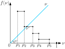
(a) Determined Division

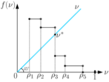
(b) Undetermined Division

Figure 5: Division of Advertisers Set by their Preferences

For case (a), the optimal $\nu^{*}$ divides the advertisers set into exactly two subsets, and all advertisers with strict preferences over certain search engine are aggregated to one of the subsets. The market would become stable after each search engine sets their optimal price. For case (b), however, there is one special advertiser who would keep switching from one search engine to the other. To illustrate it, assuming the index of this special advertiser is $l$ which satisfies the following condition:

$$\frac{p_{2}^{*}(\{l,l+1,\ldots,m\})}{p_{1}^{*}(\{1,2,\ldots,l-1\})}>\rho_{l}>\frac{p_{2}^{*}(\{l+1,\ldots,m\})}{p_{1}^{*}(\{1,2,\ldots,l\})}$$

The first inequality above implies that advertiser $l$ prefers search engine 1 if $l$ has already joined the system of search engine 2, while the second inequality implies that he would prefer engine 2 if he is associated with engine 1. Therefore, advertiser $l$ would keep switching between two search engines. In this case, we call advertiser $l$ as the undetermined advertiser.

The undetermined advertiser problem arises from our assumption that advertisers can only purchase service from one engine. This resembles the classic oscillation problem in the multi-path routing when all traffic is aggregated to the least congested path [17]. Similar to the “splittable” model in [18] where network users are permitted to route traffic fractionally over many paths, we can also make the following assumption for our model:

Assumption 1.

Splittable Budgets: We assume advertisers can arbitrarily split their budgets and invest them into both search engines to maximize their utility.

Under this splittable assumption, the dynamics of undetermined advertiser $l$’s strategic behavior could be interpreted as follows: assuming starting from the initial state where advertiser $l$ has joined engine 1, and is facing a lower price ratio ($\frac{p_{2}}{p_{1}}<\rho_{l}$) which indicates him to invest more on engine 2; then $l$ would try to split his budget into two parts: $(1-\alpha)B_{l}$ goes to engine 1 and the rest of $\alpha B_{l}$ goes to engine 2, with $\alpha\in[0,1]$. As advertiser $l$ invests more and more budgets on engine 2, i.e., $\alpha$ keeps growing from zero to one, the price ratio $\frac{p_{2}}{p_{1}}$ would keep rising until at certain $\alpha^{*}\in(0,1)$ it equals $\rho_{l}$ and advertiser $l$ would have no incentive to invest more on engine 2.

It remains to be shown whether the price ratio above would increase “smoothly” as $\alpha$ increases and whether there always exists $\alpha^{*}$ for the undetermined advertiser to divide his budget. We summarize our conclusion in the following theorem.

Theorem 2.

Assuming that there exists an undetermined advertiser $l$ and this advertiser can purchase service from both search engines. In particular, advertiser $l$ can arbitrarily split his budget into $(1-\alpha)B_{l}$ and $\alpha B_{l}$ with $\alpha\in[0,1]$, where the former is invested to engine 1 and the latter to engine 2. Then there must exist $p_{1}^{*}$, $p_{2}^{*}$ and $\alpha^{*}\in[0,1]$ such that $\frac{p_{2}^{*}}{p_{1}^{*}}=\rho_{l}$.

Proof.

Denote $\mathcal{I}_{1}\triangleq\{1,2,\ldots,l-1\}$ and $\mathcal{I}_{2}\triangleq\{l+1,l+2,\ldots,m\}$. By previous analysis we know that advertisers in $\mathcal{I}_{1}$ would always be associated with engine 1 and advertisers in $\mathcal{I}_{2}$ be associated with engine 2. It remains to be shown the effect of advertiser $l$’s splitting decision on the price ratio. Define first that $p_{1}^{0}=p_{1}^{*}(\mathcal{I}_{1})$, $p_{1}^{1}=p_{1}^{*}(\mathcal{I}_{1}\cup\{l\})$ and $p_{1}^{\alpha}=p_{1}^{*}(\mathcal{I}_{1}\cup\alpha\{l\})$ where $\alpha\{l\}$ denotes that advertiser $l$ participates in search engine 1, but with fractional budget of $\alpha B_{i}$; similarly, we define $p_{2}^{0}=p_{2}^{*}(\mathcal{I}_{2})$, $p_{2}^{1}=p_{2}^{*}(\mathcal{I}_{2}\cup\{l\})$ and $p_{2}^{\alpha}=p_{2}^{*}(\mathcal{I}_{2}\cup\alpha\{l\})$.

To prove that $\frac{p_{2}^{\alpha}}{p_{1}^{1-\alpha}}$ changes continuously from $\frac{p_{2}^{0}}{p_{1}^{1}}$ to $\frac{p_{2}^{1}}{p_{1}^{0}}$ as $\alpha$ increases from zero to one, we first present lemma 5 as follows.

Lemma 5.

Given a monopolistic search engine and the advertisers set $\mathcal{I}$. Assuming all parameters of the ad system, including engine’s supply, advertisers’ values and budgets, are definite except the budget $B_{i}$ of certain advertiser $i\in\mathcal{I}$, then the optimal price $p^{*}(\mathcal{I})$ can be regarded as a function over the variable $B_{i}\geq 0$. Furthermore, the function is continuous and non-decreasing as $B_{i}$ increases.

Proof.

Since from algorithm 1, for each realization of $B_{i}$, we can compute a definite value of optimal price, the optimal price can therefore be regarded as a function of $B_{i}$.

The property of non-decreasing (or weakly increasing) is easy to see by contradiction. Assuming for $B_{i}$ the optimal price is $p_{1}$ and for $B_{i}+\delta$ ($\delta>0$) the optimal price is $p_{2}$ with $p_{2}<p_{1}$. Then $p_{1}$ would be the optimal solution for formulation in (10)-(14) and we let $\vec{q^{*}}$ be one of the binding optimal allocations. After we increase advertiser $i$’s budget to $B_{i}+\delta$, the previous solution combination $(p_{1},\vec{q^{*}})$ would still satisfy the constraints of the revised optimization problem since $p_{1}\cdot q_{i}^{*}\leq B_{i}\leq B_{i}+\delta$ and all other conditions remain unchanged. Since $p_{2}$ is the optimal solution for the revised problem which maximizes the objective function of $p\cdot S$, we have $p_{2}\cdot S\geq p_{1}\cdot S$, thus, $p_{2}\geq p_{1}$. This contradicts with our previous assumption of $p_{2}<p_{1}$.

We now turn to prove the property of continuity. Let $p^{*}(B_{i})$ denote the optimal price under budget $B_{i}$ and $p^{*}(B_{i}+\varepsilon)$ the optimal price under budget $B_{i}+\varepsilon$ where $\varepsilon$ is any small real number. As shown in figure 2, for arbitrary budget $B_{i}\in[0,\infty)$, there exist two different scenarios for computing the optimal price: (a) all advertisers are determined; (b) there is one undetermined advertiser. We will discuss these two cases separately as follows.

Case (a): $v_{l}<p^{*}<v_{l+1}$, $l\in\{0,1,\ldots,m-1\}$ (let $v_{0}=0$). We further consider two cases for the index of advertiser $i$ whose budget $B_{i}$ is the variable: (i) $i\leq l$; (ii) $i>l$. For type (i), since $p^{*}(B_{i})=(B_{l+1}+B_{l+2}+\cdots+B_{m})/S$, the change of $B_{i}$ would not affect the value of optimal price, therefore, we have $\lim\limits_{\varepsilon\to 0}p^{*}(B_{i}+\varepsilon)=p^{*}(B_{i})$; For type (ii), since advertiser $i$ is in the participating set, the change of $B_{i}$ does affect the optimal price. Assuming $\varepsilon$ is small enough such that $|\varepsilon|<\min\{(p^{*}-v_{l})\cdot S,(v_{l+1}-p^{*})\cdot S\}$. This condition guarantees that $p^{*}(B_{i}+\varepsilon)=p^{*}(B_{i})+\varepsilon/S$ is still in the interval of $(v_{l},v_{l+1})$. Therefore, $\lim\limits_{\varepsilon\to 0}p^{*}(B_{i}+\varepsilon)=p^{*}(B_{i})+\lim\limits_{\varepsilon\to 0}\varepsilon/S=p^{*}(B_{i})$.

Case (b): $p^{*}=v_{l}$, $l\in\{1,\ldots,m\}$ and $B_{l+1}+\cdots+B_{m}\leq v_{l}\cdot S\leq B_{l}+B_{l+1}+\cdots+B_{m}$ where advertiser $l$ would only consume part of his budget under price $v_{l}$. For $i<l$, the change of $B_{i}$ would not affect $p^{*}$, so we only need to consider the case for $i\geq l$. We now consider three possible scenarios for $v_{l}\cdot S$:

1. $B_{l+1}+\cdots+B_{m}<v_{l}\cdot S<B_{l}+B_{l+1}+\cdots+B_{m}$. Assuming $\varepsilon$ is small enough such that $|\varepsilon|<\min\{v_{l}\cdot S-(B_{l+1}+\cdots+B_{m}),B_{l}+B_{l+1}+\cdots+B_{m}-v_{l}\cdot S\}$. This condition guarantees that after $B_{i}$ has changed $\varepsilon$, $v_{l}\cdot S$ is still in the interval of $(B_{l+1}+\cdots+B_{m}+\varepsilon,B_{l}+B_{l+1}+\cdots+B_{m}+\varepsilon)$, which means that $\lim\limits_{\varepsilon\to 0}p^{*}(B_{i}+\varepsilon)=\lim\limits_{\varepsilon\to 0}v_{l}=v_{l}=p^{*}(B_{i})$;

2. $v_{l}\cdot S=B_{l+1}+\cdots+B_{m}$. When $\varepsilon$ is negative, it will be equivalent to the above case (i) and therefore we have $\lim\limits_{\varepsilon\to 0^{-}}p^{*}(B_{i}+\varepsilon)=\lim\limits_{\varepsilon\to 0^{-}}v_{l}=p^{*}(B_{i})$; when $\varepsilon$ is positive, it will be equivalent to case (a) and therefore $\lim\limits_{\varepsilon\to 0^{+}}p^{*}(B_{i}+\varepsilon)=p^{*}(B_{i})+\lim\limits_{\varepsilon\to 0^{+}}\varepsilon/S=p^{*}(B_{i})$;

3. $v_{l}\cdot S=B_{l}+B_{l+1}+\cdots+B_{m}$. When $\varepsilon$ is negative, it will be equivalent to case (a) and therefore $\lim\limits_{\varepsilon\to 0^{-}}p^{*}(B_{i}+\varepsilon)=p^{*}(B_{i})+\lim\limits_{\varepsilon\to 0^{-}}\varepsilon/S=p^{*}(B_{i})$; when $\varepsilon$ is positive, it will be equivalent to the above case (i) and therefore we have $\lim\limits_{\varepsilon\to 0^{+}}p^{*}(B_{i}+\varepsilon)=\lim\limits_{\varepsilon\to 0^{+}}v_{l}=p^{*}(B_{i})$.

Therefore now we can conclude that for any $B_{i}\in[0,\infty)$, it always holds that $\lim\limits_{\varepsilon\to 0}p^{*}(B_{i}+\varepsilon)=p^{*}(B_{i})$. So $p^{*}(B_{i})$ is a continuous function over $B_{i}\in[0,\infty)$. ∎

From lemma 5 we see that $p_{2}^{\alpha}$ is continuous and weakly increasing function of $\alpha$ and $p_{1}^{1-\alpha}$ is continuous and weakly decreasing function of $\alpha$, thus the price ratio $\frac{p_{2}^{\alpha}}{p_{1}^{1-\alpha}}$ is continuous and weakly increasing from $\frac{p_{2}^{0}}{p_{1}^{1}}$ to $\frac{p_{2}^{1}}{p_{1}^{0}}$ as $\alpha$ rises from zero to one. Thus there must exist an optimal $\alpha^{*}\in[0,1]$ such that $\frac{p_{2}^{\alpha^{*}}}{p_{1}^{1-\alpha^{*}}}=\rho_{l}\in(\frac{p_{2}^{0}}{p_{1}^{1}},\frac{p_{2}^{1}}{p_{1}^{0}})$. ∎

4.3 Comparison of Competition and Monopoly

After showing the existence of Nash equilibrium prices under a relaxed assumption, we can apply this NE outcome to predict the revenue and social welfare in the duopoly environment, and compare them with the corresponding results when one search engine monopolize the market. These comparative results would be instructive in practice considering the attempt of cooperation among large search companies such as Google and Yahoo!.

We now turn to compare the prices under competition and monopoly. The main results are given in the following theorem.

Theorem 3.

The equilibrium price in search engine 1 (or engine 2) under competition is no less (or larger) than the optimal price when engine 1 monopolizes the market.

Proof.

Assuming all discount factors are randomly drawn in the range of $(\overline{\rho},\underline{\rho})$. According to equation (1) and proposition 1, the monopoly price $p^{*}$ satisfies the following condition:

$$p^{*}\cdot S=m\cdot E(B)\cdot[1-F(p^{*})]$$ (21)

Now we divide the total supply arbitrarily into $S_{1}=\alpha S$ and $S_{2}=(1-\alpha)S$, $\alpha\in[0,1]$ for search engine 1 and 2. Suppose the optimal prices are $p_{1}$ and $p_{2}$ respectively and there are $m_{1}$ advertisers attracted by engine 1 and $m_{2}$ advertisers by engine 2 where $m_{1}+m_{2}=m$, by applying equation (1) and proposition 1 we get the following equations for both search engines,

$$p_{1}\cdot\alpha S = m_{1}\cdot{E(B)}\cdot[1-F(p_{1})]$$ (22)

$$p_{2}\cdot(1-\alpha)S = \sum_{i\in\mathcal{I}_{2}}{E(B)}\cdot\mbox{Prob}\{\rho_{i}v_{i}>p_{2}\}$$ (23)

since in equilibrium $p_{2}/p_{1}=\nu^{*}$ and for each advertiser $i\in\mathcal{I}_{2}$ it holds that $\rho_{i}\geq\nu^{*}$, we can derive that:

$$\mbox{Prob}\{\rho_{i}v_{i}>p_{2}\}=\mbox{Prob}\{\rho_{i}v_{i}>\nu^{*}p_{1}\}\geq\mbox{Prob}\{v_{i}>p_{1}\}=1-F(p_{1})$$

Now the equation (23) would become:

$$\nu^{*}(1-\alpha)\cdot p_{1}S\geq m_{2}\cdot{E(B)}\cdot[1-F(p_{1})]$$ (24)

Summing over conditions (22) and (24), we have

$$[\alpha+\nu^{*}(1-\alpha)]\cdot p_{1}S\geq m\cdot E(B)\cdot[1-F(p_{1})]$$ (25)

Since $\nu^{*}\leq 1$, we have $\alpha+\nu^{*}(1-\alpha)\leq\alpha+(1-\alpha)=1$. Defining the following function first,

$$h(p)\triangleq\frac{1-F(p)}{p}$$

which is strictly decreasing over $p$. Then by comparing conditions (21) and (25), we get

$$h(p_{1})\leq\frac{[\alpha+\nu^{*}(1-\alpha)]\cdot S}{m\cdot E(B)}\leq\frac{S}{m\cdot E(B)}=h(p^{*})$$

we can infer that $p_{1}\geq p^{*}$.

Since from proposition 4 we have $p_{1}\geq p_{2}$ and $1-F(p)$ is a monotonic decreasing function of $p$, equation (22) would become:

$$p_{2}\cdot\alpha S\leq p_{1}\cdot\alpha S\leq m_{1}\cdot{E(B)}\cdot[1-F(p_{2})]$$ (26)

And since $\rho_{i}\leq 1$ for any $i\in\mathcal{I}_{2}$, we know that:

$$\mbox{Prob}\{\rho_{i}v_{i}>p_{2}\}\leq\mbox{Prob}\{v_{i}>p_{2}\}=1-F(p_{2})$$

thus equation (23) would become:

$$p_{2}\cdot(1-\alpha)S\leq m_{2}\cdot{E(B)}\cdot[1-F(p_{2})]$$ (27)

Summing over inequalities (26) and (27), we get

$$p_{2}S\leq m\cdot{E(B)}\cdot[1-F(p_{2})]$$

So we have:

$$h(p_{2})\geq\frac{S}{m\cdot E(B)}=h(p^{*})$$

which infers that $p_{2}\leq p^{*}$.

So in general, we have that $p_{2}\leq p^{*}\leq p_{1}$. ∎

One natural question to the duopoly market is that whether the company acting as a follower would merge with the leading company in the market. To answer it, we follow the conventional way of analyzing the total revenue and social welfare under competition and monopoly. At first glance, it seems that allowing the search engine with better technology to monopolize the market would generate higher total revenue and social welfare since it can provide better service for both advertisers and end users. However, it turns out the answer depends on the specific parameters of participants in the market. We summarize the comparison results of total revenue and social welfare under competition and monopoly in the following theorem.

Theorem 4.

Whether monopoly would bring in higher total revenue and social welfare than competition depends on the specific parameters of advertisers in the advertising systems.

We can prove this theorem by constructing the counter-examples 2 and 3 as follows.

Example 2.

Suppose there are two advertisers $\{1,2\}$ participating in the advertising system. The value, budget and discount factor of each advertiser are as follows: $v_{1}=1$, $B_{1}=2$, $\rho_{1}=1$ and $v_{2}=4$, $B_{2}=2$, $\rho_{2}=0$. The total supply of advertising opportunity is $S=1$.

Under monopoly, the optimal price $p^{*}=2$ and the maximal revenue is $R(p^{*})=p^{*}\cdot S=2$. For any $p<p^{*}$, the corresponding revenue would be $R(p)=p\cdot S<p^{*}\cdot S=2$; for any $p>p^{*}$, since $v_{1}<p$ which means advertiser 1 would not attend the system, $R(p)$ is upper bounded by the budget of advertiser 2, i.e., $R(p)\leq B_{2}=2$. This analysis proves the optimality of $p^{*}$ and $R(p^{*})$.

Under competition, advertiser 1 would choose engine 2 since $\rho_{1}=1$ and advertiser 2 would choose the other engine since $\rho_{2}=0$. We equally divide the supply into two parts: $S_{1}=S_{2}=0.5$. Now in engine 1, the optimal price is $p_{1}=4$ and $R_{1}=p_{1}\cdot S_{1}=2$; in engine 2, the optimal price is $p_{2}=1$ and $R_{2}=p_{2}\cdot S_{2}=0.5$. And the price ratio $p_{2}/p_{1}=0.25$ is less than $\rho_{1}$ and greater than $\rho_{2}$.

Therefore in this example, the competition would bring in even higher total revenue ($R_{1}+R_{2}=2.5$) than the monopoly ($R(p^{*})=2$).

Example 3.

There are still two advertisers in the system, with the following parameters: $v_{1}=2$, $B_{1}=0.75$, $\rho_{1}=0$ and $v_{2}=4$, $B_{2}=0.25$, $\rho_{2}=1$. The total supply of advertising opportunity is still $S=1$.

Under monopoly, the optimal price $p^{*}=1$ and the allocation vector is $(q_{1},q_{2})=(0.75,0.25)$. Thus the social welfare would be $SW=v_{1}q_{1}+v_{2}q_{2}=2.5$.

Under competition, advertiser 1 would choose engine 1 since $\rho_{1}=0$ and advertiser 2 would choose the other engine since $\rho_{2}=1$. We still divide the supply into $S_{1}=S_{2}=0.5$. Now in engine 1, the optimal price is $p_{1}=1.5$ and the social welfare $SW_{1}=v_{1}q_{1}=v_{1}S_{1}=0.75$; in engine 2, the optimal price is $p_{2}=0.5$ and $SW_{2}=v_{2}q_{2}=v_{2}S_{2}=2$. And the price ratio $p_{2}/p_{1}=1/3$ is greater than $\rho_{1}$ and less than $\rho_{2}$.

Therefore in this example, the competition would bring in even higher social welfare ($SW_{1}+SW_{2}=2.75$) than the monopoly ($SW=2.5$).

Theorem 4 shows that there is no common conclusion on whether the existence of an inferior company (or product) in the market would raise or drive down the social welfare (or total revenue). Our observation here based on the particular search engine competition model coincides with the finding in the recent paper [12] that the viability of differentiated services scheme depends on the specific characteristics of users in the system. The services provided by search engine 1 and engine 2 can be regarded as the 1st and 2nd class services in [12] where the 1st class is usually charged higher price than the 2nd (analogous to our proposition that $p_{1}^{NE}\geq p_{2}^{NE}$).

Recall that our conclusions above are based on the ex post perspective which includes all possible instances of the competitive market. To show the more general ex ante results under common parameter setting of participants, we conduct the simulation in the next section.

5 Simulation Results and Observations

In this section we present some simulation results showing the effects of different parameters in our model. There are four major criteria we would like to explore in the model:

1. Prices: We would like to compare the equilibrium prices of both engines with the monopoly price if there is only one search engine dominates the market. In the following section we denote $(p_{1},p_{2})$ as the duopoly prices and $p_{M}$ as the monopoly price.

2. Revenues: It would be intriguing to study the comparative results of total revenues under competition and monopoly. The gap between revenues under competition and monopoly would serve as a signal of whether the leading company would like to propose a merger or acquisition to its competitor. A huge gap would infer that reaching certain cooperation agreement between the two competitors would significantly promote the revenues for both companies.

3. Aggregate Utility of Advertisers: We compare the aggregate utility of advertisers to see whether monopoly would be detrimental to the interest of advertisers, and if so, how severe the loss would be. In particular, we examine the aggregate utility for brand advertisers who benefits from the relatively lower price of the inferior search engine in the duopoly market.

4. Social Welfare: Social welfare can be regarded as the realized value of advertisers and is the benchmark for addressing the interest of the community as a whole. Under competition, the social welfare is computed according to the following equation:

   $$SW=\sum_{i\in\mathcal{I}_{1}}v_{i}q_{i}+\sum_{i\in\mathcal{I}_{2}}\rho_{i}v_{i}q_{i}.$$ (28)

   where $q_{i}$ is amount of supply allocated to advertiser $i$.

In the following, we carry out a set of simulation to investigate the comparative results under different parameter settings. For each simulation setting, we randomly generate 5000 instances of parameters and calculate the average value of each criterion. The expected values from ex ante perspective can then be approximated by the average values of large amounts of ex post instances.

(1). Baseline Setting:

We consider two search engines equally dividing the market and the total supply is normalized to unity. Thus the supply of either search engine is $S_{1}=S_{2}=0.5$. Advertisers’ values are uniformly distributed over $(18,20)$, and their budgets are also drawn from uniform distribution with expectation $E(B)=4$. Discount factors of advertisers are uniformly distributed over $(0.5,0.9)$. Therefore there would be expectedly one half of advertisers with discount factors larger than the average value $E(\rho)=0.7$, which we define as the brand advertisers.

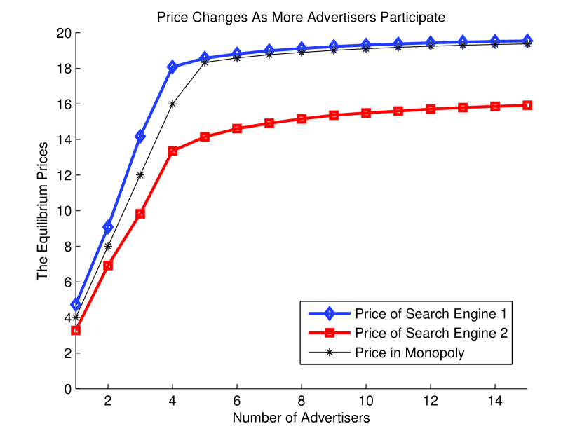
(a) Prices

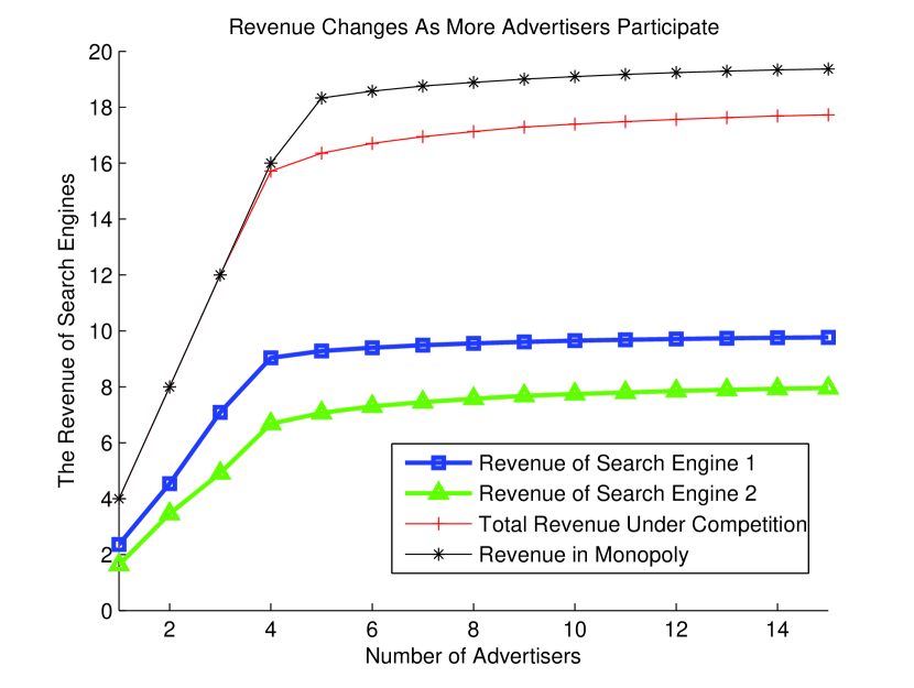
(b) Revenues

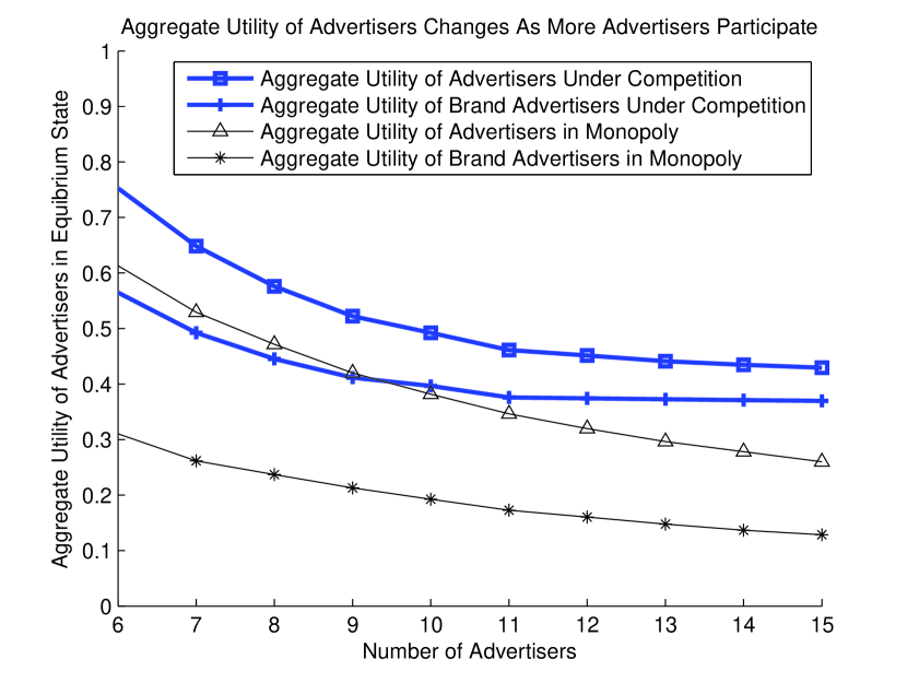
(c) Aggregate Utility of Advertisers

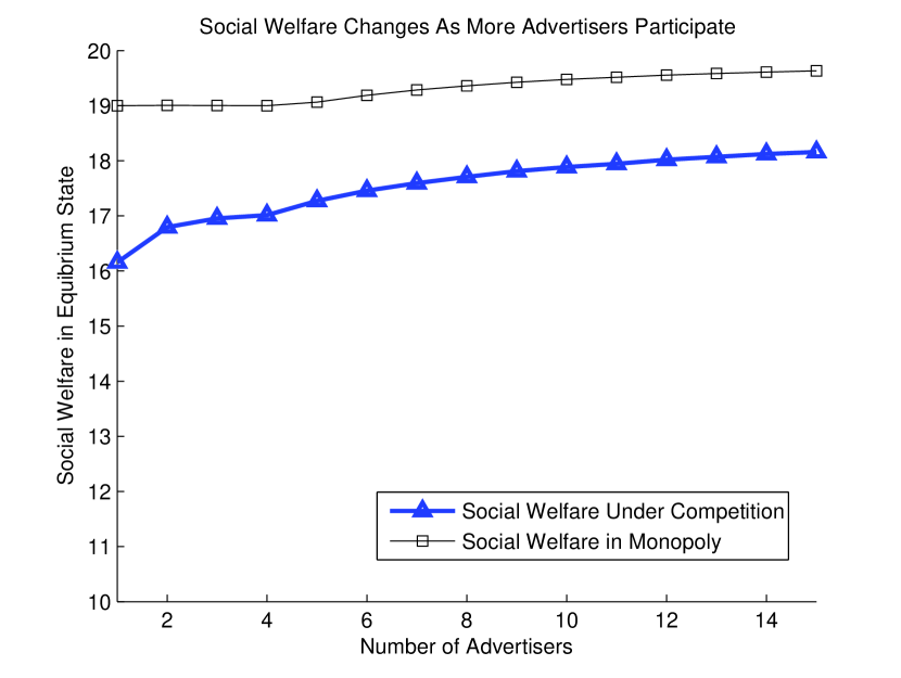
(d) Social Welfare

Figure 6: Baseline Setting

The simulation results under baseline setting are presented in figure 6. We can make the following observations from figure 6(a)-(d):

1. As the number of advertisers increases, the prices, revenues and social welfare would all get raised except the aggregate utility of advertisers. This is because as more advertisers participate, the demand for the limited supply would get boosted, which would finally drive up the unit price per supply and raise the revenue of search engines. As the price rises, the utility of advertisers would keep decreasing as seen in figure 6(c). The social welfare can still be improved since when more advertisers appears, only those advertisers with higher values can stay and be allocated with certain amount of supply. Thus the realized values of advertisers would be larger and the social welfare get enhanced.

2. After the number of advertisers reaches about five, the growth of prices and revenues seems saturated: more advertisers would not bring evident enhancement in prices and revenues. This can be derived from our parameter setting: $E(B)/E(v)=4/19\thickapprox 0.2$ is the approximate amount of demand for each advertiser, and since the total supply is one, in expectation it would be sufficient for five advertisers to consume all the supply.

3. Figure 6(a) corresponds with theorem 3 that the monopoly price is smaller than the duopoly price $p_{1}$ of engine 1 and larger than price $p_{2}$ of engine 2. We further notice that the monopoly price is actually very close to $p_{1}$ but $p_{2}$ is much smaller than $p_{1}$. This is because the monopoly engine and engine 1 in competition face advertisers with the same distribution of values. Recall that value is the maximal willingness to pay for advertisers, thus when there are too many advertisers competing with each other, the price would approach the maximal possible value, which is $20$ according to the distribution range. However, for search engine 2, the actual values of advertisers are the original values discounted by $\rho$. The lower $\rho$ is, the larger the gap between $p_{1}$ and $p_{2}$ would be.

4. Figure 6(b) shows that revenue of search engine 1 is larger than that of engine 2. This can be easily deducted since the revenue of each engine is $R_{1}=p_{1}\cdot S_{1}$, $R_{2}=p_{2}\cdot S_{2}$ and we have $p_{1}>p_{2}$, $S_{1}=S_{2}$. As we have mentioned, the monopoly price $p_{M}$ is approximately equal to $p_{1}$. Therefore the monopoly revenue can be denoted as follows:

   $$R_{M} = p_{M}\cdot S\thickapprox p_{1}\cdot S=p_{1}\cdot S_{1}+p_{1}\cdot S_{2}$$ (29)

   $$= R_{1}+\frac{p_{1}}{p_{2}}R_{2}=R_{1}+\frac{R_{2}}{\rho^{*}}>R_{1}+R_{2}$$

   where $\rho^{*}$ is the discount factor of the indifferent advertisers which is always less than one. This inequality explains the gap between total revenue under competition and monopoly in figure 6(b).

5. The utility of advertisers depends on two factors: the value and the price. Compared with the monopoly, under competition a portion of advertisers could enjoy a relatively lower price which would result in higher utility; at the same time, due to the effect of $\rho$, the values of advertisers in engine 2 get discounted which would cause lower utility. When the positive factor of lower price dominate the negative factor of lower value, the utility under competition would be greater and vice versa. Since in our baseline setting we set a relatively large $\rho$, the negative factor would be small and advertisers in engine 2 can benefit from the lower price. This conjecture can be verified in figure 6(c). Since in average brand advertisers account for half of all advertisers, in monopoly the utility of brand advertisers is always half of the utility of all advertisers as shown in figure 6(c). However, under competition the brand advertisers would benefit more than the rest advertisers since they have higher discount factors which means lower negative effect on values but confronting a lower price in engine 2.

6. Figure 6(d) indicates that the social welfare under competition is lower than that under monopoly since the realized values in equation (28) get discounted due to the factor $\rho$.

(2). Effect of Supplies

We now change the supplies to $S_{1}=0.9$ and $S_{2}=0.1$ while all other parameters remain the same. The simulation results are presented in figure 7.

In this setting one search engine plays the leading role in the market and the follower can only take a small fraction of market share. This assumption is more realistic considering the current dominant position of Google in most areas of the world. Figure 7(a) shows little difference with the corresponding price curves in figure 6(a) since all prices approach the maximal possible value when there are sufficient number of advertisers in the market. Since the supply of engine 2 decreases, the revenue of engine 2 which is denoted by $R_{2}=p_{2}\cdot S_{2}$ would also drop. According to equation (29), the gap of the total revenues is $R_{M}-(R_{1}+R_{2})\thickapprox(\frac{1}{\rho^{*}}-1)R_{2}$. Therefore when $R_{2}$ is small, the gap would also be negligible. This is verified by figure 7(b). This result also demonstrates that even when the follower takes a small portion of market share and provides service of relatively lower quality, it can still make nontrivial profit through competition and survive in the market. In figure 7(c), the gain of aggregate utility under competition is tiny compared with that under monopoly since engine 2 can only provide limited supply (10% of the total supply) and only very few of advertisers can take advantage of it. Figure 7(d) shows that the loss of social welfare under competition is very small since only 10% of the total supply is of lower quality, i.e., the second term in equation (28) is insignificant.

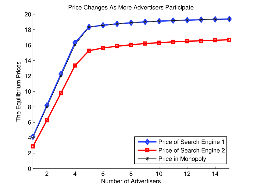
(a) Prices

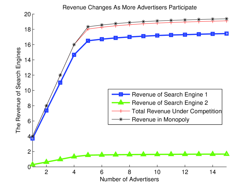
(b) Revenues

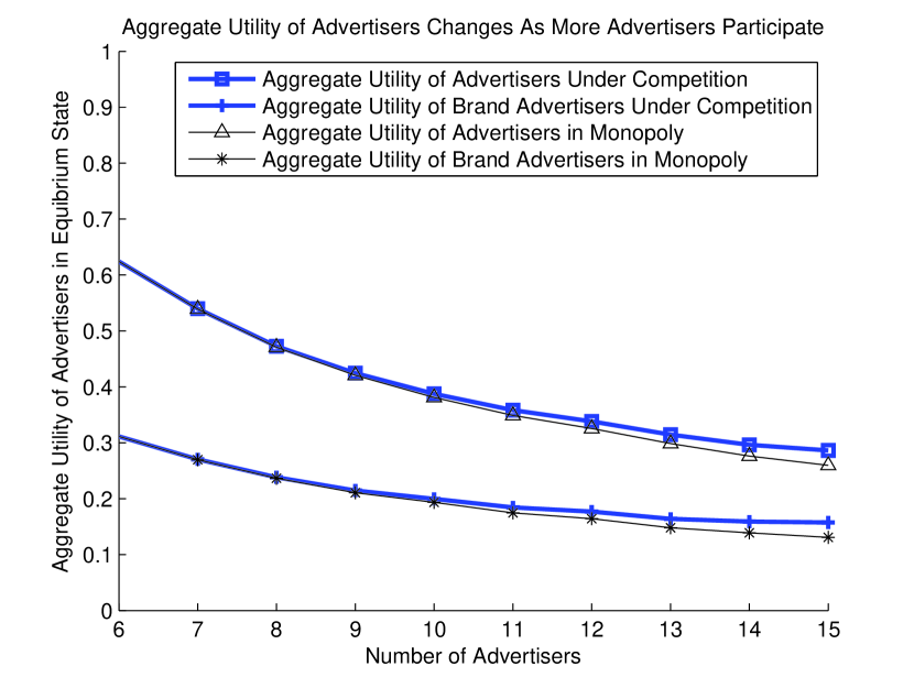
(c) Aggregate Utility of Advertisers

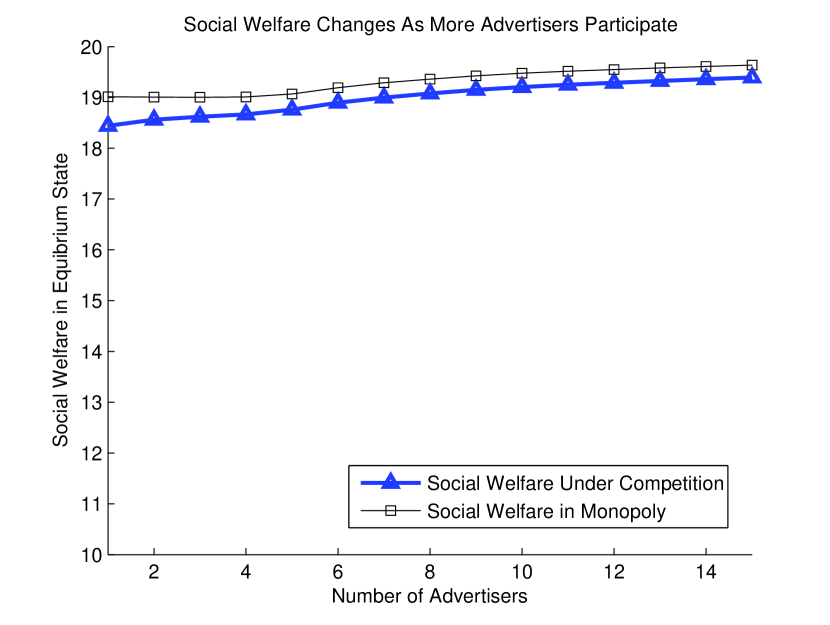
(d) Social Welfare

Figure 7: When Supplies Change To $S_{1}:S_{2}=9:1$

(3). Effect of Discount Factors

We now turn to investigate the effect of technology gap between two search engines. Let the discount factors be drawn uniformly on $(0.1,0.5)$ and all other parameters are the same as the baseline setting.

As figure 8(a) shows, the equilibrium price $p_{1}$ of engine 1 and the monopoly price $p_{M}$ are still close to the maximal value of advertisers and $p_{2}$ approaches the maximal discounted value $\rho v$. As $\rho$ decreases, the price of engine 2 also diminishes compared with $p_{2}$ in figure 6(a) and 7(a).

Since the revenue $R=p\cdot S$ and from above analysis we know $p_{1}$ has little change and $p_{2}$ diminishes, the revenue $R_{1}$ of engine 1 would stay almost the same while $R_{2}$ reduces as shown in figure 8(b). Since we have also mentioned that the gap between the total revenues approximates to $R_{M}-(R_{1}+R_{2})\thickapprox(\frac{1}{\rho^{*}}-1)R_{2}$, when $\rho$ is small, the gap would become larger. This can be easily seen by comparing the corresponding revenue curves in figure 6(b) and figure 8(b).

The aggregate utilities of advertisers in monopoly are the same in figure 6(c) and figure 8(c); however, the aggregate utilities under competition in figure 8(c) is much smaller than those in figure 6(c) due to the negative effect of $\rho$ on advertisers’ values. In figure 8(c) we see that there is certain intersection between utility under competition and monopoly. When there are only a few of advertisers, the prices are still low and the main factor affecting utility is the value. Under competition the existence of $\rho$ would drive down advertisers’ values and thereby results in lower aggregate utility. As the number of advertisers increases, the monopoly price $p_{M}$ would approach the maximal value $v_{max}=20$ and the aggregate utility would gradually reduce to zero. However, even when $p_{1}$ and $p_{M}$ approach $20$, the rest of advertisers whose discount factors are larger than the equilibrium price ratio $\rho^{*}=p_{2}/p_{1}$ can still obtain nontrivial utility which can be approximated as $(\bar{\rho}v-p_{2})S_{2}\thickapprox(\bar{\rho}v-\rho^{*}v)S_{2}$ ($\bar{\rho}$ denotes the average value of advertisers with discount factors larger than the price ratio $\rho^{*}$).

Figure 8(d) displays the hug gap between social welfare under competition and monopoly. Since half of the supply ($S_{2}=0.5$) is allocated to advertisers with discount factors less than $0.5$, the realized values in equation (28) would become significantly smaller than social welfare under monopoly.

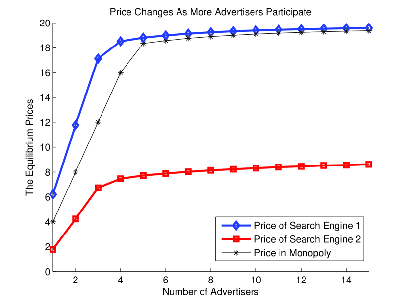
(a) Prices

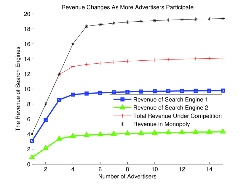
(b) Revenues

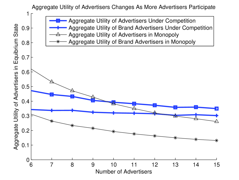
(c) Aggregate Utility of Advertisers

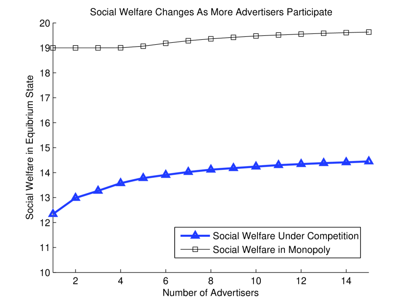
(d) Social Welfare

Figure 8: When $\rho$ Belongs to $(0.1,0.5)$

6 Conclusion and Future Work

We propose an analytical framework to model the interaction of publishers, advertisers and users under monopoly and duopoly scenarios. For monopoly market, we can give the analytical results of price and revenue for both ex ante and ex post case. For duopoly market, we formulate a three-stage dynamic game to model the search engines’ competition for both users and advertisers and prove the existence of Nash equilibrium from ex post perspective. To see the long-term effect of competition from ex ante perspective, we carry out computer simulations for different settings of participants’ parameters. The comparative results of revenues and social welfare under competition and monopoly are then presented and discussed extensively in the paper. Our analysis could provide some insight in regulating the search engine market and protecting the interests of advertisers and end users. Although the cooperation between search engines can probably bring more total revenues, advertisers and users may be averse to such plan which eliminates their freedom to choose from diverse services provided by different search companies.

There are several possible ways to extend our work. Throughout our paper, we implicitly assume that advertisers would reveal their true parameters such as values and budgets to the search engines. Since our framework is by no means strategy-proof, how would rational advertisers’ strategies affect our conclusions would be an interesting question for further investigation. Another non-trivial problem is how to associate our analytical result of revenue from one particular keyword with the practical revenue of an industrial search company which gathers from numerous keywords queried by end users everyday. Besides, to be in line with the practical advertising system nowadays, we will consider incorporating the quality factor of advertisement for the revenue-ranking rule as well as the generalized second-price auction prevailing in major search engines. Finally, it would be intriguing to extend our model for multiple search engines scenario besides the basic duopoly scenario.

References

- [1] Interactive Advertising Bureau, “IAB Internet Advertising Revenue Report,” April 7, 2010. Available Online: http://www.iab.net/media/file/IAB-Ad-Revenue-Full-Year-2009.pdf.
- [2] B. Jansen and T. Mullen, “Sponsored Search: An Overivew of the Concept, History, and Technology,” Int. J. Electronic Business Vol. 6, No. 2, pages 114 - 131, 2008.
- [3] L. Ausubel, “An Efficient Ascending-Bid Auction for Multiple Objects,” American Economic Review 94(5), pages 1452 - 1475, Dec 2004.
- [4] R. Pollock, “Is Google The Next Microsoft? Competition, Welfare and Regulation in Internet Search,” Cambridge Working Papers in Economics, April 2009.
- [5] G. Sapi and I. Suleymanova, “Beef Up Your Competitor: A Model of Advertising Cooperation Between Internet Search Engines,” DIW Berlin Discussion Paper No. 870, March 2009.
- [6] S. Lahaie, D. Pennock, A. Saberi, R. Vohra, “Sponsored Search Auctions,” Chapter 28 of Algorithm Game Theory, Cambridge University Press, pages 699 - 715, Sep 2007.
- [7] H. Hotelling, “Stability in Competition,” Economic Journal 39, pages 41 - 57, 1929.
- [8] S. Anderson, J. Goeree and R. Ramer, “Location, Location, Location,” Journal of Economic Theory 77, pages 102 - 127, 1997.
- [9] M. Frutos, H. Hamoudi, X. Jarque, “Equilibrium Existence In The Circle Model with Linear Quadratic Transport Cost,” Regional Science and Urban Economics 29, pages 605 - 615, 1999.
- [10] S. Brenner, “Determinants of Product Differentiation: A Survey,” Humboldt University, Mimeo, 2001.
- [11] M. Benisch, N. Sadeh, T. Sandholm, “Methodology for Designing Reasonably Expressive Mechanisms with Application to Ad Auctions,” IJCAI-09, pages 46 - 52, 2009.
- [12] C. Chau, Q. Wang, D. Chiu, “On the Viability of Paris Metro Pricing for Communication and Service Networks,” IEEE INFOCOM 2010, pages 1 - 9, March 2010.
- [13] B. Edelman, M. Ostrovsky, M. Schwarz, “Internet Advertising and the Generalized Second-Price Auction: Selling Billions of Dollars Worth of Keywords,” American Economic Review 97(1), pages 242 - 259, March 2007.
- [14] H. Varian, “Position Auctions,” International Journal of Industrial Organization 25, pages 1163 - 1178, 2007.
- [15] I. Ashlagi, D. Monderer, M. Tennenholtz, “Competing Ad Auctions,” Fourth Workshop on Ad Auctions, Chicago, July 2008.
- [16] D. Liu, J. Chen, A. Whinston, “Competing Keyword Auctions,” Fourth Workshop on Ad Auctions, Chicago, July 2008.
- [17] J. He and J. Rexford, “Towards Internet-wide Multipath Routing,” IEEE Network Magazine 22(2), pages 16 - 21, March 2008.
- [18] T. Roughgarden and É. Tardos, “How Bad Is Selfish Routing?” JACM 49(2), pages 236 - 259, 2002.
- [19] C. Borgs, J. Chayes, N. Immorlica, M. Mahdian, A. Saberi, “Multi-unit Auctions with Budget-constrained Bidders,” EC’05, Vancouver, June 2005.
- [20] G. Aggarwal, A. Goel, R. Motwani, “Truthful Auctions for Pricing Search Keywords,” EC’06, Michigan, June 2006.
- [21] Y. Zhou, R. Lukose, “Vindictive Bidding in Keyword Auctions,” EC’07, Minnesota, August 2007.
- [22] A. Goel, K. Munagala, “Hybrid Keyword Search Auctions,” WWW’09, Madrid, April 2009.
- [23] D. Martin, J. Gehrke, J. Halpern, “Toward Expressive and Scalable Sponsored Search Auction,” International Conference on Data Engineering, pages 237 - 246, 2008.
- [24] E. Dar, M. Kearns, J. Wortman, “Sponsored Search with Contexts,” WINE 2007, pages 312 - 317, 2007.
- [25] Z. Abrams, A. Ghosh, E. Vee, “Cost of Conciseness in Sponsored Search Auctions,” WINE 2007, pages 326 - 334, 2007.
- [26] D. Kempe, M. Mahdian, “A Cascade Model for Externalities in Sponsored Search,” Fourth Workshop on Ad Auctions, Chicago, July 2008.
- [27] G. Aggarwal, J. Feldman, S. Muthukrishnan, M. Pl, “Sponsored Search Auctions with Markovian Users,” Fourth Workshop on Ad Auctions, Chicago, July 2008.
- [28] A. Das, I. Giotis, A. Karlin, C. Mathieu, “On the Effects of Competing Advertiserments in Keyword Auctions,” EC’08, Chicago, July 2008.
- [29] A. Ghosh, A. Sayedi, “Expressive Auctions for Externalities in Online Advertising,” WWW 2010, Raleigh, April 2010.