Computational Tools for Evaluating Phylogenetic and Hierarchical Clustering Trees

Abstract.

Inferential summaries of tree estimates are useful in the setting of evolutionary biology, where phylogenetic trees have been built from DNA data since the 1960’s. In bioinformatics, psychometrics and data mining, hierarchical clustering techniques output the same mathematical objects, and practitioners have similar questions about the stability and ‘generalizability’ of these summaries. This paper provides an implementation of the geometric distance between trees developed by Billera, Holmes, and Vogtmann (2001) equally applicable to phylogenetic trees and heirarchical clustering trees, and shows some of the applications in statistical inference for which this distance can be useful.

In particular, since Billera et al. (2001) have shown that the space of trees is negatively curved (a CAT(0) space), a natural representation of a collection of trees is a tree. We compare this representation to the Euclidean approximations of treespace made available through Multidimensional Scaling of the matrix of distances between trees. We also provide applications of the distances between trees to hierarchical clustering trees constructed from microarrays. Our method gives a new way of evaluating the influence both of certain columns (positions, variables or genes) and of certain rows (whether species, observations or arrays).

1. Current Practices in Estimation and Stability of Hierarchical Trees

Trees are often used as a parameter in phylogenetic studies and for data description in hierarchical clustering and regression through procedures like CART (Breiman et al., 1984). These methods can generate many trees leading to the need for summaries and methods of analysis and display.

A natural distance between trees has been introduced and studied in Billera, Holmes, and Vogtmann (2001). Recent advances in its computation (Owen and Provan, 2009), along with advances reported below, now allow for efficient computation and use of this distance. The present paper describes these advances and some applications. We begin with a small example.
Example 1: Hierarchical Clustering variability
Now a staple of microarray visualizations, the hierarchical clustering trees such as that in Figure  1 is a standard heatmap type plot showing both a clustering of patients (the columns in this data) and the genes (the rows).

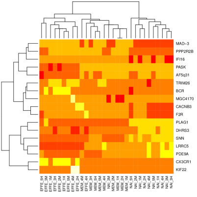
(a) Hierarchical Clustering trees of both rows and columns of a microarray matrix. Rows are genes, columns are patients.

(b) Plot of cross validated hierarchical clustering trees. Each point represents a tree that was estimated without the gene it is labeled with.

Figure 1. Cross validation of the rows allows us to geometrically study the leverage of individual genes.

We will consider using cross validation to see how the clustering trees change when each of the genes was removed. This gives us 16 cross validated trees and the original tree. These 17 points can be represented in a plane, where the groupings show that some genes have similar effects on the estimates when missing. Figure  1 shows the cross validated trees with the original tree at the center of the triangular scatter of points. Notice that the cross validated trees can be seen to form three clusters. We will explain how this plot was made in section 3.6.

1.1. Trees as Statistical Summaries

Hierarchical clustering trees and phylogenetic trees are some of the most popular graphical representations in contemporary evolutionary biology and data analysis. They share a common non-standard output: a binary rooted tree with the known entities at the leaves. Mathematicians often call them rooted semi-labeled binary trees (Semple and Steel, 2003). The trees are built from multivariate data sets with data on the leaves; we will suppose the data are organized so that each row corresponds to a leaf.

Current practices in evaluating tree estimates lean on unidimensional summaries giving the proportion of times a clade occurs. These are recorded either as the binomial success rates along the branches of the tree (Felsenstein, 1983) or as a set of bin frequencies of the competing trees considered as categorical output.

In this paper we propose alternative evaluation procedures, all based on distances between trees. The idea of comparing trees through a notion of distance between trees has many variations. Robinson and Foulds (1981) proposed a coarse distance between phylogenetic trees that takes on only integer values; Waterman and Smith (1978) proposed the Nearest Neighbor Interchange (NNI) as a biologically reasonable distance between trees. We will use that of Billera, Holmes, and Vogtmann (2001) and call it the BHV distance. This distance can be considered in some sense to be a refinement of NNI that comes from taking into account the edge lengths of the trees.

In this first section we will place the question of evaluating trees in the context of statistical estimation and give an overview of current practices in data analysis. Here our data will be presented as a $n\times p$ matrix, with n being the number of observations for the hierarcical clustering studies or the number of species for the phylogenetic examples. The elements of the matrix will mostly come from small alphabets; examples in the paper include ${\mathcal{A}}=\{0,1\},\mbox{ or }\{-1,0,1\}\mbox{ or }\{a,c,g,t\}$.

The second section will provide a short description of the algorithm for computing the distances between trees as we have implemented it. Section 3 shows how we can use multidimensional scaling to approximately embed the trees in a Euclidean space. We show examples of using multidimensional representations for comparing trees generated from different data, and for comparing cross validated data for detecting influential variables in hierarchical clustering. Section 4 shows how we embed the trees in a tree, providing a robust method for detecting mixtures. We also introduce a quantitative measure of treeness that tells us how appropriate a tree representation might be.

Section 5 shows how paths between trees can be used to find the boundary points between two different branching orders. These paths are built using simulated annealing algorithm and can also provide the boundary data used by Efron, Halloran, and Holmes (1996) to correct the bias in the naïve bootstrap for trees (Holmes, 2003).

1.2. Estimating phylogenetic trees from Data

The true tree, if one exists, can be considered an unknown parameter that we can use standard statistical estimation methods to estimate (Holmes, 1999). Recently, it has become apparent that in many cases there are probably several good candidate trees that must be presented together to explain the complexities of the evolutionary process. Having several trees to represent increases the need for a satisfactory comparison technique. We will begin, however, with the simplest case, that of having only one true tree with a simple model of evolution.

If the data are the result of a simple treelike evolutionary process, we may model the process as a Markov chain. We can characterize it by a pair of parameters $(\tau,M)$, where $\tau$ represents the tree with its edge lengths and $M$ is the mutation (transition) matrix. If the characters measured at the leaves of the tree are binary, M will be a $2\times 2$ transition matrix; in the familiar case of observed DNA, $M$ will be a $4\times 4$ transition matrix.

Example 2: Balanced phylogenetic tree and comb-like phylogenetic trees.

Figure 2. Two common representations of trees. The dendrogram representation of a balanced tree with 17 leaves is on the left, the cladogram representation of the same tree is on the right.

On the right, the cladogram is often considered a useful representation of an evolutionary process, where the root represents the common ancestor to the 17 leaves or taxa at the end of the tree. The simplest evolutionary process is that denoted by the Cavender-Farris-Neyman (Felsenstein, 2004) process where each position or character is binary. Suppose we consider just one character; we generate the character at the root at random, say from a fair coin. This character will then ‘evolve’ (that is, be pushed) through the tree from the root to the leaves, with some probability of mutating as it passes through edges. The mutations have a higher probability of occurring over longer branches. The simplest model for mutation is to suppose a molecular clock, and thus that the rate is the same throughout the tree and always proportional to the edge lengths. If the mutation rate is very low, we might end up with all the characters at the 17 leaves equal to the root, while if it is very high, the characters at the leaves will have very little resemblance to those at the root. The leaves usually represent the contemporary taxa and thus we can guess what was at the root by what occurs at the leaves as long as the mutation rate is neither too low nor too high.

Figure 3. The tree on the left was estimated with a matrix which had 100 columns (characters), of which only 24 different patterns are represented in the columns. The tree on the right was estimated with a matrix of 400 columns, with 68 different patterns represented. We can see that the tree on the right has the correct branching order, as compared to the estimate on the left.

Another factor that effects the tree estimation quality is tree shape. As an example, here are two trees that were used to generate data. We call the left one the comb tree and the right one the balanced tree.

Figure 4. Two theoretical trees were used to simulate sequences of length 400. The tree on the left is the comb tree, and the tree on the right is often called the balanced tree.

Figure 5. The two theoretical trees from Figure 4 were used to simulate sequences of length 400. From this example it seems the tree with the larger inner branch lengths was easier to estimate. We will make this precise in Section 3.

Tree estimation methods can be grouped into categories of parametric, non-parametric, and intermediate methods. One popular parametric estimation method is maximum likelihood (MLE) (a classical textbook presentation of this can be found in Felsenstein (2004)). Although this is known to be NP-complete, remarkable computational advances have been made in recent years with regards to this reconstruction problem and particularly efficient implementations exist, such as RAxML (Stamatakis et al., 2005) or PhyML (Guindon and Gascuel, 2003). Another parametric approach is the Bayesian Maximum A Posteriori (MAP) estimate, implemented in Mr Bayes (Huelsenbeck and Ronquist, 2001) or Beast (Drummond and Rambaut, 2007) following Yang and Rannala’s prescription for Bayesian inference and tree estimation (Yang and Rannala, 1997).

The most standard nonparametric estimate for a tree is the Maximum Parsimony tree. The reconstruction algorithm is designed to take the original data as the leaves and add extra ancestral points that minimize the number of mutations needed to explain the data. From a computational viewpoint, this is equivalent to the Steiner tree problem and is known to NP-complete (Foulds and Graham, 1982).

Intermediaries between strictly parametric methods based on a finite number of mutational rate-parameters and an evolutionary tree and the nonparametric approaches are the distance based methods. These use the parametric Markovian models to find the distances between species and then lean on various heuristic criteria to build a binary tree from these distances.

Distance based methods forfeit the use of the individual columns in favor of a simple distance between the aligned sequences, although recent work by Roch (2010) shows there might not be such an important loss in information. The distance can use any of the standard Markovian evolutionary models such as the Jukes Cantor one parameter model or Kimura two parameter model (Felsenstein, 2004), or a simple Hamming distance between sequences. Once the distances have been computed the tree building procedure can follow one of many possible heuristics. Neighbor Joining is an agglomerative (bottom up) method which is computationally inexpensive and is thus often used as a starting point for other tree estimation procedures. UPGMA or average linkage method is another such method that updates the distance between two clusters by taking the average distance between all pairs of points from the two groups (the orignal idea is explained in Michener and Sokal (1957), a standard treatment can be found in Felsenstein (2004)).

1.3. Hierarchical clustering trees

Building hierarchical clustering trees is very similar to the use of distances to build phylogenetic trees, with the difference that the choice of distances or even of simpler dissimilarities between the leaves is no longer driven by an evolutionary model but dissimilarities either in gene expression or in occurrence of words or other relevant features (Hartigan, 1967). The resulting hierarchical clustering has the advantage over simple clustering methods such as $k$-means that one can look at the output in order to make an informed decision as to the relevant number of clusters for a particular data set.

1.4. Methods for Evaluating Trees

In the case of hierarchical clustering trees, Fowlkes and Mallows (1983) provide a first approach to comparing two hierarchical clusterings by creating a weighted matching score from the matrix of matchings. However, recently more global distributional assessments of clusterings of trees have been possible thanks to advances in computation:

Bootstrap support for Phylogenies:

As in the standard bootstrap technique Efron (1979), with observations being the columns of the aligned sequences, the sampling distribution of the estimated tree is estimated by resampling with replacement among the characters or columns of the data. This provides a large set of plausible clusterings. These were used for instance by Felsenstein (1983) to build a confidence statement relevant to each split. An adjustment was proposed in Efron et al. (1996). This is based on finding a path between trees that are each side of the boundary separating two tree topologies; we show in Section 4 how this can be implemented using our implementation of the geometric distance.

Parametric Bootstrapping for Microarray Clusters:

Kerr and Churchill (2001) have proposed a way of validating hierarchical clustering as it is used in microarray analysis. Their model is a parametric ANOVA model for microarrays which includes gene, dye and array effects. Once these effects have been estimated on the data, simulated data incorporate realistic noise distributions can be generated through a parametric bootstrap type procedure. From the simulated data many hierarchical clusters are generated and then compared. The authors use this to evaluate the stability of a gene, using percent of bootstrap clusterings in which it matches to the same cluster in the same way Felsenstein (1983) provides the estimate of the binomial proportion of trees with a given clade. We can repeat their generation process but again combine the trees differently than by estimating a presence-absence estimate for each clade. We show in section 3 how a more multivariate approach can provide richer visualizations of the stability of hierarchical clustering trees.

Bayesian posterior distributions for phylogenetic trees:

Yang and Rannala (1997) develop the Bayesian framework for estimating phylogenetic trees using a Bayesian posterior probability distribution to assess stability. The usual models put prior distributions on the rates and a uniform distribution on the original tree and then proceed through the use of MCMC to generate instances of the posterior distribution. Since implementations such as Huelsenbeck and Ronquist (2001) provides a sample of trees from the posterior distribution, these can be used for the same purpose as the bootstrap resample of trees. Following procedures exposed in section 3, we can combine these picks from the posterior distribution using the distances to give an estimate of a median posterior tree and to give multivariate representations such as hierarchical clusters and MDS plots of the posterior distribution.

Bayesian methods in hierarchical clustering:

Savage et al. (2009) provide a Bayesian nonparametric method for generating posterior distributions of hierarchical clustering trees. Visualizing such posterior distributions can be tackled with the same tools as those used for Bayesian phylogenetics.

2. The Polynomial Time Geodesic Path Algorithm

2.1. Path Spaces, Geodesics, and Uniqueness

The distance algorithm implemented computes the geodesic distance metric proposed by Billera, Holmes, and Vogtmann (2001). This arises naturally from their formulation of tree space as a space made up of Euclidean orthants. A path between two trees consists of line segments through a sequence of orthants. This sequence of orthants is the path space. A path is a geodesic when it has the smallest length of all paths between two points.

As Billera, Holmes, and Vogtmann (2001) showed, tree space is a negatively curved CAT(0) space. As a consequence, there is a unique geodesic between any two trees (Gromov, 1987). We then can find the distance between two trees by finding the geodesic path.

2.2. The Algorithm Intuitively

Owen and Provan (2009) have proposed an iterative method to constrict a path until it is the geodesic between its two endpoints. Since all orthants connect at the origin, any two trees $T$ and $T^{\prime}$ can be connected by a two-segment path, consisting of one segment from $T$ to the origin, and another from the origin to $T^{\prime}$. This path is in general not a geodesic, but is an easily definable path that must always be valid, making it a useful starting point. This path is called the cone path.

From this start, the algorithm iteratively splits a transition between orthants into two transitions by introducing a new itermediate orthant into the path space until a condition is met such that we know the path is the geodesic. We then compute the length of the path to get the geodesic distance between the two trees.

2.3. Notation and Setup

Let $T$ and $T^{\prime}$ be two rooted semi-labeled weighted binary trees with $n$ labeled tips, with labels $X=1..n$, and $2n-2$ edges $\mathcal{E}$ and $\mathcal{E}^{\prime}$. Formally, we hang the trees by a labeled root $Z$, though because of a representational trick it is not necessary to include this in the computations. Every edge $e\in\mathcal{E}$ defines a partition of labels $X_{e}|\overline{X}_{e}$. As a convention we will consider $X_{e}$ as the set of labels ‘below’ $e$ (that is, the set not including $Z$), and $\overline{X}_{e}$ as the set of edges ‘above’ or ‘rootward’ of $e$, or the set containing $Z$.

Two edges $e$ and $f$ are called compatible if one of $X_{e}\cap X_{f}$, $X_{e}\cap\overline{X}_{f}$, $\overline{X}_{e}\cap X_{f}$, or $\overline{X}_{e}\cap\overline{X}_{f}$ is empty. Intuitively, edges are incompatible if they could not both be edges in the same tree. The partition formed by an edge uniquely identifies it amongst all edges in $n$-trees, so we represent each edge by the partition it forms, and call two edges the same if they form the same partition of $X$. Two sets of edges $A$,$B$ are compatible if for every $e\in A$, $e$ is compatible with every $f\in B$.

We represent a path between two trees by $(\mathcal{A},\mathcal{B})$ with $\mathcal{A}=(A_{1},...,A_{k})$ and $\mathcal{B}=(B_{1},...,B_{k})$, where $A_{i}\subseteq\mathcal{E}$ represents the edges dropped from $T$, and $B_{i}$ represents the edges added from $T^{\prime}$ at the $i^{\text{th}}$ transition between orthants. The norm $||A||$ of a set of edges is $\sqrt{\sum_{e\in A}|e|^{2}}$ where $|e|$ is the weight of $e$.

2.4. Conditions for a Path to Be a Geodesic

Owen and Provan (2009) give two properties that all valid paths must fulfill, as well as a third property that fully characterizes a geodesic path. The properties are presented here without development.

Theorem 1.

A sequence of sets of edges $(\mathcal{A},\mathcal{B})$ represents a valid path if and only if (1) for each $i>j$, $A_{i}$ and $B_{j}$ are compatible, and (2) $\frac{||A_{1}||}{||B_{1}||}\leq\frac{||A_{2}||}{||B_{2}||}\leq...\leq\frac{||A_{k}||}{||B_{k}||}$.

Theorem 2.

(Property 3) A valid path is the geodesic path if and only if, for each $(A_{i},B_{i})$ in the path, there is no partition $C_{1}\cup C_{2}$ of $A_{i}$ and partition $D_{1}\cup D_{2}$ of $B_{i}$ such that $C_{2}$ is compatible with $D_{1}$ and $\frac{||C_{1}||}{||D_{1}||}\leq\frac{||C_{2}||}{||D_{2}||}$.

Owen and Provan (2009) proved that properties (1) and (2) are always satisfied throughout the algorithm, and present a polynomial time way to both check (3) and split $(A_{i},B_{i})$ into $(A_{i},B_{i}),(A_{i+1},B_{i+1})$.

2.5. Representing Trees, Preprocessing, and Optimizations

Trees are uniquely represented by the set of partitions formed by all edges in the tree. We represent an edge by an $n+1$-length vector of logical values, a true value meaning the leaf in that position is ‘downward’ of the edge, with the $n+1$ position representing the root node $Z$. This representation allows efficient computation of edge compatibility (i.e. in O(n) time, since one iteration through the vectors can check all intersections).

Before the algorithm is implemented, several preprocessing steps are performed. There are three preprocessing steps: (1) edges are classified as shared between the two trees or unique to its own tree, (2) the trees are divided up into independently solvable subproblems, and (3) edge incompatibility information is computed and cached.

The first step, classification of edges as shared or unique, serves two purposes. Edges shared by the two trees will not get dropped or added by any transition through an orthant, and so we can think of all the shared edges as having Euclidean distance within one orthant. Since they can be added in as such at any time, there is no purpose in using them in the high-cost distance computation, and indeed the algorithm presented by Owen and Provan requires trees to be disjoint.

The second purpose this classification serves is to aid in the second preprocessing step, division into subproblems. The division works from the observation that for every shared edge in $T$,$T^{\prime}$, we can treat the distance between the subtrees from this edge as simply part of the distance between the two edges. This lets us compute the distance between these two subtrees in an identical way to the larger tree, and integrate this distance as if it were a shared edge distance.

This division is accomplished by classifying every unique edge in both trees under the tightest shared edge, i.e. working upwards until we reach a shared edge. Computationally this takes the form of, for every edge $e$, computing the difference in number of downward leaves between every shared edge and $e$, and taking the shared edge with the minimum positive difference. This approach is used since no representation of the tree as an actual binary tree is stored. The computation is still reasonably efficient due to the vector representation of the partitions and that the count of downward edges can be cached.

From the second step, we get a series of bins, each containing a pair of disjoint subtrees from a shared edge root. For each bin, we compute all pairwise edge compatibilities between edges on the two trees, caching their result in a vector of edge pairs. While these implementation details do not affect the theoretical efficiency of the algorithm, they make the computation reasonable in practice for large datasets.

2.6. The Algorithm

The algorithm itself reduces to checking property (3). Following Staple (2003), the notion of incompatibility between edges is coded into a bipartite graph. Owen and Provan show that property (3) can be checked by forming a graph $G(A_{i},B_{i})$ and computing the minimum weight vertex cover for this graph. The graph $G(A_{i},B_{i})$ is formed by adding graph edges between incompatible edges of $A_{i}$ and $B_{i}$, and weighting each vertex $v\in A_{i}$ as $\frac{||v||^{2}}{||A_{i}||^{2}}$ and $w\in B_{i}$ as $\frac{||w||^{2}}{||B_{i}||^{2}}$. Because this graph is bipartite, the minimum weight vertex cover problem can be solved using a max-flow algorithm with the following conversion: source node $s$ and sink node $t$ are added to the graph, edges are added between $s$ and every $v\in A_{i}$ with edge weight equal to the vertex weight of $v$, the edges given by incompatibilities are given infinite weight, and edges are added between every $w\in B_{i}$ and $t$ with weight equal to the vertex weight of $w$. The Edmonds-Karp max-flow algorithm was used to compute the max flow, giving a runtime complexity of $O(|V|\cdot|E|^{2})$, where $|V|=|A_{i}|+|B_{i}|+2$, and $|E|\leq|A_{i}|+|B_{i}|+|A_{i}|\cdot|B_{i}|$. For a subtree with $k$ unique edges and $n$ leaves, $|A_{i}|,|B_{i}|\leq k\leq n-2$, giving a worst-case complexity of $O(n^{3})$ for checking property (3). A breadth first search of the residual flow graph, after dropping 0-weight edges, gives the subsets $C_{1}\subset A_{i}$ and $D_{1}\subset B_{i}$ ($C_{1}\cup\overline{D_{1}}$ happens to be the minimum weight vertex cover, but at this point we don’t need the actual cover itself).

For each bin, we run the algorithm. Initialize $(\mathcal{A},\mathcal{B})$ to $A_{0}=\mathcal{E}$ and $B_{0}=\mathcal{E}^{\prime}$, that is, all edges dropped and added in one orthant transition (this is effectively the cone path of the subtree, which we know to be a valid path, satisfying properties (1) and (2)). Iteratively, we run the following procedure on all pairs $(A_{i},B_{i})$ of $(\mathcal{A},\mathcal{B})$: (1) compute the max-flow $f$ of $G(A_{i},B_{i})$ (2) if $f<1$, find all accessable edges $C_{1}\subset A_{i}$ and $D_{1}\subset B_{i}$ and replace $(A_{i},B_{i})$ with $(C_{1},D_{1}),(\overline{C_{1}},\overline{D_{1}})$ in $(\mathcal{A},\mathcal{B})$. When, for each pair $(A_{i},B_{i})$, the max-flow of $G(A_{i},B_{i})$ is $\geq 1$, $(\mathcal{A},\mathcal{B})$ represents the geodesic path for the subtree, and the algorithm is done. Since at each step, $|A_{i}|$ and $|B_{i}|$ are greater than or equal to $1$ and we cannot add or remove more edges than the trees have, we have $O(n)$ iterations of the above steps, giving a total running time of $O(n^{4})$.

As an alternative to the Edmonds-Karp algorithm, a linear programming solution, simpler than a standard linear program for bipartite max flow, can be used. In our experiments, it appears to be more computationally efficient for small $n$, however, it has asymtotically worse performance. For very small $A_{i}$ and $B_{i}$ sets, a brute force solution may be more computationally efficient, since all choices of a minimum weight vertex cover may be able to be enumerated more efficiently than setting up the machinery for a max-flow algorithm.

2.7. Final Calculation

Once all geodesic paths between subtrees are found, we compute the final distance. Denote the paths between subtrees by $\mathcal{P}$, and the set of shared edges $\mathcal{S}$. Then the final distance between the two trees is given by

$$d(T,T^{\prime})=\sqrt{\sum_{(A_{i},B_{i})\in\mathcal{P}}\left(||A_{i}||+||B_{i}||\right)^{2}+\sum_{s\in\mathcal{S}}\left(|s_{T}|-|s_{T^{\prime}}|\right)^{2}}$$

2.8. Implementation

The algorithm has been implemented in the R package distory (Chakerian and Holmes, 2010), containing many of the examples from this paper. The package requires the ape (Paradis, 2006) package for analyzing phylogenetic trees and can be beneficially supplemented by the phangorn (Schliep, 2009) package.

The current implementation in distory can compute all pairwise distances between 200 bootstrap replicates of a 146-tip tree in approximately 2 minutes seconds on a Core 2 Duo 1.6ghz processor.

3. Choosing a geometry for embedding trees

3.1. Non positively curved spaces

Billera, Holmes, and Vogtmann (2001) show that the distance as computed above endows the space of trees with a negative curvature. See the excellent book length treatment of non-positively curved metric spaces in Bridson and Haefliger (1999).

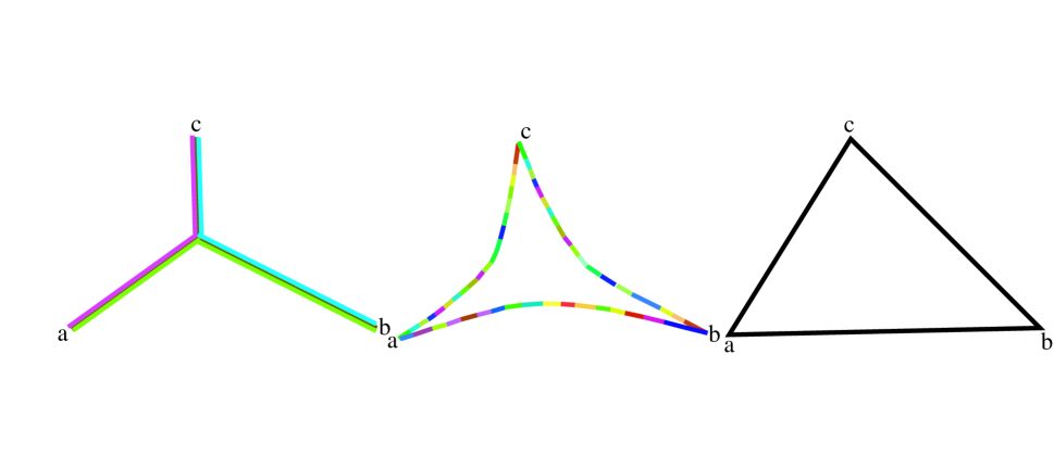
Figure 6. Three triangles illustrating non-positively curved spaces. The center one represents three points (trees) in treespace, a, b and c, with the geodesics running between them (notice the paths are made of sequences of segments that sit in the Euclidean cubes of the cube complex, but we can see an overall negative curvature, i.e. triangles are thin compared to the Euclidean comparison triangle on the right). The left triangle depicts the situation in which the space is so negatively curved as to be a tree.

This is illustrated by Figure 6, which shows three geodesic triangles in three different types of space. On the left, a $\delta$-hyperbolic metric space with $\delta$=0, is actually a tree.

$\delta$-hyperbolic metric space

1. Consider a geodesic triangle: 3 vertices connected by geodesic paths. It is $\delta$-thin if any point on any of the edges of the triangle is within distance $\delta$ from one of the other two sides.

2. A $\delta$-hyperbolic space is a geodesic metric space in which every geodesic triangle is $\delta$-thin.

As we can see in Figure 6, the ‘triangle in a tree’ on the left is represented by the three colored edges (made of two segments each) and has the property that each point from an edge, for instance a point on the pink edge $ac$ is within $\delta=0$ from the closest other edge, either the blue or the green are at distance $0$. The middle triangle has a $\delta=0.25$ (if we think the long side $d(a,b)$ is 1), and the right triangle has a $\delta=0.5$. Euclidean space actually does not have a bounded $\delta$, ($\delta=\infty$), as triangles can be chosen to be arbitrarily large.

The question raised by Figure 6 and that we will try to address is whether we can make the best approximate representation of many trees given their BHV distances by embedding the points in a Euclidean space using a modified MDS or whether it is better to place the trees in a tree, as we do in the last section of the paper. The question of choice between spatial and treelike representations is an old one and was clearly posed by Pruzansky, Tversky, and Carroll (1982) almost 30 years ago in the context of dissimilarities measured on psychological preferences. We introduce a more quantitative notion by computing the $\delta$-hyperbolicity of a set of distances between a finite set of points. The question of the quality of a treelike approximation is considered in section 4. In the next section we will show how to measure the quality of a Euclidean approximation.

3.2. Multidimensional Scaling and its application to tree comparisons

Psychometricians, ecologists and statisticians have long favored a method known as multidimensional scaling (MDS) to approximate general dissimilarities with Euclidean distances.

MDS is a statistical method developed around Schoenberg’s theorem that a symmetric matrix of positive entries with zeros on the diagonal is a distance matrix between $n$ points if and only if the matrix

$$-\frac{1}{2}HD^{2}H\mbox{ is positive semi-definite }$$

We will not provide the details of the algorithm, referring the reader to (Mardia, Kent, and Bibby, 1979, p.407) but offer the following summary: Given an $n\times n$ matrix of interpoint distances, one can solve for points in Euclidean space approximating these distances by:

1. Double centering the interpoint distance squared matrix: $S=-\frac{1}{2}HD^{2}H$.

2. Diagonalizing $S$: $S=U\Lambda U^{T}$.

3. Extracting $\tilde{X}$: $\tilde{X}=U\Lambda^{1/2}$.

We use the standard implementation provided in the stats package of R Ihaka and Gentleman (1996) by the function cmdscale. We can estimate the quality of the approximation of the distances $d$ using the Euclidean approximation by computing an index such as

$$\sum_{i<j}(d_{ij}-\delta_{ij})^{2}.$$

This index will be zero if the data come from a $k$ dimensional Euclidean space and we retain as $k$ dimensions in our multidimensional scaling.

As we will see later, since we know our tree points lie on a curved space where local distances are nearly Euclidean but points further apart are not, we will sometimes be better off making modifications to the distances before applying MDS.

3.3. MDS of Bootstrapped Trees

One approach to inference for hierarchical clustering and phylogenetic trees is to simply apply a nonparametric resampling bootstrap to the data and re-estimate the trees. This gives an idea of the overall variability of the data under the assumption that the unknown distribution of the distances $d(\tau,\hat{\tau})$ can be well approximated by that of $d(\hat{\tau},\hat{\tau}^{*})$ , where $\hat{\tau}^{*}$ denotes the bootstrapped estimates of the tree.

Here we apply this idea in conjunction with a MDS plot, using a bootstrap of the the Laurasiatherian DNA data from the package phangorn (Schliep, 2009). The original estimate is shown in Figure 7.

Figure 7. Tree Estimate from aligned DNA sequences of length 3179.

Tree type	count
1	6
2	12
3	2
4	37
5	4
6	1
7	9
8	21
9	5
10	3
11	5
12	1
13	7
14	1
15	4
16	8
17	2
18	2

Tree type	count
19	1
20	3
21	4
22	10
23	6
24	2
25	5
26	14
27	3
28	1
29	4
30	1
31	1
32	1
33	3
34	5
35	1
36	2

Tree type	count
37	2
38	1
39	1
40	2
41	2
42	1
43	5
44	1
45	2
46	3
47	3
48	2
49	2
50	2
51	1
52	1
53	1
54	1

Tree type	count
55	1
56	2
57	1
58	2
59	1
60	1
61	1
62	2
63	1
64	1
65	1
66	1
67	1
68	1
69	1
70	1
71	1
72	1

Table 1. Binned Bootstrapped Trees. Of the 250 bootstrapped trees, there is a majority of type 4.

Table 1 shows that the 250 trees are of 72 different types or branching orders. An MDS plot of the first two principal coordinates using the BHV distance is presented in Figure 8.

If we compute a simple Shannon type diversity index, we get the impression that the trees are very diverse (SW=$-\sum p_{i}\log(p_{i})-\frac{S-1}{2*N}$=-sum(freq*log(freq))-(71/502)=3.5).

In fact the trees as represented in Figure 8 are quite grouped.

It is an interesting question how to study the variability of trees, whether using a diversity index or an ‘inertia’ type approach using such sums of squares of distances. The original estimate projects at the center of the scatterplot, leading us to believe that the estimate is unbiased.

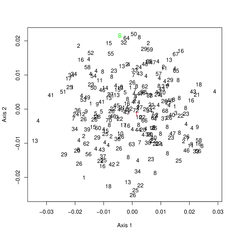
Figure 8. First MDS plane representing 250 bootstraps. The tree topologies were numbered from 1 (the original tree) to 72. We have plotted the orginal bootstrap estimate in red as 1, and the star tree with the pendant edge lengths matching those of the original tree represented by the letter S in green.

As an additional element we have projected the star tree “S” (chosen with the lengths of the pendant edges closest to the original tree) to see whether it is in a small neighborhood, or credibility region of the bootstrapped trees. This is analogous to seeing if $0$ is in a confidence interval of differences between two random variables. If the star tree seems to be in a confidence region with a high probability coverage then we may conclude that the data are not really treelike. In Figure 8, $S$ appears to be on the outer convex hull of the projected points; we can conclude that the probability that the star tree belongs to the confidence region is low. See Holmes (2005) for details on the idea of using convex hulls to make confidence statements of this type.

Looking at Figure 8 we can see that trees of the same topology are not necessarily closer to the original tree if we use the BHV with no modifications. In some cases we may want to give an extra weight to crossing orthants. We give examples of such modifications of the distance in the Chakerian and Holmes (2010) vignette.

3.4. Empirical Evidence of Mixing on the Bethe Lattice

Erdős et al. (1999) have shown that the tree shape that requires the longest sequence length for inferring the root as accurately as possible is the balanced tree. Mossel (2004) recognized this tree shape as the Bethe Lattice, known in statistical mechanics, and used this fact to give bounds on the sequence lengths necessary to rebuild the tree accurately with a given probability. For this shape, Mossel (2004) showed that if mutation rates are high it is impossible to reconstruct ancestral data at the root and the topology of large phylogenetic trees from a number of characters smaller than a low-degree polynomial in the number of leaves.

Figure 9. Balanced tree on 64 leaves, known as the Bethe Lattice, we have added an outgroup to fix the root.

3.5. Seeing the Mutation Rate Gradient on Bethe Trees

We generated 9 sets of trees with mutation rates set from $\alpha=0.01$ to $\alpha=0.09$ and we generated the data according to the Bethe lattice tree.
Here are the results in the first plane of the MDS:

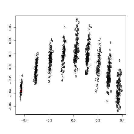
Figure 10. The first two axes of the MDS of 901 trees with mutation rates varying from $\alpha=0.01$ to $\alpha=0.09$ (as labeled)

This shows that multidimensional scaling can be useful for comparing trees which have differing mutation rates. The arch shape for the overall trend is a classical instance of the horseshoe phenomenon Diaconis et al. (2007). It is an open question as to whether such a plot could be useful in the inverse problem of trying to estimate the relevant mutation rate for a data set, given the bootstrapped trees generated using the parametric bootstrap with differing mutation rates.

3.6. Finding inconsistent characters with high leverage

In regression it is often useful to find observations with high leverage. High leverage in regression can be detected by seeing a large jump in the fitted model after the point is taken out. In the phylogenetic context, if a character or a set of contiguous characters are taken out of the data and the tree changes, this can be an indication of recombination or horizontal transfer events. In previous work de Oliveira Martins et al. (2008) use the the minimum number of subtree prune-and-regraft (SPR) operations required to resolve inconsistencies between two trees to detect recombination events along DNA sequences in HIV.

Our approach is simpler since we will not use a Bayesian posterior, just the distance between the original tree and the tree without the character/segment.

Figure  1 in the first example show the MDS plot built from distances between each of the cross-validation data sets built by excluding a single gene and recomputing the hierarchical clustering tree and then computing the BHV distance between trees. Each cross validated tree is labeled by the gene that is excluded. Table 4 in the supplementary material shows the distances between the cross-validated trees and the original tree. If we consider the distances to the original tree in the first row as shown in 2, we can see that they are basically bimodal, a group around at a distance of about 17 from the original tree and a group of values around 20 but the plot in Figure 1 tells a richer story since it shows how the genes can be organized into three clusters according to the effect they have on the overall hierarchical clustering tree. In some sense, this gives us a picture of the leverage of each gene.

	Ori.	SNN	AF.	PLAG.	DHR.	PASK	PDE.	CAC.	LRR.	F2R	CX3.	MAD.	PPP.	KIF22	MGC.	BCR	IFI.	TRIM.
Ori.	0	22	17	23	20	17	21	16	16	16	16	22	22	16	18	17	21	17

Table 2. Rounded distances between the cross-validated trees and the original tree

4. Tree of trees

A tree is a complete CAT(0) space (Gromov, 1987). Since Billera et al. (2001) showed that the space of trees is also a CAT(0) space (as shown in Figure  6, this can be visualized by considering that triangles are thin compared to Euclidean ones), we might guess a tree of trees would be a satisfactory representation of a sample from the Bayesian posterior or a bootstrap resampling distribution of trees.

We know that given a distance matrix we can give a treelike representation of the points with these distances by building a tree if the distances obey Buneman’s four point condition (Buneman, 1974).

Buneman’s four point condition

For any four points $(u,v,w,x):$
The two largest of the three sums:$d(u,v)+d(w,x),d(u,w)+d(v,x),d(u,x)+d(v,w)$ are equal.

We can see Gromov’s definition the hyperbolicity constant $\delta$ (Gromov, 1987) as a relaxation of the above four-point condition:

Gromov’s hyperbolicity constant

For any four points u,v,w,x, the two larger of the three sums $d(u,v)+d(w,x),d(u,w)+d(v,x),d(u,x)+d(v,w)$ differ by at most 2$\delta$.

We propose using the smallest $\delta$ that works as a numeric criteria to quantify how treelike a set of finite points with a geodesic metric is.

Conside the bootstrap example in section 3.3, where we have $B\times B$ matrix of distances. We can use the following to compute $\delta$:

Algorithm to compute the $\delta$-hyperbolicity

For all sets of 4 points among $B$, call them (i,j,k,l)
(of which there are $R=\frac{B(B-1)(B-3)(B-4)}{24}$).
For ( r from 1 to R) do (1)(2)(3) below:

1. Compute $A_{1}=d_{ij}+d_{kl},\qquad A_{2}=d_{ik}+d_{jl}\qquad A_{3}=d_{il}+d_{jk}.$

2. Sort $A_{1},A_{2},A_{3}\mbox{ giving }(A_{(1)},A_{(2)},A_{(3)})\mbox{ in decreasing order.}$

3. $\mbox{Take }E(r)_{=}(A_{(1)}-A_{(2)})$

$\mbox{Take }\delta=\frac{1}{2}\max_{r}E(r)$

The algorithm is implemented in the distory package. It takes about a minute to compute the $\delta$ -hyperbolicity of a $500\times 500$ distance matrix. In order to calibrate how small delta becomes both on uniformly distributed data in Euclidean space and on a finite treelike data set generated from balanced Bethe trees, we ran simulations where we generated points from known trees and then computed various distances between them.

Data	Distribution	Distance	Max (sd)	Mean(sd)	$\delta$ (sd)	$\delta$/Max (sd)
500 points	Uniform	Manhattan	13.8 (0.33)	8.33 (0.04)	7.03 (0.26)	0.51 (0.02)
500 points	Uniform	Euclidean	3.04 (0.06)	2.03 (0.009)	1.38 (0.05)	0.45 (0.02)
512 points	MVNormal	Manhattan	49.14 (1.59)	28.22 (0.20)	21.45 (0.79)	0.44 (0.02)
512 points	MVNormal	Euclidean	11.66 (0.41)	7.00 (0.05)	4.82 (0.17)	0.41 (0.02)
512 points	Bethe Tree	JC69	0.223 (0.008)	0.16 (0.003)	0.017 (0.001)	0.076 (0.0043)
512 points	Bethe Tree	Raw	0.19 (0.006)	0.14 (0.002)	0.013 (0.001)	0.069 (0.004)
500 trees	rtree	BHV	8.03	6.46	0.68	0.085
30 leaves	uniform splits
500 trees	rtree	BHV	8.94	7.53	0.60	0.067
40 leaves	uniform splits
500 trees	rtree	BHV	9.91	8.52	0.63	0.064
50 leaves	uniform splits
500 trees	rtree	BHV	10.45	9.32	0.59	0.056
60 leaves	uniform splits
500 trees	rtree	BHV	11.50	10.09	0.59	0.051
70 leaves	uniform splits

Table 3. Different values of $\delta$ and the ratio $\delta$/max(d) for points generated both in bounded Euclidean space and for points generated from trees. In the top half of the table, each value was estimated from 100 simulations, in the Euclidean case the distances were computed from points generated in 25 dimensions. In the lower half of the table the values were generated by randomly generated trees of a given size, 30,40,50,60 and 70 leaves and looking at the maximum and $\delta$ values for this sample of 500 trees. We can see that the sets of randomly generated trees have a much lower $\delta$-hyperbolicity and little variation with the number of leaves in the tree.

In particular, we used the $\delta/max$ statistic in the case of the bootstrapped trees represented by the MDS plot in the resulting ratio was $0.47$. This indicates given, the calibration experiments in the above table, that point configuration would be well approximated by a Euclidean MDS. The $\delta/max$ statistic is a rough approximation for scaling each triangle considered by its diameter; two other approximations, scaling by the perimeter and scaling by the max of the sums $A_{(1)}$ are implemented in the R package.

We note here that recently, theoretical computer scientists have used the geometry of graphs for algorithmic purposes following the breakthrough paper by Linial et al. (1995). The computation of $\delta$-hyperbolicity provided here could also be used in this context. There is also a healthy literature connected to the subject of metric graphs that includes other applications of $\delta$ hyperbolicity, for a comprehensive review see Bandelt and Chepoi (2008).

4.1. Mixture Detection

A particularly interesting application of this idea is in the detection of mixtures of the evolutionary processes underlying aligned sequences. Mixtures pose problems when using MCMC methods in the Bayesian estimation context (Mossel and Vigoda, 2005). These authors note that MCMC methods in particular those used to compute Bayesian posterior distributions on trees can be misleading when the data are generated from a mixture of trees, because in the case of a ‘well-balanced’ mixture the algorithms are not guaranteed to converge. They recommend separating the sequences according to coherent evolutionary processes. But this means the first step in the analyses of aligned sequences should be the detection of the mixture and proposals for separating the data at certain positions.

Suppose the data come from the mixture of several different trees; we will see how the bootstrap and the various distances and representations can detect these situations.

Our procedure uses the bootstrap or a Bayesian posterior distribution. Suppose we have $\tau_{1},\tau_{2},\ldots,\tau_{K}$ $K$ trees generated from one original alignment either by bootstrapping the original data or by using a MCMC method for generating from the Bayesian posterior. We use the distance between trees to make a hierarchical clustering tree using single linkage to provide a picture of the relationships between the trees.

In this simulated example we generate two sets of data of length $1,000$ from the two different trees. We concatenate the data into one data set on which the standard phylogenetic estimation procedures are run. This provides the estimated tree for the data. We then generate 250 bootstrap resamples from the combined data, and compute the distances between the 250 trees from each of the bootstrap resamples, using these to make a hierarchical clustering single linkage from this distance matrix.

Figure 11. Hierarchical clustering of 250 trees resulting from a nonparametric bootstrap of the data generated by the double data set $\mathcal{X}_{12}$

4.2. Variability of Trees from a Bayesian Posterior Distribution

After running MCMC Bayesian sampling from the posterior such as that available in MrBayesHuelsenbeck and Ronquist (2001) we obtain several sets of trees from different runs of the chain. In order to evaluate these picks, we took 250 random picks from the two runs combined, with the first 200,000 trees from each run discarded. Each MCMC was run 1,000,000 times on the same subset of the Laurasiatherian data available in the phangorn package (Schliep, 2009). We computed the $\delta/max$ statistic for the distance matrix between all 250 trees and obtained a value of $0.57$ indicating that the trees could be well approximated by a Euclidean representation.

The standard MDS plot is shown in Figure 12. We see that the scatterplot is bimodal, but this cannot be explained either by the runs, the trees sampled during the first run are given as ’*’ whereas the trees from the second runs are the ”#” character.

There were 5 different branching patterns in all, from run one there $(42,2,15,47,3)$ of each of the five categories of trees and $(52,0,27,57,6)$ in the second run (note both tuples represent counts of the same 5 topologies). We have colored each of these with one of five colors.

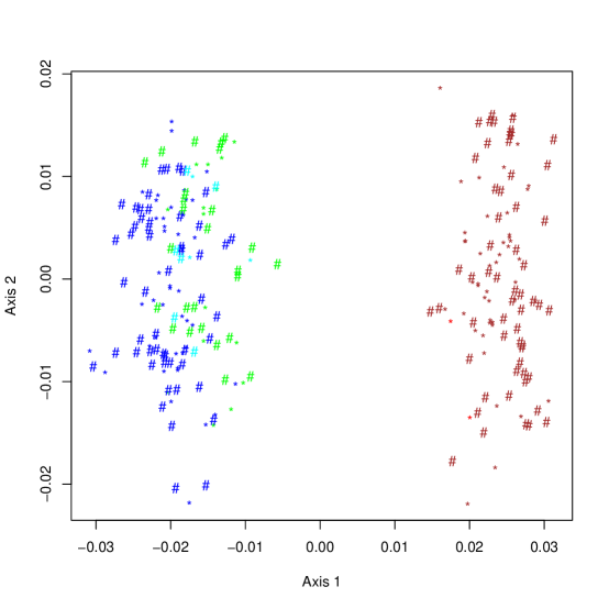
Figure 12. First plane of MDS plot (41%) of the trees sampled from the Bayesian posterior. The cloud on the right contains trees all from the same branching pattern (color indicates branching pattern), with an equal number of picks from the first run as from the second.

4.3. Kernel Multidimensional Scaling

It often makes sense to transform the distances so that the graphical representation focuses on correctly representing differences between similar points and doesn’t try to make a good representation of the distances between points which are far apart. This has been shown to be particularly effective when the original points lie on a postiviely curved manifold as for instance in (Tenenbaum et al., 2000; Roweis and Saul, 2000). However it can also be useful in the context of trees where the very local distances are Euclidean and the negative curvature only appears as points get further apart. Thus we will use the exponential kernel that takes the distance between trees $d(T_{1},T_{2})$ and compute a new dissimilarity measure between trees as $\delta(T_{1},T_{2})=1-exp(-\lambda d(T_{1},T_{2}))$ Then $\delta(T_{1},T_{2})\approx\lambda d(T_{1},T_{2})$ for $d(T_{1},T_{2})\ll 1$ and $\delta(T_{1},T_{2})\approx 1$ if $d(T_{1},T_{2})$ is large, so it will not be sensitive to noise around relatively large values of $d(T_{1},T_{2})$.

This kernel has the effect of representing carefully relations between close trees and thus is very useful for exploring local neighborhoods of treespace.

4.4. Learning the Right Distances

There are reasons to think that these distances are not giving us all the information we are looking for. If this is the case, we could ask the inverse question, given a set of trees and a distance which seems to be a meaningful representation of similarities, we can ask the inverse question of how to combine the topological information about the tree into the ‘right distance’. For instance if we are told that set $S_{1}$ of trees should be similar and different from another set $S_{2}$, we can make a parametric model that weights partitions on the tree so as to be concordant with this notion. There have been similar approaches to problems in text analysis solved by what is often called “metric learning”, for a recent illuminating example see Lebanon (2006).

In multivariate analysis it is often important to account for differing levels of variability in the data by rescaling variables. In the context of phylogenetic trees, for instance for the case where the contemporary DNA sequences are used to build trees that go far back in the past, it seems natural to ask if it wouldn’t be better to put differential weights on the branches of the tree to compensate for the higher uncertainty with which we can only infer what is happening high up in the tree(Mossel, 2004). In the same way we rescale variables so they have the same variance before doing a multivariate analysis, we would divide the edges in the tree closer to the root with larger numbers corresponding to the larger uncertainty, so that large differences higher in the tree would be downweighted as we are not sure of them. Examples of this differential weighting can be found in the vignette that accompanies the package distory (Chakerian and Holmes, 2010).

5. Using the path between two trees to find boundaries

It can be useful to explore both the neighborhood of a given tree and the datasets which are borderline in the sense that small perturbations induce a change in the tree topology.

5.1. Paths between different tree topologies

How close our estimate is to being borderline, in a particular sense of closeness, will inform us on the stability of our estimate. This can be done by creating small perturbations of the original data by bootstrapping. Looking at the set of bootstrapped trees, we can study the changes possible from small perturbations induced on the tree, both as changes in the topology and as quantitative measurements of distance. If all the bootstrap resamples give the same tree, then we are sure that the estimate we have is not ”borderline,” that is, the topology of the estimate is the same as that of the true tree.

However if the bootstrap resamples give many different trees it may be that the original data are not very treelike and the inferred tree has many competing neighbors.

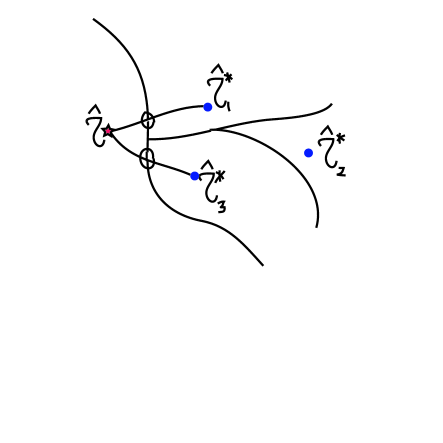
Figure 13. Example of three bootstrap trees (with stars) and the tree estimated from the original data. We see that trees $\hat{\tau}^{*}_{1}$ and $\hat{\tau}^{*}_{3}$ share a common boundary with the original estimate $\hat{\tau}$. We are particularly interested in borderline trees, ie trees at the intersection between the paths between trees and the boundaries between regions defined by each topology.

It can be interesting to know whether all the alternative bootstrap trees are the same, as happens in the case of an underlying mixture of trees, or whether there are a large number of competing trees, this will incline us more towards concluding that the data are far from treelike. In fact, if the star tree with all edges equal to zero is close to the original tree then the number of alternatives will be exponentially large (Holmes, 2005). If $r$ contiguous edges of the tree are small, there will still be $(2r-3)!!=(2r-3)\times(2r-5)\times..3\times 1$ trees in its close neighborhood.

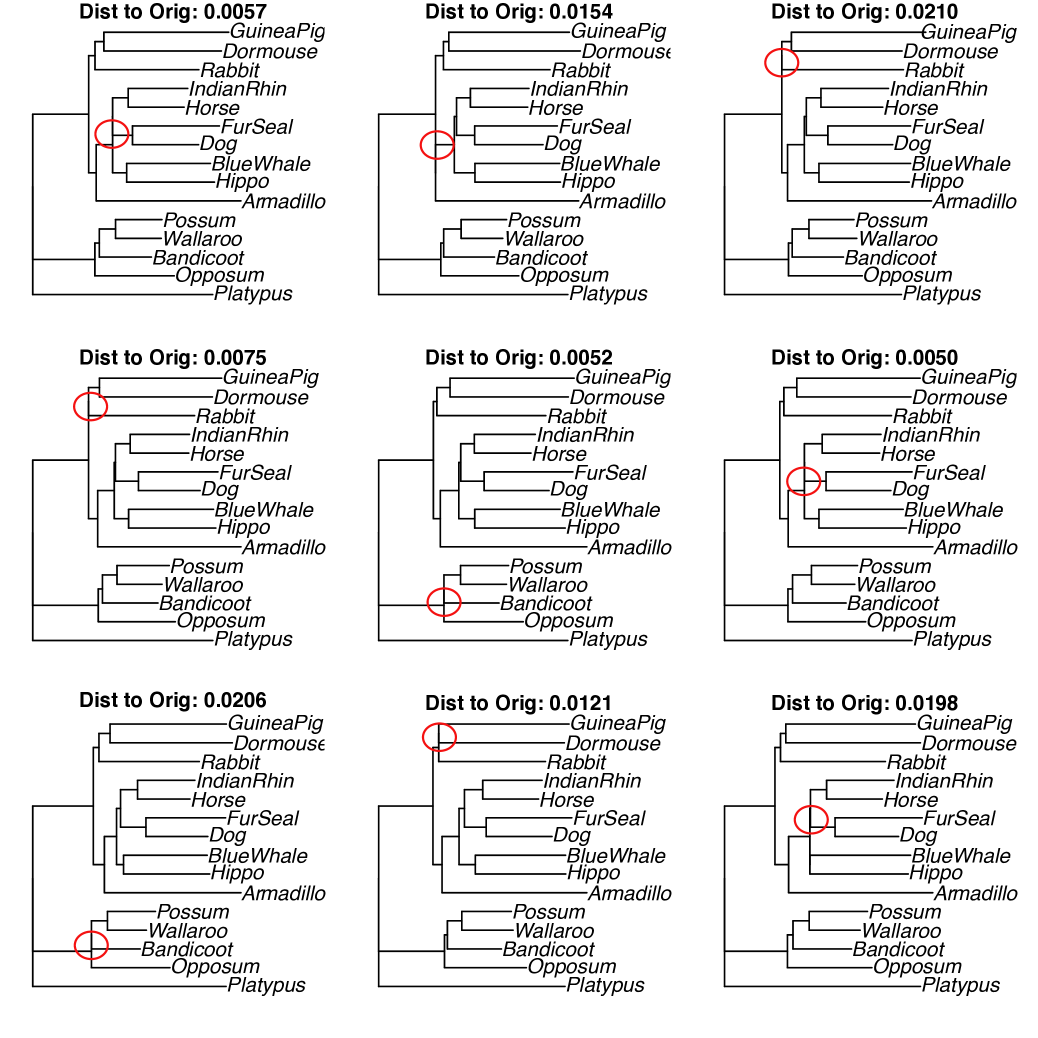
Figure 14. All 9 neighboring trees from the bootstrap of the Laura12 tree.

In the case of the bootstrap analysis whose binned topologies are presented in Table 1 we found that there are actually 9 trees in the bootstrap resample of that are borderline neighbors to the original tree, these neighbors and their respective BHV distances to the original tree are presented in the supplementary data (Figure  14). We see that there are thus many ‘small edges’ in this particular tree estimate, and the original estimated tree shares boundaries with $9$ competing orthants.

5.2. Finding Borderline Data with MCMC

After we estimate a tree based on a specific set of DNA sequences, we may be interested in seeing which particular changes to the original sequences may lead to alternative topologies.

We can use Markov Chain Monte Carlo methods to help with this: given a target tree with the topology of interest, we try to find a configuration of weights for the columns from the original sequences such that the tree estimated from data sampled from those weights is as close to the target tree (on the boundary) as possible.

We start with the original sequences, such that every position in the sequences occurs once; we then draw proposals of increasing the count of one position by one and decreasing the count of another by one, to maintain the same number of total base pairs in the dataset (intuitively, we write over the DNA at one position with that from another position in such a way that the DNA at the position we wrote over can still be used again). A tree is estimated with the proposed change, and the proposal is accepted or rejected based on the ratio of the old distance to the new distance (if the new distance is smaller, the ratio is greater than 1, so the proposal is accepted automatically; if the new distance is greater, with some probability the proposal is accepted anyway to allow the MCMC to get out of local minima). A simulated annealing scheme (Kirkpatrick, 1984) introduces a temperature which is used to help with location of a closest approximating set of positions, which are then reported along with the resulting tree and the final distance. This algorithm has been implemented in R (Ihaka and Gentleman, 1996) and is also available in the distory (Chakerian and Holmes, 2010) package.

6. Conclusions : More questions than answers.

We have combined the problems of evaluating phylogenetic trees and hierarchical clustering displays in a common mathematical framework. By embedding rooted binary trees in a metric space associated to the BHV distance, we can capitalize on statistical methods such as MDS to solve some of the difficulties in evaluating distributions of trees as output by Bayesian posterior sampling or bootstrap methods.

We show through examples that a distance between trees can provide valuable information about the variability of tree estimates and a substitute notion of multivariate spread. However, many questions remain unanswered.

At a fundamental level, what are realistic probability measures on treespace and how they should be used to provide useful priors and a theoretical notions of variance and more general moments on the space?

More generally, we face the issue of a practical way of quantifying variability of points. This question in tree space has a resemblance with phylogenetic diversity (Faith, 1992). Trees could be considered leaves on a tree of trees, and thus a more nuanced measure of diversity than a simple Shannon type index is available.

Here we propose Gromov’s $\delta$-hyperbolicity constant as a useful statistic for evaluating if the points in treespace were better approximated by a tree of trees or a Euclidean approximation. However, many open questions remain around this topic. We have only touched briefly on the question of the correct scaling of the $\delta$ statistic; our choice was to take the maximum distance between two points, but other choices can be argued, recently Jonckheere et al. (2008) choose a more ‘exact’ normalization that comes with high computational price, their suggestion is to compute the diameter of all the geodesic triangles (two simpler methods, using the perimeter and max of the sums, may be good approximations as well and are available in the distory (Chakerian and Holmes, 2010) package).

Nothing is known about the distributional theory of Gromov’s $\delta$ statistic. Its dependence on the underlying dimension and sparsity of the data is obvious, but there is much more work to be done before valid inferential methods become available for evaluating both the local and the global curvature of a finite set of points.

Finally we have shown how the BHV distance can be used to evaluate the distance to the boundary tree closest to it and to some of the data sets that could have given such a tree. More work needs to be done to provide accurate leverage statistics for trees.

Supplementary Data

	Ori.	SNN	AF.	PLAG.	DHR.	PASK	PDE.	CAC.	LRR.	F2R	CX3.	MAD.	PPP.	KIF22	MGC.	BCR	IFI.	TRIM.
Original	0	22	17	23	20	17	21	16	16	16	16	22	22	16	18	17	21	17
SNN	22	0	33	34	32	34	32	29	32	30	33	31	34	33	33	33	33	33
AF5q31	17	33	0	34	31	17	31	18	16	17	15	31	34	15	16	12	32	15
PLAG1	23	34	34	0	33	29	14	32	31	32	30	18	10	31	32	34	31	33
DHRS3	20	32	31	33	0	31	30	27	29	26	29	31	33	28	32	29	25	31
PASK	17	34	17	29	31	0	30	18	12	17	9	33	30	12	13	16	28	14
PDE9A	21	32	31	14	30	30	0	31	29	31	30	12	11	29	31	33	30	33
CACNB3	16	29	18	32	27	18	31	0	14	9	17	30	32	17	18	14	30	18
LRRC5	16	32	16	31	29	12	29	14	0	15	10	32	31	9	11	14	27	16
F2R	16	30	17	32	26	17	31	9	15	0	16	31	33	15	18	12	31	17
CX3CR1	16	33	15	30	29	9	30	17	10	16	0	33	31	8	11	12	27	16
MAD-3	22	31	31	18	31	33	12	30	32	31	33	0	16	32	34	32	33	32
PPP2R2B	22	34	34	10	33	30	11	32	31	33	31	16	0	32	32	35	32	33
KIF22	16	33	15	31	28	12	29	17	9	15	8	32	32	0	11	14	27	17
MGC4170	18	33	16	32	32	13	31	18	11	18	11	34	32	11	0	16	31	18
BCR	17	33	12	34	29	16	33	14	14	12	12	32	35	14	16	0	31	14
IFI16	21	33	32	31	25	28	30	30	27	31	27	33	32	27	31	31	0	32
TRIM26	17	33	15	33	31	14	33	18	16	17	16	32	33	17	18	14	32	0

Table 4. Rounded distances between cross validated hierarchical clustering trees and the one computed using all the genes.

References

- Bandelt and Chepoi (2008) H.J. Bandelt and V. Chepoi. Metric graph theory and geometry: a survey. In Surveys on discrete and computational geometry, volume 453 of Contemp. Math., pages 49–86. Amer. Math. Soc., Providence, RI, 2008.
- Billera et al. (2001) L. Billera, S. Holmes, and K. Vogtmann. The geometry of tree space. Adv. Appl. Maths, 771–801, 2001.
- Breiman et al. (1984) L. Breiman, J. H. Friedman, R. A. Olshen, and C. J. Stone. Classification and Regression Trees. Wadsworth, 1984.
- Bridson and Haefliger (1999) M.R. Bridson and A. Haefliger. Metric spaces of non-positive curvature. Grundlehren der math Wiss. Springer Verlag, 1999.
- Buneman (1974) P. Buneman. A note on metric properties of trees. Journal of Combinatorial Theory, Jan 1974.
- Chakerian and Holmes (2010) J. Chakerian and S. Holmes. distory:Distances between trees, 2010. URL http://cran.r-project.org/web/packages/distory/index.html.
- de Oliveira Martins et al. (2008) L. de Oliveira Martins, E. Leal, and H. Kishino. Phylogenetic detection of recombination with a bayesian prior on the distance between trees. PLoS ONE, 3(7):e2651, Jan 2008. doi: 10.1371/journal.pone.0002651.
- Diaconis et al. (2007) P. Diaconis, S. Goel, and S. Holmes. Horseshoes in multidimensional scaling and kernel methods. Annals of Applied Statistics, 2007.
- Drummond and Rambaut (2007) A J Drummond and A Rambaut. Beast: Bayesian evolutionary analysis by sampling trees. BMC Evol Biol, 7:214, Jan 2007. doi: 10.1186/1471-2148-7-214. URL http://www.biomedcentral.com/1471-2148/7/214.
- Efron (1979) B. Efron. Bootstrap methods: Another look at the jackknife. The Annals of Statistics, 7:1–26, 1979.
- Efron et al. (1996) B. Efron, E. Halloran, and Susan P. Holmes. Bootstrap confidence levels for phylogenetic trees. Proc. Natl. Acad. Sci. USA, 93:13429–34, 1996. ISSN 1091-6490.
- Erdős et al. (1999) PL Erdős, MA Steel, László A. Székely, and TJ Warnow. A few logs suffice to build (almost) all trees. I. Random Structures Algorithms, 14(2):153–184, 1999. ISSN 1042-9832.
- Faith (1992) D. Faith. Conservation evaluation and phylogenetic diversity. Biological Conservation, Jan 1992.
- Felsenstein (1983) J. Felsenstein. Statistical inference of phylogenies (with discussion). Journal Royal Statistical Society A, 146:246–272, 1983.
- Felsenstein (2004) J. Felsenstein. Inferring Phylogenies. Sinauer, Boston, 2004.
- Foulds and Graham (1982) L. R. Foulds and R. L. Graham. The Steiner problem in phylogeny is NP-complete. Adv. in Appl. Math., 3(1):43–49, 1982. ISSN 0196-8858.
- Fowlkes and Mallows (1983) E Fowlkes and C Mallows. A method for comparing two hierarchical clusterings. Journal of the American Statistical Association, Jan 1983. URL http://www.jstor.org/stable/2288117.
- Gromov (1987) M. Gromov. Hyperbolic groups. In Essays in group theory, pages 75–263. Springer, New York, 1987.
- Guindon and Gascuel (2003) S. Guindon and O. Gascuel. A simple, fast, and accurate algorithm to estimate large phylogenies by maximum likelihood. Systematic Biology, 52:696–704, 2003.
- Hartigan (1967) J Hartigan. Representation of similarity matrices by trees. Journal of the American Statistical Association, Jan 1967. URL http://www.jstor.org/stable/2283766.
- Holmes (2003) S. Holmes. Bootstrapping phylogenetic trees: theory and methods. Statist. Sci., 18(2):241–255, 2003. ISSN 0883-4237. Silver anniversary of the bootstrap.
- Holmes (1999) S. Holmes. Phylogenetic trees: an overview. In Statistics and Genetics(Minneapolis, MN, 1997), number 112, pages 81–118. Springer,IMA, New York, 1999.
- Holmes (2005) S. Holmes. Statistical approach to tests involving phylogenies. In Mathematics of Evolution and Phylogeny. Oxford University Press, Oxford,UK, 2005.
- Huelsenbeck and Ronquist (2001) J. Huelsenbeck and F. Ronquist. MrBayes:Bayesian inference of phylogenetic trees. Bioinformatics, 17:754–755, 2001.
- Ihaka and Gentleman (1996) R. Ihaka and R. Gentleman. R: A language for data analysis and graphics. Journal of Computational and Graphical Statistics, 5(3):299–314, 1996.
- Jonckheere et al. (2008) E. Jonckheere, P. Lohsoonthorn, and F. Bonahon. Scaled Gromov hyperbolic graphs. J. Graph Theory, 57(2):157–180, 2008.