Coherent Quantum-Noise Cancellation for Optomechanical Sensors

Abstract

Using a flowchart representation of quantum optomechanical dynamics, we design coherent quantum-noise-cancellation schemes that can eliminate the back-action noise induced by radiation pressure at all frequencies and thus overcome the standard quantum limit of force sensing. The proposed schemes can be regarded as novel examples of coherent feedforward quantum control.

Noise introduces error to communication or sensing because it is unknown to the observer and cannot be distinguished from the desired signal. If the noise can be measured separately, one can physically or computationally remove the noise. This is the principle of noise cancellation, a technique that has seen widespread commercial application, especially for acoustic-noise control hansen : noise-cancelling headphones, for example, work by recording the ambient noise and playing it back with opposite amplitude to interfere destructively with the noise reaching the inner ear.

Here we consider the application of noise cancellation to quantum systems. We focus on optomechanical force sensors, in which quantum radiation-pressure fluctuations on a moving mirror within an optical cavity can introduce excess noise, called the back-action noise, in addition to the shot noise at the cavity output. This leads to the standard quantum limit (SQL) on detecting a classical force on the mirror braginsky . Various methods of quantum-noise reduction have been proposed to overcome the SQL, including frequency-dependent squeezing of the input light unruh ; bondurant84 ; kimble ; unruh_exp ; khalili10 , variational measurement vyatchanin ; kimble ; khalili10 , introducing a Kerr medium inside the optical cavity bondurant86 , and the use of dual mechanical resonators briant ; briant_exp or an optical spring buonanno ; buonanno_exp to modify the mechanical response function. Several of these proposals have been implemented unruh_exp ; briant_exp ; buonanno_exp , though not in the quantum regime. All can be regarded as quantum-noise-cancellation (QNC) schemes, which utilize destructive interference to reduce or eliminate the effects of back action. With back action tamed, squeezing of the input light caves can be used to improve sensitivity further.

To facilitate understanding of the QNC concept and design of new QNC schemes, we introduce the use of flowcharts to depict the quantum dynamics. Using the flowcharts, we design a few novel QNC schemes that can eliminate back-action noise at all frequencies and should require less space than previous broadband QNC schemes. Although the effects of quantum radiation-pressure noise are only now becoming detectable verlot09 , the field of optomechanics has recently seen rapid progress marquardt . Back-action noise is expected to become a major issue in future optomechanical sensors. Combined with quantum filtering and smoothing tsang , QNC has the potential to improve significantly the performance of future force sensors beyond conventional quantum limits. In the context of quantum control control , QNC schemes can be regarded as examples of coherent feedforward quantum control, to be contrasted with measurement-based feedforward control lam and coherent feedback control james techniques.

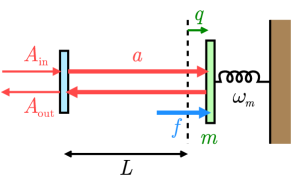
Figure 1: (Color online) Optomechanical force sensor.

Consider now a Fabry-Perot cavity with a moving mirror, as depicted in Fig. 1. The mirror is modeled optically as perfectly reflecting and mechanically as a harmonic oscillator with position operator $q(t)$, momentum operator $p(t)$, mass $m$, and resonant frequency $\omega_{m}$, subject to a force $f(t)$. The cavity is pumped with an input beam $A_{\rm in}(t)$, incident on the partially transmitting mirror on the left. We work in a rotating frame that removes the harmonic time dependence at the input beam’s carrier frequency $\omega_{0}$. All phases are referenced to the input field, which has constant (real) mean amplitude $\langle A_{\rm in}\rangle=\mathcal{A}_{\rm in}$. The intra-cavity field decays at rate $\gamma$ due to coupling through the partially transmitting mirror to the output beam $A_{\rm out}(t)$. The intra-cavity optical field $a(t)$ is assumed to be resonant at the carrier frequency $\omega_{0}$ when the mirror is displaced to its equilibrium position under the mean radiation pressure, at which point the round-trip length is $2L$. The mirror position $q(t)$ is defined relative to this equilibrium position. The force is estimated by continuous homodyne measurement of an appropriate quadrature of $A_{\rm out}$, labeled 2 in the following and usually the phase quadrature. The operators obey canonical commutation relations: $[q(t),p(t)]=i\hbar$, $[a(t),a^{\dagger}(t)]=1$, and $[A_{\rm in}(t),A_{\rm in}^{\dagger}(t^{\prime})]=\delta(t-t^{\prime})$.

One can generalize this basic setup to more elaborate configurations, e.g., more complicated optical and mechanical mode structures or detuned cavity excitation, which gives rise to an optical spring buonanno ; buonanno_exp . A major difference from a two-armed interferometer is that squeezed light must be input in the same beam as the mean field that powers the system. Nonetheless, this minimal setup already captures the salient features of cavity optomechanical systems.

The operator equations of motion are

$$\frac{dq}{dt} =\frac{p}{m}\;,\quad\frac{dp}{dt}=-m\omega_{m}^{2}q+\frac{\hbar\omega_{0}}{L}\left(a^{\dagger}a-\alpha^{2}\right)+f\;,$$

$$\frac{da}{dt} =-\gamma a+\frac{i\omega_{0}}{L}qa+\sqrt{2\gamma}A_{\rm in}\;,\quad A_{\rm out}=\sqrt{2\gamma}a-A_{\rm in}\;,$$ (1)

where $\alpha=\mathcal{A}_{\rm in}\sqrt{2/\gamma}$ is the mean cavity field ($\langle a^{\dagger}a\rangle=\alpha^{2}$). Removing mean fields and defining amplitude and phase quadrature operators for the fluctuations that remain, $A_{\rm in}=\mathcal{A}_{\rm in}+(\xi_{1}+i\xi_{2})/\sqrt{2}$, $A_{\rm out}=\mathcal{A}_{\rm in}+(\eta_{1}+i\eta_{2})/\sqrt{2}$, and $a=\alpha+(a_{1}+ia_{2})/\sqrt{2}$, one can linearize Eqs. (1) by neglecting quadratic terms and obtain a system of linear differential equations,

$$\frac{d\boldsymbol{x}}{dt}=\boldsymbol{F}\boldsymbol{x}+\boldsymbol{G}\boldsymbol{w}\;,\qquad\boldsymbol{y}=\boldsymbol{H}\boldsymbol{x}+\boldsymbol{J}\boldsymbol{w}\;.$$ (2)

Here the state variables $\boldsymbol{x}\equiv\begin{pmatrix}q&p&a_{1}&a_{2}\end{pmatrix}^{T}$, inputs $\boldsymbol{w}\equiv\begin{pmatrix}f&\xi_{1}&\xi_{2}\end{pmatrix}^{T}$, and output signals $\boldsymbol{y}\equiv\begin{pmatrix}\eta_{1}&\eta_{2}\end{pmatrix}^{T}$ are related by the matrices

$$\boldsymbol{F} \equiv\begin{pmatrix}0&1/m&0&0\\ -m\omega_{m}^{2}&0&\hbar\kappa&0\\ 0&0&-\gamma&0\\ \kappa&0&0&-\gamma\end{pmatrix}\;,\quad\boldsymbol{J}\equiv\begin{pmatrix}0&-1&0\\ 0&0&-1\end{pmatrix}\;,$$

$$\boldsymbol{G} \equiv\begin{pmatrix}0&0&0\\ 1&0&0\\ 0&\sqrt{2\gamma}&0\\ 0&0&\sqrt{2\gamma}\end{pmatrix}\;,\quad\boldsymbol{H}\equiv\begin{pmatrix}0&0&\sqrt{2\gamma}&0\\ 0&0&0&\sqrt{2\gamma}\end{pmatrix}\;,$$ (3)

where $\kappa\equiv\sqrt{2}\alpha\omega_{0}/L$ is an optomechanical coupling strength.

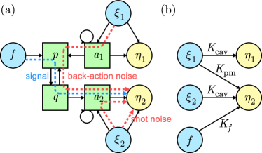
Figure 2: (Color online) (a) Flowchart representation of Eqs. (2) and (Coherent Quantum-Noise Cancellation for Optomechanical Sensors). (b) Simplified flowchart depicting only the input and output signals linked by transfer functions.

In control-system design, it is often illuminating to draw a block diagram to represent a system of differential equations franklin . Here we use a simpler depiction, which we call a flowchart, as shown in Fig. 2(a) for Eqs. (2) and (Coherent Quantum-Noise Cancellation for Optomechanical Sensors). Arrows point from a variable on the right-hand side of an equation of motion to a connected variable on the left-hand side. Since the system is linear, the output signals are sums of independent contributions from the inputs, so one can easily depict the flow of signal and noise from input to output. In Fig. 2(a), the dashed arrows depict contributions to the output quadrature $\eta_{2}$ from the signal $f$ and from the input amplitude and phase fluctuations, $\xi_{1}$ and $\xi_{2}$. The $\xi_{2}$ contribution is commonly known as shot noise, while the $\xi_{1}$ contribution is the back-action noise due to the Kerr-like ponderomotive coupling of the cavity amplitude quadrature $a_{1}$ to the phase quadrature $a_{2}$.

The solution for the state variables contains a transient solution, which decays exponentially and which can be ignored by pushing the initial time to $-\infty$. It is convenient to Fourier transform the remaining inhomogenous solution, writing $\boldsymbol{y}(\Omega)=\boldsymbol{K}(\Omega)\boldsymbol{w}(\Omega)$, where the overall transfer matrix is

$$\boldsymbol{K}(\Omega)=-\boldsymbol{H}(i\Omega\boldsymbol{I}+\boldsymbol{F})^{-1}\boldsymbol{G}+\boldsymbol{J}=\begin{pmatrix}0&K_{\rm cav}&0\\ K_{f}&K_{\textrm{pm}}&K_{\rm cav}\end{pmatrix}\;,$$ (4)

with $\boldsymbol{I}$ being the identity matrix. The cavity and ponderomotive transfer functions are

$$K_{\rm cav}(\Omega) =\frac{\gamma+i\Omega}{\gamma-i\Omega}\;, K_{\rm pm}(\Omega) =\frac{2\gamma\hbar\kappa^{2}/m}{(\omega_{m}^{2}-\Omega^{2})(\gamma-i\Omega)^{2}}\;,$$ (5)

and the signal transfer function is $K_{f}(\Omega)=K_{\rm pm}(\Omega)(\gamma-i\Omega)/\hbar\kappa\sqrt{2\gamma}$. A simplified flowchart that connects outputs to inputs by transfer functions is shown in Fig. 2(b).

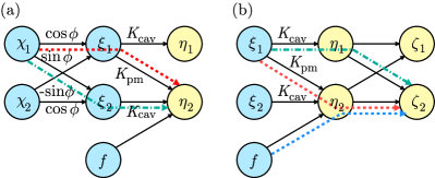
Figure 3: (Color online) (a) Frequency-dependent input squeezing. (b) Variational-measurement scheme.

Unruh’s proposal for frequency-dependent input squeezing unruh ; bondurant84 ; kimble ; unruh_exp ; khalili10 and Vyatchanin and Matsko’s variational-measurement scheme vyatchanin ; kimble ; khalili10 can be understood using flowcharts. First consider Unruh’s proposal, flowcharted in Fig. 3(a). The input beam, with quadratures $\chi_{1}$ and $\chi_{2}$, is processed through a passive system that rotates the quadratures by a frequency-dependent angle $\phi(\Omega)$, after which the beam is displaced by $\mathcal{A}_{\rm in}$ to produce the input field $A_{\rm in}$ to the optical cavity. The transfer functions from $\chi_{1}$ and $\chi_{2}$ to the output phase quadrature $\eta_{2}$ are $K_{\eta_{2}\chi_{1}}=K_{\textrm{pm}}\cos\phi+K_{\textrm{cav}}\sin\phi$ and $K_{\eta_{2}\chi_{2}}=-K_{\textrm{pm}}\sin\phi+K_{\textrm{cav}}\cos\phi$. The rotation is chosen to make the contribution from $\chi_{1}$ vanish, i.e., $K_{\eta_{2}\chi_{1}}=0$, by introducing destructively interfering paths from $\chi_{1}$ to $\eta_{2}$, as shown in Fig. 3(a). This requires $\tan\phi(\Omega)=-K_{\rm pm}(\Omega)/K_{\rm cav}(\Omega)$. Kimble et al. kimble devised a method for performing the dispersive rotation over a wide bandwidth by filtering the input beam through two detuned cavities. If the input to the filtering cavities is vacuum, the rotation has no effect on sensitivity; since $\chi_{2}$ is now entirely responsible for the output noise, however, it can be squeezed to improve the sensitivity to the shot-noise limit and beyond.

The variational-measurement scheme can be understood using the flowchart in Fig. 3(b). This scheme dispersively rotates the output light and measures the final output quadrature $\zeta_{2}$, which is a combination of the original output quadratures $\eta_{1}$ and $\eta_{2}$. This introduces an “anti-noise” path from $\xi_{1}$ to $\zeta_{2}$ via $\eta_{1}$, which can be used to cancel the original back-action noise path via $\eta_{2}$. Given the similarity of the flowcharts in Fig. 3, the required dispersive rotation is the same as that for Unruh’s proposal and can again be implemented using two detuned cavities. With back-action noise eliminated, the sensitivity is limited by shot noise and can be improved further by squeezing the input quadrature $\xi_{2}$ kimble .

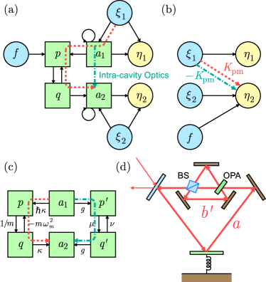
Figure 4: (Color online) (a) Back-action noise cancellation achieved by introducing an anti-noise path (green dash-dot arrow) from the intra-cavity amplitude quadrature $a_{1}$ to the phase quadrature $a_{2}$. (b) Simplified flowchart. (c) Detailed flowchart of the ponderomotive coupling and the intra-cavity matched squeezing. (d) An implementation of the matched squeezing scheme.

While the aforementioned schemes can be regarded as examples of coherent QNC, it is clear from Fig. 2 that a more direct way of cancelling the back-action noise is to introduce an anti-noise path from $a_{1}$ to $a_{2}$, as illustrated in Fig. 4. This calls for coherent processing of the intra-cavity field, using parametric interactions to undo the ponderomotive squeezing. The use of a Kerr medium bondurant86 , the dual-mechanical-resonator scheme briant ; briant_exp , and even an optical spring buonanno ; buonanno_exp can also be thought of as intra-cavity QNC schemes, but they cannot eliminate the back-action noise at all frequencies. To achieve broadband QNC, we introduce two auxiliary state variables, $q^{\prime}$ and $p^{\prime}$, which play the role of $q$ and $p$ in the anti-noise path, as shown in Fig. 4(c). Adjustable parameters $g$, $\mu$, and $\nu$, all with units of frequency, characterize the couplings in the anti-noise path. The anti-noise transfer function, indicated in Fig. 4(b) by the green dash-dot arrow, is $2\gamma\mu g^{2}/(-\mu\nu-\Omega^{2})(\gamma-i\Omega)^{2}=-K_{\textrm{pm}}$. We need $\mu\nu=-\omega_{m}^{2}$ and $\mu g^{2}=-\hbar\kappa^{2}/m$, thus requiring $\mu$ to be negative. This cannot be implemented by ponderomotive coupling to another mechanical oscillator unless its mass is negative.

The matched squeezing can nonetheless be achieved by coupling the intra-cavity field to an auxiliary field $b\equiv(q^{\prime}+ip^{\prime})/\sqrt{2}$. The required parameters are $\nu=-\mu=\omega_{m}$ and $g=\kappa\sqrt{\hbar/m\omega_{m}}=\alpha\omega_{0}\sqrt{2\hbar/m\omega_{m}}/L$, and the equations for $a$ and $b$ become

$$\frac{da}{dt} =-\gamma a+\frac{i\omega_{0}}{L}qa+\frac{ig}{2}(b+b^{\dagger})+\sqrt{2\gamma}A_{\rm in}\;,$$

$$\frac{db}{dt} =i\omega_{m}b+\frac{ig}{2}(a+a^{\dagger})-ig\alpha\;.$$ (6)

The auxiliary field should be inside another optical cavity, with resonant frequency $\omega_{0}-\omega_{m}$; it plays the role of a negative-energy mode in the anti-noise path. The constant driving term $-ig\alpha$, which removes the mean field from $b$, can be eliminated by redefining the auxiliary mode as $b^{\prime}=b-g\alpha/\omega_{m}$ and displacing the input field $A_{\textrm{in}}$, resulting in the following equations of motion:

$$\frac{da}{dt} =-\gamma a+\frac{i\omega_{0}}{L}qa+\frac{ig}{2}(b^{\prime}+b^{\prime\dagger})+\sqrt{2\gamma}A_{\rm in}^{\prime}\;,$$

$$\frac{db^{\prime}}{dt} =i\omega_{m}b^{\prime}+\frac{ig}{2}(a+a^{\dagger})\;,\quad A^{\prime}_{\rm in}=A_{\rm in}+i\mathcal{A}_{\rm in}\frac{g^{2}}{\gamma\omega_{m}}\;.$$ (7)

The coupling between $a$ and $b^{\prime}$ can then be realized using a beamsplitter (BS) and an optical parametric amplifier (OPA), as schematically shown in Fig. 4(d). With the back-action noise removed, only the shot noise from $\xi_{2}$ remains, and one can improve sensitivity further by increasing the optical power or by squeezing $\xi_{2}$.

In terms of the coupling constant $g$, the ponderomotive transfer function has the form

$$K_{\rm pm}(\Omega)=\frac{g^{2}}{\gamma\omega_{m}}\frac{\omega_{m}^{2}}{\omega_{m}^{2}-\Omega^{2}}\frac{2\gamma^{2}}{(\gamma-i\Omega)^{2}}\;,$$ (8)

so $|K_{\rm pm}(\Omega)|/|K_{\rm cav}(\Omega)|\sim g^{2}/\gamma\omega_{m}$ for frequencies away from the mechanical resonance; back action is thus important when $g\gtrsim\sqrt{\gamma\omega_{m}}$. The required single-pass idler gain of the OPA is thus $G\simeq(gL/c)^{2}\gtrsim\gamma\omega_{m}(L/c)^{2}\equiv G_{0}$. $G_{0}$ ranges from about $(2\pi\times 10~{}\textrm{Hz}\times 5~{}\textrm{km}/c)^{2}\simeq 10^{-6}$ for gravitational-wave detectors to $(2\pi\times 50~{}\textrm{MHz}\times 100~{}\mu\textrm{m}/c)^{2}\simeq 10^{-8}$ for microscale systems marquardt , so the required $G$ should be easily achievable with current OPA technology.

There is another potential problem: the number of photons in the auxiliary cavity in Fig. 4(d) is $\langle b^{\prime\dagger}b^{\prime}\rangle=g^{2}\alpha^{2}/\omega_{m}^{2}$, which becomes significantly higher than that in the primary cavity when $\omega_{m}$ is small, making the intra-cavity scheme problematic for applications that use high circulating power. This problem can be alleviated by using matched squeezing to modify the input or output optics. This requires the use of another double-cavity setup, similar to that in Fig. 4(d), but without the moving mirror, to pre-squeeze the input light going into the sensor cavity or post-squeeze the output light, as shown in Figs. 5(a) and (b). The flowcharts for these schemes, shown in Figs. 5(c) and (d), demonstrate broadband cancellation of back-action noise much like the intra-cavity scheme. If one is interested only in low frequencies $\Omega\ll\gamma$, the input/output matched squeezing can be implemented using smaller cavities with a larger decay rate $\gamma$ and a larger coupling constant $g$, with $g^{2}/\gamma$ held constant.

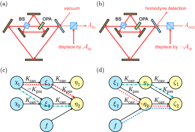
Figure 5: (Color online) Implementations of the (a) input and (b) output matched squeezing schemes and the associated flowcharts (c) and (d). For a two-armed interferometer, one only needs to squeeze the dark input or output port and does not need to perform the displacement.

We have assumed an ideal system, neglecting intrinsic mechanical and optical losses, to illustrate the essential features of QNC. Such assumptions are unrealistic in practice. To assess QNC schemes, it will be important to take into account the fluctuations associated with dissipation, such as the thermal noise associated with mechanical damping. The design and performance of QNC in the presence of realistic dissipation and noise deserve further investigation.

We acknowledge discussions with T. Kippenberg and S. Waldman. This work was supported in part by NSF Grant Nos. PHY-0903953 and PHY-0653596 and ONR Grant No. N00014-07-1-0304.

References

- (1) C. H. Hansen, Understanding Active Noise Cancellation (Taylor & Francis, London, 2001).
- (2) V. B. Braginsky and F. Ya. Khalili, Quantum Measurement (Cambridge University Press, Cambridge, 1992).
- (3) W. G. Unruh, in Quantum Optics, Experimental Gravitation, and Measurement Theory, edited by P. Meystre and M. O. Scully (Plenum, New York, 1982), p. 647.
- (4) R. S. Bondurant and J. H. Shapiro, Phys. Rev. D30, 2548 (1984); M. T. Jaekel and S. Reynaud, Europhys. Lett. 13, 301 (1990); A. Luis and L. L. Sánchez-Soto, Phys. Rev. A45, 8228 (1992).
- (5) H. J. Kimble et al., Phys. Rev. D65, 022002 (2001).
- (6) C. M. Mow-Lowry et al., Phys. Rev. Lett. 92, 161102 (2004).
- (7) F. Ya. Khalili, e-print arXiv:1003.2859, and references therein.
- (8) S. P. Vyatchanin and A. B. Matsko, JETP 77, 218 (1996); S. P. Vyatchanin and E. A. Zubova, Phys. Lett. A 201, 269 (1995).
- (9) R. S. Bondurant, Phys. Rev. A34, 3927 (1986).
- (10) T. Briant et al., Phys. Rev. D67, 102005 (2003).
- (11) T. Caniard et al., Phys. Rev. Lett. 99, 110801 (2007).
- (12) A. Buonanno and Y. Chen, Phys. Rev. D64, 042006 (2001); 65, 042001 (2002).
- (13) P. Verlot et al., Phys. Rev. Lett. 104, 133602 (2010).
- (14) C. M. Caves, Phys. Rev. D23, 1693 (1981).
- (15) P. Verlot et al., Phys. Rev. Lett. 102, 103601 (2009).
- (16) T. J. Kippenberg and K. J. Vahala, Science 321, 1172 (2008); F. Marquardt and S. M. Girvin, Physics 2, 40 (2009).
- (17) M. Tsang, Phys. Rev. Lett. 102, 250403 (2009).
- (18) H. Mabuchi and N. Khaneja, Int. J. Robust Nonlinear Control 15, 647 (2005), and references therein.
- (19) P. K. Lam et al., Phys. Rev. Lett. 79, 1471 (1997); U. L. Andersen and R. Filip, in Progress in Optics, Vol. 53, edited by E. Wolf (Elsevier, Amsterdam, 2009), p. 365, and references therein.
- (20) M. R. James, H. I. Nurdin, and I. R. Petersen, IEEE Trans. Auto. Control, 53, 1787 (2008).
- (21) G. F. Franklin, J. D. Powell, and A. Emami-Naeini, Feedback Control of Dynamic Systems (Prentice Hall, Upper Saddle River, 2002).