Relativistic many-body calculation of low-energy dielectronic resonances in Be-like carbon

Abstract

We apply relativistic configuration-interaction method coupled with many-body perturbation theory (CI+MBPT) to describe low-energy dielectronic recombination. We combine the CI+MBPT approach with the complex rotation method (CRM) and compute the dielectronic recombination spectrum for Li-like carbon recombining into Be-like carbon. We demonstrate the utility and evaluate the accuracy of this newly-developed CI+MBPT+CRM approach by comparing our results with the results of the previous high-precision study of the CIII system [Mannervik et al., Phys. Rev. Lett. 81, 313 (1998)].

I Introduction

One of the important atomic processes governing ionic charge abundances in plasmas is dielectronic recombination (DR). The DR process is a two-stage reaction with a formation of an intermediate doubly excited ion and a subsequent relaxation via photon emission,

$${e^{-}}+{A^{q+}}\to{\left[{{A^{(q-1)+}}}\right]^{**}}\to{\left[{{A^{(q-1)+}}}\right]^{*}}+{\rm{photon}}\,.$$ (1)

Due to the importance of DR in plasma processes, there has been a large body of systematic experimental and theoretical work on DR. The present status of the field is reviewed in Ref. Kallman and Palmeri (2007).

An excellent review of current theoretical methods of treating DR may be found in Refs. Pindzola et al. (2005); Kallman and Palmeri (2007). DR calculations were carried out using configuration-interaction (CI), multi-configuration Hartree-Fock (MCHF), and techniques of many-body-perturbation theory (MBPT) with the help of standard codes, such as GRASP Parpia et al. (1996), CIV3 Hibbert (1975), MCHF code Fischer et al. (1997), AUTOSTRUCTURE Badnell (1986), and others. For electron temperatures $T_{e}\gtrsim 100$ eV, there is a good agreement between calculated and measured DR rates. However, for $T_{e}\lesssim 10$ eV there are significant disagreements between theory and experiment (see, e.g, Refs. Savin et al. (2003); Schippers et al. (2004); Kallman and Palmeri (2007)). These discrepancies are usually attributed to theoretical inaccuracies in the positions of low-energy resonances $E_{r}<1$ eV. Even small shifts of such resonances to the lower energies lead to underestimating the DR rate Schippers et al. (2004).

The DR process is a resonant process: cross-section spikes at electron kinetic energies that are resonant with internal transitions between bound ionic states. As a result, the DR rate coefficients, entering, e.g., plasma ionization stage calculations, are exponentially sensitive to uncertainties in energies of resonances, $E_{r}$. Because of this exponential sensitivity, there is an outstanding and practically-relevant problem: a reliable description of the DR at low temperatures. This problem has been highlighted, for example, by Savin et al. Savin et al. (2006). These authors write, “the single greatest challenge facing modern DR theory is accurately calculating the resonance structure for the low collision energies needed to calculate low-temperature DR.”  Compared to high energies (where a simplified Rydberg-like description suffices), at low excitation energies the positions of involved atomic resonances become sensitive to many-body correlations. Solving the correlation problem accurately is a challenging task, and the existing approaches have difficulties in reliably describing the low-temperature DR.

The most accurate method to date in treating the low-temperature DR is the relativistic many-body theory by the Stockholm group (see, e.g., Lindroth (1994); Mannervik et al. (1998); Lindroth et al. (2001); Tokman et al. (2002) and references therein). Our present approach shares essential elements with this highly-successful method: although our computational toolbox is different, it is also based on the many-body theoretical treatment and it is ab initio relativistic. There is, however, an important difference: all the enumerated calculations by the Stockholm group have final ions, $A^{(q-1)+}$ with two electrons outside a closed-shell core. Our methodology is more general and allows one to investigate systems with a larger number of valence electrons. The goal of the present paper is to evaluate the utility and the accuracy of our approach by comparing our results with the benchmark data of Ref. Mannervik et al. (1998).

The paper is organized as follows. In Section II we present a discussion of basic formulas of DR (Section II.1), the CI+MBPT approach and the complex rotation method. Specifics of the calculations and numerical results for Be-like carbon are presented in Section III.

II Method

II.1 Dielectronic recombination

We start by formalizing the DR reaction, Eq. (1), and recapitulating well-known results for the DR cross-section and rate coefficient. In an independent particle picture, the incident electron of energy $\varepsilon$ excites one of the bound electrons of the $A^{q+}$ ion ($n_{a}\ell_{a}\rightarrow n_{b}l_{b}$) and at the same time the initially free electron is captured into one of the excited orbitals $n\ell$ of the target ion: this forms a doubly-excited ion $\left[{{A^{(q-1)+}}}\right]^{**}$. This intermediate step is concluded by a radiative decay to a final state below the ionization threshold. The theoretical description requires two distinct ingredients: capture (auto-ionizing) amplitudes due to electron-electron interactions and transition amplitudes due to the photon bath. In the isolated-resonance approximation (valid for the commonly encountered situation when there are no overlapping resonances of the same symmetry), the DR cross-section due to an individual resonance may be parameterized by the Lorentzian (see, e.g., Tokman et al. (2002))

$${\sigma_{r}}\left(\varepsilon\right)=S_{r}\times\frac{1}{\pi}\frac{{{\Gamma_{r}}/2}}{{{{\left({\Delta{E_{r}}-\varepsilon}\right)}^{2}}+{{\left({{\Gamma_{r}}/2}\right)}^{2}}}}\,.$$ (2)

Here $r$ labels the specific resonant state, $\Delta{E_{r}}$ is the energy of the resonance with respect to the initial state $|i\rangle$ of the $A^{q+}$ ion, and $\Gamma_{r}$ is the width of the resonant metastable state. For a given range of incident electron energies, the total cross-section is obtained by summing over the resonances falling within that range. The strength, $S_{r}$, is given by

$$S_{r}=\frac{\pi^{2}\hbar^{3}}{2m_{e}\,\Delta E_{r}}\frac{g_{r}}{g_{i}}\,\frac{A_{i\rightarrow r}^{a}~{}A_{r}^{rad}}{A_{r}^{a}+A_{r}^{rad}}\,.$$ (3)

Here $g_{r}$ and $g_{i}$ are the multiplicities of the resonant and the initial ionic states. The radiative decay rate from the resonant doubly-excited state, $A_{r}^{rad}$, is the conventional Einstein $A$ coefficient for spontaneous emission summed over all possible final recombined states. Usually, limiting the radiative decay channels to the electric-dipole transitions is sufficient. Finally, $A_{i\rightarrow r}^{a}$ is the capture (inverse of the Auger process) rate to the resonant doubly-excited state and $A^{a}_{r}$ is the total autoionization rate. The autoionizing and radiative rates account for the total width of the resonance, $\Gamma_{r}=A^{rad}_{r}+A^{a}_{r}$.

The above formulation is an approximation: it omits radiative recombination (RR), possible effects of interference between the RR and DR amplitudes, interference between nearby resonances, modification of the Lorentzian profile in the vicinity of the threshold, etc. While being approximate, this treatment, however, is known to be of a sufficient quality for practical calculations Pindzola et al. (2005).

II.2 CI+MBPT method

Our calculations are performed using a method which combines the configuration interaction (CI) technique with many-body perturbation theory (MBPT). MBPT provides a systematic prescription for solving the atomic many-body problem Lindgren and Morrison (1986). Basically, the residual (i.e., beyond the mean-field, Dirac-Hartree-Fock (DHF), potential) Coulomb interaction between the electrons is treated as a perturbation and one applies machinery similar to the textbook stationary perturbation theory. The MBPT, when accompanied by a technique of summing up important chains of higher-order diagrams to all orders, produces excellent results for atoms and ions which have only one electron outside closed shells (see, e.g. Derevianko et al. (2008); Dzuba (2008)). Even for an atom as heavy as neutral Cs (55 electrons), the modern ab initio many-body relativistic techniques demonstrate an accuracy of $\sim$ 0.1% for removal energies, hyperfine structure constants, and lifetimes Porsev et al. (2009).

For atoms with two or more valence electrons the MBPT has significant difficulties. The dense spectrum of many-valence-electron atoms leads to small energy denominators and the perturbative treatment of the valence-valence correlations breaks down. An adequate technique in this case is the CI method. Combining CI and MBPT allows one to treat both valence-valence and core-valence correlations to high accuracy.

The CI+MBPT technique has been described in detail in our previous works Dzuba et al. (1996); Dzuba and Johnson (1998); Kozlov et al. (2001); Dzuba (2005); Derevianko (2001). Below we briefly reiterate its main features. For simplicity, let us consider a system with two valence electrons outside a closed shell core (e.g., a Be-like C³⁺ ion). The calculations start from the $V^{N-2}$ approximation Dzuba (2005), which means that the initial DHF procedure is carried out for the closed-shell ion, with the two valence electrons removed. The effective CI Hamiltonian for the divalent ion is the sum of two single-electron Hamiltonians plus an operator representing interaction between valence electrons:

$$\hat{H}^{\rm eff}=\hat{h}_{1}(1)+\hat{h}_{1}(2)+\hat{h}_{2}(1,2).$$ (4)

The single-electron Hamiltonian for a valence electron has the form

$$\hat{h}_{1}=\hat{h}_{0}+\hat{\Sigma}_{1},$$ (5)

where $\hat{h}_{0}$ is the relativistic DHF Hamiltonian:

$$\hat{h}_{0}=c\mathbf{\alpha\cdot p}+(\beta-1)mc^{2}-\frac{Ze^{2}}{r}+V^{N-2},$$ (6)

and $\hat{\Sigma}_{1}$ is the correlation potential operator describing correlation interaction of the valence electron with the core Dzuba et al. (1996).

Interaction between valence electrons is the sum of the Coulomb interaction and two-particle correlation correction operator $\hat{\Sigma}_{2}$:

$$\hat{h}_{2}=\frac{e^{2}}{|\mathbf{r}_{1}-\mathbf{r}_{2}|}+\hat{\Sigma}_{2}(1,2),$$ (7)

Qualitatively, $\hat{\Sigma}_{2}$ represents the screening of the Coulomb interaction between the valence electrons by the core electrons Dzuba et al. (1996).

A two-electron wave function $\Psi$ for the valence electrons has a form of expansion over single-determinant wave functions

$$\Psi=\sum_{i}c_{i}\Phi_{i}(1,2),$$ (8)

where $\Phi_{i}$ are the Slater determinants constructed from single-electron valence basis states calculated in the $V^{N-2}$ potential. The coefficients $c_{i}$ as well as two-electron energies are found by solving the matrix eigenvalue problem

$$(H^{\rm eff}-E)X=0,$$ (9)

where $H^{\rm eff}_{ij}=\langle\Phi_{i}|\hat{H}^{\rm eff}|\Phi_{j}\rangle$ and $X=\{c_{1},c_{2},\dots,c_{n}\}$.

To calculate the correlation correction operators $\hat{\Sigma}_{1}$ and $\hat{\Sigma}_{2}$ we use the second-order MBPT.

Technically, one needs a complete set of single-electron states to calculate $\hat{\Sigma}$ and to construct two-electron basis states for the CI calculations. To this end, we generate a finite basis set using B-splines and the dual-kinetic balance method Beloy and Derevianko (2008) for the $V^{N-2}$ DHF potential.

By diagonalizing the effective Hamiltonian we find the wave functions; they are further used for computing atomic properties such as electric-dipole transition amplitudes. To compute matrix elements we apply the technique of effective all-order (“dressed”) operators. In particular, we employ the random-phase approximation (RPA). The RPA sequence of diagrams describes a shielding of the externally applied field by the core electrons.

The CI+MBPT calculations for a system with $n$ valence electrons follow the very same scheme, with an expansion over Slater determinants for $n$ electrons. Again the strong interaction between the valence electrons is treated within CI, while the core-valence interactions are taken into account in the MBPT framework (intermediate states in the operator $\Sigma$ include core excitations).

In principle, the effective Hamiltonian $H^{\rm eff}$ for systems with $n>2$ valence electrons includes three-particle operator $\hat{\Sigma}_{3}$, whose computation is very costly. In Refs. Dzuba et al. (1996); Kozlov et al. (2001) this operator was calculated for neutral Thallium and respective contribution was found to be negligible. One can expect that this conclusion should hold for all systems with three-four valence electrons. For combinatorial reasons the relative role of the three-particle interaction $\hat{\Sigma}_{3}$ rapidly grows with $n$ and one may need to include it for systems with $n>4$.

II.3 Complex rotation method

Using the described CI+MBPT method we can find spectra of multi-valent ions. This section connects the CI+MBPT method to the DR problem. A straightforward computation within the CI+MBPT has certain problems, discussed below. These problems, however, are elegantly solved using the complex rotation method (CRM): a relatively minor modification of the CI+MBPT method allows us to compute positions and widths of the dielectronic resonances.

What are the difficulties?
(i) The CI+MBPT method starts from a finite set of single-particle states (orbitals) computed in a spherical cavity of radius $R$. The entire continuum in practice is approximated by 20-30 orbitals per partial wave; their individual energies depend on $R$. The DR doubly-excited resonance states are embedded into the continuum. In some cases, depending on $R$, the resonance state may become degenerate with the quasi-continuum states. This leads to a requirement that the model CI space includes both the bound and the quasi-continuum many-particle states (otherwise the perturbative treatment may break down due to small energy denominators). How would we separate the doubly-excited resonance states of interest from the background quasi-continuum?

(ii) Straightforward computation of the capture (Auger) rates starting from the Fermi golden rule requires continuum wave-functions. Because we start with the box quantization, we cannot easily generate the continuum orbitals of a prescribed energy (in principle, this is possible by tuning the radius of the cavity, but this is not a very practical solution). How do we determine the autoionizing rates without knowing the scattering states?

Both difficulties are elegantly solved within the CRM framework.

The complex-rotation method is well established and has been employed in atomic physics and quantum chemistry for several decades (see, e.g., a review Reihardt (1982) and references therein). Previously, the CRM was successfully applied to the DR problem by E. Lindroth and collaborators Lindroth (1994); Mannervik et al. (1998); Lindroth et al. (2001); Tokman et al. (2002). In the CRM, the radial coordinate is scaled by a complex factor $e^{i\theta}$

$$r\to re^{i\theta}\,,$$ (10)

$\theta$ being an adjustable parameter. For example, the radial Dirac equation becomes

$$\left(V\left(e^{i\theta}r\right)+c^{2}\right)P_{n\kappa}\left(r\right)+$$

$$ce^{-i\theta}\left(\frac{d}{dr}-\frac{\kappa}{r}\right)Q_{n\kappa}\left(r\right)=\varepsilon_{n\kappa}P_{n\kappa}\left(r\right)\,,$$

$$-ce^{-i\theta}\left(\frac{d}{dr}+\frac{\kappa}{r}\right)P_{n\kappa}\left(r\right)+$$

$$\left(V\left(e^{i\theta}r\right)-c^{2}\right)Q_{n\kappa}\left(r\right)=\varepsilon_{n\kappa}Q_{n\kappa}\left(r\right)\,.$$

Here $P$ and $Q$ are the conventional large and small radial components of the Dirac bi-spinors. For a point-like nucleus $V\left(e^{i\theta}r\right)=-e^{-i\theta}Z/r$. For the DHF potential, the dependence is more complicated as it involves $\theta$-dependent core orbitals and requires a self-consistent solution.

We have implemented the CRM method for the DHF equation using the finite-basis set technique. Technically, we employed an expansion over B-splines and the dual-kinetic-balance method Beloy and Derevianko (2008) to avoid the so-called “spurious” states. Representative numerical results for the $s_{1/2}$ symmetry are shown in Table 1. The generated finite basis is suitable for feeding into the CI+MBPT code. Analytically, the scaling (10) does not affect energies of the bound states, but the eigenvalues of the continuum are rotated in the complex plane by $-2\theta$. Our numerical data somewhat deviate from this trend; this is related to incompleteness of the spectrum for finite basis sets, a result known in the literature.

Table 1: Dirac-Hartree-Fock energies for C³⁺ ion in the complex-rotation method. Rotation angle $\theta=10^{\circ}$. The finite basis set (dual-kinetic balance B-spline basis set) for the $s_{1/2}$ symmetry consists of 40 orbitals. Cavity radius is $R=45$ bohr. The $\varepsilon_{n\kappa}<-m_{e}c^{2}$ part of the spectrum is not shown.

$n$	$\Re(\varepsilon_{n\kappa})$	$\Im(\varepsilon_{n\kappa})$
1	$-14.42319872$	$-7.09\times 10^{-6}$
2	$-2.365899978$	$6.48\times 10^{-8}$
3	$-0.9891728632$	$2.61\times 10^{-6}$
4	$-0.5410495311$	$8.00\times 10^{-7}$
5	$-0.3407231660$	$-2.21\times 10^{-4}$
6	$-0.2339320652$	$-9.78\times 10^{-4}$
..	..	..
21	$519.7385848$	$-197.5$
22	$1033.037284$	$-380.7$
23	$2013.838233$	$-715.3$
24	$3833.246780$	$-1296.1$
..	..	..
40	$13970526.56$	$-2466750.25$

So far we discussed the one-body problem. It is the many-body part of the problem, where the CRM method becomes invaluable. When the scaling of the many-body Hamiltonian $H^{\mathrm{eff}}$ is carried out, new, complex, discrete eigenvalues of $H^{\mathrm{eff}}(\theta)$ appear in the lower half of the complex energy plane. These are the complex values that one associates with the resonances:

$$E_{r}=E_{\mathrm{res}}-i\Gamma^{a}/2\,.$$ (11)

Here $E_{\mathrm{res}}$ and $\Gamma^{a}$ are the position and the autoionizing width of the resonance we are after. For a complete set, these complex eigenvalues remain unaffected as $\theta$ is varied, while the continuum moves. For a finite basis, the $E_{r}(\theta)$ trajectory in the complex plane “pauses” or “kinks” at the physical position of resonances.

To reiterate, by diagonalizing the complex-symmetric CRM-scaled Hamiltonian, we find the $\theta$ trajectories of the eigenvalues in the complex energy plane and deduce the positions and widths of the DR resonances. Notice that no efforts are needed for computing the true scattering states. To efficiently diagonalize the complex symmetric matrices characteristic of the CRM method, we adopted a specialized Davidson-type eigensolver “JDQZ” Fokkema et al. (1996).

III Numerical example: Beryllium-like carbon

As an illustration of our CI+MBPT+CRM toolbox, we consider DR of the Li-like carbon. The DR pathway is

$$e^{-}+C^{3+}\left(1s^{2}2s\right)\rightarrow\left[C^{2+}\left(1s^{2}2p_{j_{b}}nlj\right)\right]^{\ast\ast}\rightarrow$$

$$C^{2+}\left(...\right)+\rm{photon}\,.$$

Low-energy DR for C³⁺ was the focus of a combined theory-experiment paper Mannervik et al. (1998); we compare our results with the results of that work below.

The calculations were carried out using the relativistic basis set with 40 orbitals per partial wave. Representative numerical results for the $s_{1/2}$ symmetry are shown in Table 1. The correlation operator $\Sigma$ was computed with partial waves up to $l_{\mathrm{max}}=5$. The CI model space was spanned by the 25 lowest-energy virtual orbitals for each partial wave up to $l_{\mathrm{max}}=4$. For example, for the $J=1$, odd symmetry we include all possible 11 angular channels. The most important channel is represented by the $np_{j}n^{\prime}s_{1/2}$ and $nd_{j}n^{\prime}p_{j^{\prime}}$ configurations. The $nd_{j}n^{\prime}p_{j^{\prime}}$ configurations give rise to leading contributions to the low-energy $2p4d$ DR resonances. These resonances are embedded into the $2s_{1/2}\epsilon p_{j}$ continuum. Including both types of configurations allows us to incorporate the interaction of the DR resonances with the continuum to all orders of MBPT and avoid accidental degeneracies. While the theoretical formulation of Ref. Mannervik et al. (1998) is similar to ours, their model space excludes the $2snp$ continuum and its effect is taken into account in all-order MBPT.

Calculations of the CRM trajectories of energy levels were carried out for angles $0^{\circ}-30^{\circ}$ with a step of $1^{\circ}$. An example of a trajectory for the $2p4d\,^{1}\!S_{0}$ odd-parity resonance is shown in Fig. 1.

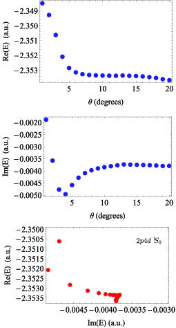
Figure 1: (Color online) Illustration of the CI+MBPT+CRM method for locating the $2p4d\,^{1}\!S_{0}$ resonance. The upper (central) panel shows dependence of the real (imaginary) part of the energy on the CRM rotation angle $\theta$. The bottom panel shows the corresponding trajectory in the complex plane. The kink in the trajectory marks the position of the resonance.

Our numerical results are compiled in Table 2. We tabulate energies, widths, and strengths of DR resonances falling within a 0.6 eV range above the $1s^{2}2s$ threshold. In this table, we also compare our values with the previous theoretical results of Ref. Mannervik et al. (1998). The energies are also compared with the NIST recommended values Ralchenko et al. (2008). We find that the overall agreement for energy positions is excellent and does not deviate by more than 2-3 meV. Detailed consideration reveals that the NIST recommended values for the position of the $2p4d\,^{3}\!P_{J}$ resonance differ both from our and Ref. Mannervik et al. (1998) predictions by as much as 13 meV. Even more strikingly, both our and Ref. Mannervik et al. (1998) predictions disagree with the NIST recommended value by a very large value of 147 meV for the position of the $2pd4\,^{1}\!F_{3}$ resonance.

Among 21 tabulated resonance positions, there is only one large disagreement between our work and theory of Ref. Mannervik et al. (1998): this happens for the $2p4d\,^{1}\!S_{0}$ resonance where the two calculations differ by 34 meV. Considering an excellent agreement for other 20 resonances between the two calculations, such a disagreement may indicate a typographical mistake in Ref. Mannervik et al. (1998). Ref. Mannervik et al. (1998) reports the following experimental positions of the resonances: 0.182 eV for $2p4d\,^{3}D$, 0.244 eV for the unresolved $2p4f\,^{1,3}\!F$, 0.438 eV for $2p4f\,^{3}\!D$, and 0.578 eV for $2p4d\,^{1}\!P$ with experimental uncertainty of 5 meV. All of these values are in agreement with our theoretical predictions.

A comparison of resulting autoionizing widths between our and Ref. Mannervik et al. (1998) calculations indicates a good agreement for broad resonances. The agreement for narrow ( width $<0.5$ meV) is less satisfying. Experimentally, the width of such resonances is determined by the experimental convolution function and no definitive conclusions can be drawn on the basis of theory-experiment comparison. Notice, that the $2p4d^{3}D$ and $2p4f^{1,3}F$ resonances were resolved in the experiment Mannervik et al. (1998). The calculated rate in Ref. Mannervik et al. (1998) was larger than the experimental one by 50%. It was not clear whether the source of the disagreement was theory or experiment. Perhaps, our disagreement for the width of narrow resonances with theory Mannervik et al. (1998) may indicate enhanced sensitivity to details of theoretical treatment. While there are discrepancies for the autoionizing widths of the narrow resonances, our CI+MBPT+CRM strengths of the resonances compare well with calculations of Ref. Mannervik et al. (1998) (see Table 2).

IV Conclusion

To summarize, we report developing a new method for computing properties of low-energy resonances in dielectronic recombination. A high-precision description of low-energy resonances is particularly challenging as it is sensitive to correlations. At the same time, uncertainties in the positions of the resonances drastically affect practically important recombination rates in low-temperature plasmas. Our theoretical approach is based on combining configuration-interaction method with many-body perturbation theory and complex rotation method (CI+MBPT+CRM). The method is ab initio relativistic. To gauge the accuracy of the developed CI+MBPT+CRM approach, we computed low-energy resonances in Be-like carbon. We find a good agreement with the earlier high-precision study by Mannervik et al. (1998). While here we studied a divalent ion, our developed methodology and computational toolbox is well suited for exploring resonances in systems with several valence electrons outside a closed-shell core.

Acknowledgements — We would like to thank D. Savin and E. Lindroth for discussions and Frank Greenhalgh for comments on the manuscript. This work was supported in part by the US NSF and by the US NASA under Grant/Cooperative Agreement No. NNX07AT65A issued by the Nevada NASA EPSCoR program.

Table 2: Ab initio values of energies (relative to the $1s^{2}2s\ ^{2}$S_1/2 threshold), the widths and strengths of resonances within 0.6 eV above the ionization limit of C III. The computed values are compared with theoretical results of Mannervik et al., (see Table I in Ref. Mannervik et al. (1998)) and NIST recommended energies Ralchenko et al. (2008).

			Energy (eV)			Width (meV)		Strength (10-20 eV cm2)
Term		$J$	Present	NISTRalchenko et al. (2008)	Ref.Mannervik et al. (1998)	Present	Ref.Mannervik et al. (1998)	Present	Ref.Mannervik et al. (1998)
$2p4d$	3Do	1	0.179	0.181	0.176	0.1	0.09	10.3	11.2
		2	0.183	0.181	0.177	0.005	0.18	17.2	18.5
		3	0.183	0.181	0.180	0.005	0.08	22.5	25.4
$2p4f$	1F	3	0.238		0.236	0.45	0.10	5.7	6.0
	3F	2	0.242	0.239	0.240	0.05	0.001	3.8	3.9
		3	0.243	0.241	0.242	0.6	0.25	5.3	5.5
		4	0.245	0.245	0.243	0.4	0.33	6.8	7.1
$2p4d$	3Po	0	0.291	0.279	0.292	50	52	1.1	1.3
		1	0.289	0.279	0.289	50	52	3.2	3.7
		2	0.284	0.279	0.285	50	52	4.7	5.8
$2p4f$	3G	3	0.353		0.351	117	115	3.1	3.3
		4	0.356		0.353	117	115	3.9	4.2
		5	0.365		0.360	117	115	4.7	5.1
	1G	4	0.379		0.375	118	115	3.1	3.2
	3D	1	0.435	0.433	0.433	1.1	1.01	1.2	1.2
		2	0.431	0.432	0.430	1.1	1.01	2.0	2.0
		3	0.427	0.425	0.426	1.2	1.01	2.8	2.8
	1D	2	0.451		0.452	0.6	0.22	1.8	1.8
$2p4d$	1Fo	3	0.461	0.314	0.460	232	236	7.4	8.5
$2p4p$	1S	0	0.451		0.485	202	221	0.2	0.2
$2p4d$	1Po	1	0.583		0.586	44	46	1.9	2.0

References

- Kallman and Palmeri (2007) T. R. Kallman and P. Palmeri, Rev. Mod. Phys. 79, 79 (2007), eprint arXiv:astro-ph/0610423.
- Pindzola et al. (2005) M. S. Pindzola, D. C. Griffin, and N. R. Badnell, in Springer Handbook of Atomic, Molecular, and Optical Physics, edited by G. W. F. Drake (Springer, New York, New York, 2005), pp. 829–834, 2nd ed.
- Parpia et al. (1996) F. A. Parpia, C. Froese Fischer, and I. P. Grant, Com. Phys. Comm. 94, 249 (1996).
- Hibbert (1975) A. Hibbert, Com. Phys. Comm. 9, 141 (1975).
- Fischer et al. (1997) C. F. Fischer, T. Brage, and P. Jonsson, Computational stomic structure - an MCHF approach, (Bristol: IOP) (1997).
- Badnell (1986) N. R. Badnell, J. Phys. B 19, 3827 (1986).
- Savin et al. (2003) D. Savin, S. Kahn, G. Gwinner, M. Grieser, R. Repnow, G. Saathoff, D. Schwalm, A. Wolf, A. Muller, S. Schippers, et al., Astrophys. J. Suppl. S. 147, 421 (2003).
- Schippers et al. (2004) S. Schippers, M. Schnell, C. Brandau, S. Kieslich, A. Muller, and A. Wolf, Astron. Astrophys. 421, 1185 (2004).
- Savin et al. (2006) D. W. Savin, G. Gwinner, M. Grieser, R. Repnow, M. Schnell, D. Schwalm, A. Wolf, S.-G. Zhou, S. Kieslich, A. Muller, et al., The Astrophysical Journal 642, 1275 (2006).
- Lindroth (1994) E. Lindroth, Phys. Rev. A 49, 4473 (1994).
- Mannervik et al. (1998) S. Mannervik, D. DeWitt, L. Engstrom, J. Lidgerg, E. Lindroth, R. Schuch, and W. Zong, Phys. Rev. Lett. 81, 313 (1998).
- Lindroth et al. (2001) E. Lindroth, H. Danared, P. Glans, Z. Pesic, M. Tokman, G. Vikor, and R. Schuch, Phys. Rev. Lett. 86, 5027 (2001).
- Tokman et al. (2002) M. Tokman, N. Eklow, P. Glans, E. Lindroth, R. Schuch, G. Gwinner, D. Schwalm, A. Wolf, A. Hoffknecht, A. Muller, et al., Phys. Rev. A 66, 012703/1 (2002).
- Lindgren and Morrison (1986) I. Lindgren and J. Morrison, Atomic Many–Body Theory (Springer–Verlag, Berlin, 1986), 2nd ed.
- Derevianko et al. (2008) A. Derevianko, S. G. Porsev, and K. Beloy, Phys. Rev. A 78, 010503(R) (2008).
- Dzuba (2008) V. A. Dzuba, Phys. Rev. A 78, 042502 (2008).
- Porsev et al. (2009) S. G. Porsev, K. Beloy, and A. Derevianko, Phys. Rev. Lett. 102, 181601 (2009).
- Dzuba et al. (1996) V. A. Dzuba, V. V. Flambaum, and M. G. Kozlov, Phys. Rev. A 54, 3948 (1996).
- Dzuba and Johnson (1998) V. A. Dzuba and W. R. Johnson, Phys. Rev. A 57, 2459 (1998).
- Kozlov et al. (2001) M. G. Kozlov, S. G. Porsev, and W. R. Johnson, Phys. Rev. A 64, 052107 (2001), eprint arXiv: physics/0105090.
- Dzuba (2005) V. A. Dzuba, Phys. Rev. A 71, 032512 (2005).
- Derevianko (2001) A. Derevianko, Phys. Rev. Lett. 87, 023002 (2001).
- Beloy and Derevianko (2008) K. Beloy and A. Derevianko, Comp. Phys. Comm. 179, 310 (2008).
- Reihardt (1982) W. P. Reihardt, Ann. Rev. Phys. Chem. 33, 223 (1982).
- Fokkema et al. (1996) D. R. Fokkema, G. L. G. Sleijpen, and H. A. van der Vorst (1996), preprint 941, Department of Mathematics, Utrecht University, URL http://www.math.ruu.nl/people/sleijpen/.
- Ralchenko et al. (2008) Y. Ralchenko, A. E. Kramida, J. Reader, and NIST ASD Team, NIST atomic spectra database (version 3.1.4) (2008), URL http://physics.nist.gov/asd3.