DESY 10-043 ISSN 0418-9833

March 2010

Diffractive Dijet Photoproduction
in $ep$ Collisions at HERA

H1 Collaboration

Measurements are presented of single and double-differential dijet cross sections in diffractive photoproduction based on a data sample with an integrated luminosity of $47\ {\rm pb^{-1}}$. The events are of the type $ep\rightarrow eXY$, where the hadronic system $X$ contains at least two jets and is separated by a large rapidity gap from the system $Y$, which consists of a leading proton or low-mass proton excitation. The dijet cross sections are compared with QCD calculations at next-to-leading order and with a Monte Carlo model based on leading order matrix elements with parton showers. The measured cross sections are smaller than those obtained from the next-to-leading order calculations by a factor of about $0.6$. This suppression factor has no significant dependence on the fraction $x_{\gamma}$ of the photon four-momentum entering the hard subprocess. Ratios of the diffractive to the inclusive dijet cross sections are measured for the first time and are compared with Monte Carlo models.

Submitted to Eur. Phys. J. C

F.D. Aaron^5,49, C. Alexa⁵, V. Andreev²⁵, S. Backovic³⁰, A. Baghdasaryan³⁸, E. Barrelet²⁹, W. Bartel¹¹, K. Begzsuren³⁵, A. Belousov²⁵, J.C. Bizot²⁷, V. Boudry²⁸, I. Bozovic-Jelisavcic², J. Bracinik³, G. Brandt¹¹, M. Brinkmann^12,51, V. Brisson²⁷, D. Bruncko¹⁶, A. Bunyatyan^13,38, G. Buschhorn^26,†, L. Bystritskaya²⁴, A.J. Campbell¹¹, K.B. Cantun Avila²², K. Cerny³², V. Cerny^16,47, V. Chekelian²⁶, A. Cholewa¹¹, J.G. Contreras²², J.A. Coughlan⁶, J. Cvach³¹, J.B. Dainton¹⁸, K. Daum^37,43, M. Deák¹¹, B. Delcourt²⁷, J. Delvax⁴, E.A. De Wolf⁴, C. Diaconu²¹, M. Dobre^12,51, V. Dodonov¹³, A. Dossanov²⁶, A. Dubak^30,46, G. Eckerlin¹¹, V. Efremenko²⁴, S. Egli³⁶, A. Eliseev²⁵, E. Elsen¹¹, A. Falkiewicz⁷, L. Favart⁴, A. Fedotov²⁴, R. Felst¹¹, J. Feltesse^10,48, J. Ferencei¹⁶, D.-J. Fischer¹¹, M. Fleischer¹¹, A. Fomenko²⁵, E. Gabathuler¹⁸, J. Gayler¹¹, S. Ghazaryan¹¹, A. Glazov¹¹, L. Goerlich⁷, N. Gogitidze²⁵, M. Gouzevitch¹¹, C. Grab⁴⁰, A. Grebenyuk¹¹, T. Greenshaw¹⁸, B.R. Grell¹¹, G. Grindhammer²⁶, S. Habib¹¹, D. Haidt¹¹, C. Helebrant¹¹, R.C.W. Henderson¹⁷, E. Hennekemper¹⁵, H. Henschel³⁹, M. Herbst¹⁵, G. Herrera²³, M. Hildebrandt³⁶, K.H. Hiller³⁹, D. Hoffmann²¹, R. Horisberger³⁶, T. Hreus^4,44, F. Huber¹⁴, M. Jacquet²⁷, X. Janssen⁴, L. Jönsson²⁰, A.W. Jung¹⁵, H. Jung^11,4, M. Kapichine⁹, J. Katzy¹¹, I.R. Kenyon³, C. Kiesling²⁶, M. Klein¹⁸, C. Kleinwort¹¹, T. Kluge¹⁸, A. Knutsson¹¹, R. Kogler²⁶, P. Kostka³⁹, M. Kraemer¹¹, J. Kretzschmar¹⁸, A. Kropivnitskaya²⁴, K. Krüger¹⁵, K. Kutak¹¹, M.P.J. Landon¹⁹, W. Lange³⁹, G. Laštovička-Medin³⁰, P. Laycock¹⁸, A. Lebedev²⁵, V. Lendermann¹⁵, S. Levonian¹¹, K. Lipka^11,51, B. List¹², J. List¹¹, N. Loktionova²⁵, R. Lopez-Fernandez²³, V. Lubimov²⁴, A. Makankine⁹, E. Malinovski²⁵, P. Marage⁴, Ll. Marti¹¹, H.-U. Martyn¹, S.J. Maxfield¹⁸, A. Mehta¹⁸, A.B. Meyer¹¹, H. Meyer³⁷, J. Meyer¹¹, S. Mikocki⁷, I. Milcewicz-Mika⁷, F. Moreau²⁸, A. Morozov⁹, J.V. Morris⁶, M.U. Mozer⁴, M. Mudrinic², K. Müller⁴¹, Th. Naumann³⁹, P.R. Newman³, C. Niebuhr¹¹, A. Nikiforov¹¹, D. Nikitin⁹, G. Nowak⁷, K. Nowak⁴¹, J.E. Olsson¹¹, S. Osman²⁰, D. Ozerov²⁴, P. Pahl¹¹, V. Palichik⁹, I. Panagoulias^l,11,42, M. Pandurovic², Th. Papadopoulou^l,11,42, C. Pascaud²⁷, G.D. Patel¹⁸, E. Perez^10,45, A. Petrukhin¹¹, I. Picuric³⁰, S. Piec¹¹, H. Pirumov¹⁴, D. Pitzl¹¹, R. Plačakytė¹¹, B. Pokorny³², R. Polifka³², B. Povh¹³, V. Radescu¹⁴, N. Raicevic³⁰, A. Raspiareza²⁶, T. Ravdandorj³⁵, P. Reimer³¹, E. Rizvi¹⁹, P. Robmann⁴¹, R. Roosen⁴, A. Rostovtsev²⁴, M. Rotaru⁵, J.E. Ruiz Tabasco²², S. Rusakov²⁵, D. Šálek³², D.P.C. Sankey⁶, M. Sauter¹⁴, E. Sauvan²¹, S. Schmitt¹¹, L. Schoeffel¹⁰, A. Schöning¹⁴, H.-C. Schultz-Coulon¹⁵, F. Sefkow¹¹, R.N. Shaw-West³, L.N. Shtarkov²⁵, S. Shushkevich²⁶, T. Sloan¹⁷, I. Smiljanic², Y. Soloviev²⁵, P. Sopicki⁷, D. South⁸, V. Spaskov⁹, A. Specka²⁸, Z. Staykova¹¹, M. Steder¹¹, B. Stella³³, G. Stoicea⁵, U. Straumann⁴¹, D. Sunar⁴, T. Sykora⁴, G. Thompson¹⁹, P.D. Thompson³, T. Toll¹¹, T.H. Tran²⁷, D. Traynor¹⁹, P. Truöl⁴¹, I. Tsakov³⁴, B. Tseepeldorj^35,50, J. Turnau⁷, K. Urban¹⁵, A. Valkárová³², C. Vallée²¹, P. Van Mechelen⁴, A. Vargas Trevino¹¹, Y. Vazdik²⁵, M. von den Driesch¹¹, D. Wegener⁸, E. Wünsch¹¹, J. Žáček³², J. Zálešák³¹, Z. Zhang²⁷, A. Zhokin²⁴, H. Zohrabyan³⁸, and F. Zomer²⁷

¹ I. Physikalisches Institut der RWTH, Aachen, Germany
² Vinca Institute of Nuclear Sciences, Belgrade, Serbia
³ School of Physics and Astronomy, University of Birmingham, Birmingham, UK^b
4 Inter-University Institute for High Energies ULB-VUB, Brussels and Universiteit Antwerpen, Antwerpen, Belgium^c
5 National Institute for Physics and Nuclear Engineering (NIPNE) , Bucharest, Romania^m
6 Rutherford Appleton Laboratory, Chilton, Didcot, UK^b
7 Institute for Nuclear Physics, Cracow, Poland^d
8 Institut für Physik, TU Dortmund, Dortmund, Germany^a
9 Joint Institute for Nuclear Research, Dubna, Russia
¹⁰ CEA, DSM/Irfu, CE-Saclay, Gif-sur-Yvette, France
¹¹ DESY, Hamburg, Germany
¹² Institut für Experimentalphysik, Universität Hamburg, Hamburg, Germany^a
13 Max-Planck-Institut für Kernphysik, Heidelberg, Germany
¹⁴ Physikalisches Institut, Universität Heidelberg, Heidelberg, Germany^a
15 Kirchhoff-Institut für Physik, Universität Heidelberg, Heidelberg, Germany^a
16 Institute of Experimental Physics, Slovak Academy of Sciences, Košice, Slovak Republic^f
17 Department of Physics, University of Lancaster, Lancaster, UK^b
18 Department of Physics, University of Liverpool, Liverpool, UK^b
19 Queen Mary and Westfield College, London, UK^b
20 Physics Department, University of Lund, Lund, Sweden^g
21 CPPM, Aix-Marseille Université, CNRS/IN2P3, Marseille, France
²² Departamento de Fisica Aplicada, CINVESTAV, Mérida, Yucatán, México^j
23 Departamento de Fisica, CINVESTAV IPN, México City, México^j
24 Institute for Theoretical and Experimental Physics, Moscow, Russia^k
25 Lebedev Physical Institute, Moscow, Russia^e
26 Max-Planck-Institut für Physik, München, Germany
²⁷ LAL, Université Paris-Sud, CNRS/IN2P3, Orsay, France
²⁸ LLR, Ecole Polytechnique, CNRS/IN2P3, Palaiseau, France
²⁹ LPNHE, Université Pierre et Marie Curie Paris 6, Université Denis Diderot Paris 7, CNRS/IN2P3, Paris, France
³⁰ Faculty of Science, University of Montenegro, Podgorica, Montenegro^e
31 Institute of Physics, Academy of Sciences of the Czech Republic, Praha, Czech Republic^h
32 Faculty of Mathematics and Physics, Charles University, Praha, Czech Republic^h
33 Dipartimento di Fisica Università di Roma Tre and INFN Roma 3, Roma, Italy
³⁴ Institute for Nuclear Research and Nuclear Energy, Sofia, Bulgaria^e
35 Institute of Physics and Technology of the Mongolian Academy of Sciences, Ulaanbaatar, Mongolia
³⁶ Paul Scherrer Institut, Villigen, Switzerland
³⁷ Fachbereich C, Universität Wuppertal, Wuppertal, Germany
³⁸ Yerevan Physics Institute, Yerevan, Armenia
³⁹ DESY, Zeuthen, Germany
⁴⁰ Institut für Teilchenphysik, ETH, Zürich, Switzerland^i
41 Physik-Institut der Universität Zürich, Zürich, Switzerlandⁱ

⁴² Also at Physics Department, National Technical University, Zografou Campus, GR-15773 Athens, Greece
⁴³ Also at Rechenzentrum, Universität Wuppertal, Wuppertal, Germany
⁴⁴ Also at University of P.J. Šafárik, Košice, Slovak Republic
⁴⁵ Also at CERN, Geneva, Switzerland
⁴⁶ Also at Max-Planck-Institut für Physik, München, Germany
⁴⁷ Also at Comenius University, Bratislava, Slovak Republic
⁴⁸ Also at DESY and University Hamburg, Helmholtz Humboldt Research Award
⁴⁹ Also at Faculty of Physics, University of Bucharest, Bucharest, Romania
⁵⁰ Also at Ulaanbaatar University, Ulaanbaatar, Mongolia
⁵¹ Supported by the Initiative and Networking Fund of the Helmholtz Association (HGF) under the contract VH-NG-401.

^† Deceased

^a Supported by the Bundesministerium für Bildung und Forschung, FRG, under contract numbers 05H09GUF, 05H09VHC, 05H09VHF, 05H16PEA
^b Supported by the UK Science and Technology Facilities Council, and formerly by the UK Particle Physics and Astronomy Research Council
^c Supported by FNRS-FWO-Vlaanderen, IISN-IIKW and IWT and by Interuniversity Attraction Poles Programme, Belgian Science Policy
^d Partially Supported by Polish Ministry of Science and Higher Education, grant DPN/N168/DESY/2009
^e Supported by the Deutsche Forschungsgemeinschaft
^f Supported by VEGA SR grant no. 2/7062/ 27
^g Supported by the Swedish Natural Science Research Council
^h Supported by the Ministry of Education of the Czech Republic under the projects LC527, INGO-1P05LA259 and MSM0021620859
ⁱ Supported by the Swiss National Science Foundation
^j Supported by CONACYT, México, grant 48778-F
^k Russian Foundation for Basic Research (RFBR), grant no 1329.2008.2
^l This project is co-funded by the European Social Fund (75%) and National Resources (25%) - (EPEAEK II) - PYTHAGORAS II
^m Supported by the Romanian National Authority for Scientific Research under the contract PN 09370101

1 Introduction

Quantum Chromodynamics (QCD), as the gauge field theory of the strong interaction, reliably predicts scattering cross sections involving short distance partonic interactions. However, the vast majority of hadron-hadron scatterings take place through long-distance strong interactions, where no hard scales are present and perturbative QCD calculations are not possible. Prominent among these soft interactions are diffractive processes, in which the interacting hadrons remain intact or dissociate into low mass hadronic systems via an exchange which has vacuum quantum numbers, often referred to as a ‘pomeron’ [1]. Following the observation of diffractive $p\bar{p}$ collisions in which a hard scale is provided by high transverse momentum jets [2], it has become possible to describe some classes of diffractive processes in terms of partonic interactions [3]. More recently, diffractive deep-inelastic scattering (DDIS) processes at HERA [4], of the type $ep\rightarrow eXp$, have been studied in detail and have led to a new level of understanding of the properties and structure of the diffractive exchange. Developing this microscopic description of diffraction in terms of QCD and parton dynamics is a step towards a more complete understanding of the strong interaction.

In the framework of a collinear factorisation theorem [5] for hard scattering in semi-inclusive processes such as DDIS, diffractive parton distribution functions (DPDFs) may be defined. The DPDFs have similar properties to the standard parton distribution functions (PDFs) of the proton, but with the constraint that there be a leading proton present in the final state. This condition may be satisfied equivalently by the experimental signatures of either a leading proton [6, 7] or the presence of a large gap in the rapidity distribution of final state hadrons, separating an unobserved outgoing proton from the remainder of the hadronic final state [8, 7]. In various extractions using recent DDIS data [8, 9, 10, 11], the DPDFs have been found to be dominated by gluons. To good approximation they exhibit a ‘proton vertex factorisation’ property, whereby they vary only in normalisation with the four-momentum of the final state proton, the normalisation being well modelled using Regge phenomenology [12].

Given a knowledge of the DPDFs, perturbative QCD calculations are applicable to other DDIS observables. Such calculations have been successful in the prediction of jet [13, 14, 9] and heavy quark [15] production in DDIS at HERA. In both cases, next-to-leading order (NLO) QCD predictions using the DPDFs from [8] describe the measured cross sections well. However, as has long been anticipated [16, 5], DPDF-based predictions for hard diffractive processes such as dijet production in $p\bar{p}$ scattering fail by around an order of magnitude to describe the data [17, 18]. This factorisation breaking is generally attributed to absorptive corrections, corresponding to the destruction of the rapidity gap due to multiple interactions within a single event. Such effects are possible in $p\bar{p}$ scattering, where a beam remnant is present, in contrast to the electron scattering case in DDIS at HERA. A diversity of models of the absorptive corrections has developed [19, 20], several of which reproduce the approximate $10\%$ ‘rapidity gap survival probability’ observed in single diffractive $p\bar{p}$ scattering.

The issues of DPDF applicability and rapidity gap survival can be studied in $ep$ collisions at HERA in hard diffractive ‘photoproduction’, where the virtuality $Q^{2}$ of the exchange photon is close to zero. Under these circumstances, the photon can develop an effective partonic structure via $\gamma\rightarrow q\bar{q}$ fluctuations and further subsequent splittings [21]. In a leading order picture, there are thus two classes of hard photoproduction: ‘direct’ interactions, where the photon enters the hard scatter as a structureless object and ‘resolved’ interactions, where the photon interacts via its partonic structure and only a fraction $x_{\gamma}$ of its four-momentum participates in the hard subprocess. Resolved photoproduction interactions can be further divided into a ‘hadron-like’ contribution and an ‘anomalous’ or ‘point-like’ contribution, the latter arising from the inhomogeneous term in the DGLAP equation for the photon [22]. Interactions involving the hadron-like component resemble hadron-hadron scattering to a large extent and are therefore widely expected to exhibit gap destruction effects. The rapidity gap survival probability for these hadron-like processes has been estimated in a phenomenological model to be $0.34$ [23, 24]. The point-like contribution to photon structure is expected to be subject to smaller absorptive corrections than the hadron-like part [25]. In a recent model [24] a survival probability of around $0.7-0.8$ was obtained for diffractive dijet photoproduction, depending slightly on the jet transverse energies ($E_{T}^{\rm jet}$).

Previous H1 measurements of diffractive dijet photoproduction [13, 26] have found cross sections to be smaller than NLO theoretical predictions, suggesting rapidity gap survival probabilities of around $0.5$ with little dependence on $x_{\gamma}$. A recent ZEUS measurement at somewhat larger $E_{T}^{\rm jet}$ [27] yielded a larger survival probability, compatible with unity. It has been proposed that this apparent discrepancy may be resolved if the rapidity gap survival probability depends on the scale of the hard interaction, an idea which is supported to some extent by data [26, 27, 28]. Neither H1 nor ZEUS data provide any evidence for the expected $x_{\gamma}$ dependence of the rapidity gap survival probability.

A measurement of the ratio of the diffractive to the inclusive dijet photoproduction cross sections was proposed in [23, 25, 29] as a means of evaluating the gap survival probability. This ratio is expected to be relatively insensitive to the model of the photon parton densities and also offers cancellations of experimental systematics and higher order QCD corrections. A similar ratio was measured by the CDF collaboration [17] as a means of extracting effective $p\bar{p}$ DPDFs for comparison with HERA predictions and assessment of gap survival probabilities.

This paper reports diffractive dijet photoproduction cross section measurements based on a positron-proton scattering data sample with luminosity about a factor three larger than that previously published by H1 [26]. The larger sample makes double-differential measurements possible, giving greater detail on the dynamics of gap survival and allowing studies of the correlations between the kinematic variables. The hypothesis of an $E_{T}^{\rm jet}$ dependent rapidity gap survival probability is tested. The ratio of the diffractive to the inclusive dijet photoproduction cross sections is also extracted for the first time.

2 Kinematic Variables

Figures 1 (a) and (b) show leading order examples of direct and resolved diffractive dijet production. Denoting the four-vectors of the incoming positron, the incoming proton and the exchanged photon as $k$, $P$ and $q$, respectively, the standard DIS kinematics can be described in terms of the invariants

$$s\equiv(k+P)^{2}\hskip 36.98866ptQ^{2}\equiv-q^{2}\hskip 36.98866pty\equiv{{q\cdot P}\over{k\cdot P}}\hskip 36.98866ptx\equiv{{Q^{2}}\over{2\,q\cdot P}}\ .$$ (1)

Here, $s$ is the square of the total centre of mass energy of the collision, $Q^{2}$ is the photon virtuality, $y$ is the scattered positron inelasticity and $x$ is the fraction of the proton four-momentum carried by the quark coupling to the photon. These variables are related through $Q^{2}=s\,x\,y$ and to the invariant mass $W$ of the photon-proton system by

$$W\equiv\sqrt{(q+P)^{2}}\approx\sqrt{ys-Q^{2}}\ .$$ (2)

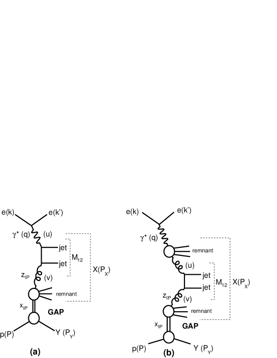
Figure 1: Leading order diagrams for diffractive dijet photoproduction at HERA. Diagrams (a) and (b) are examples of direct and resolved photon interactions, respectively.

Defining $P_{X}$ and $P_{Y}$ to be the four-vectors of the two distinct final state systems, where $Y$ may be either a proton or a low mass proton excitation, the diffractive kinematics are described by the variables

$$M_{X}^{2}\equiv P_{X}^{2}\hskip 36.98866ptM_{Y}^{2}\equiv P_{Y}^{2}\hskip 36.98866ptt\equiv(P-P_{Y})^{2}\hskip 36.98866ptx_{{I\!\!P}}\equiv{{q\cdot(P-P_{Y})}\over{q\cdot P}}\ .$$ (3)

Here, $M_{X}$ and $M_{Y}$ are the invariant masses of the systems $X$ and $Y$, $t$ is the squared four-momentum transfer at the proton vertex and $x_{{I\!\!P}}$ is the fraction of the longitudinal momentum of the proton transferred to the system $X$.

With $u$ and $v$ being the four-momenta of the particles entering the hard scatter from the photon and proton, respectively ($u=q$ in the direct photon case), the invariant mass $M_{12}$ of the dijet system and the fractional photon ($x_{\gamma}$) and pomeron ($z_{{I\!\!P}}$) longitudinal momenta entering the hard subprocess can be expressed as

$$M_{12}\equiv\sqrt{(u+v)^{2}}\hskip 36.98866ptx_{\gamma}\equiv{{P\cdot u}\over{P\cdot q}}\hskip 36.98866ptz_{{I\!\!P}}\equiv{{q\cdot v}\over{q\cdot(P-P_{Y})}}\ .$$ (4)

3 Theory and Models

3.1 Diffractive Dijet Photoproduction in the Factorisation Approach

Dijet electroproduction cross sections for $Q^{2}\rightarrow 0$ can be calculated in a fixed order QCD approach, assuming QCD collinear factorisation and neglecting any rapidity gap destruction effects, as a convolution of partonic cross sections, photon PDFs and DPDFs, according to

$$d\sigma(ep\rightarrow e+2\,{\rm jets}+X^{\prime}+Y)=\sum_{i,j}\int dy\,\,f_{\gamma/e}(y)\int dx_{\gamma}f_{j/\gamma}(x_{\gamma},\mu_{F}^{2})\ \otimes$$

$$\int dt\int dx_{{I\!\!P}}\int dz_{{I\!\!P}}\ d\hat{\sigma}(ij\rightarrow 2\,{\rm jets})\ f_{i/p}^{D}(z_{{I\!\!P}},\mu_{F}^{2},x_{{I\!\!P}},t)\ .$$ (5)

Here, the hadronic system $X^{\prime}$ corresponds to the remainder of the system $X$ after removing the two jets. The sum runs over all partons $i$ and $j$ that contribute, $f_{\gamma/e}$ is the equivalent flux of photons that emerge from the incoming lepton [30] and $f_{j/\gamma}$ are the photon PDFs ($f_{j/\gamma}=\delta(1-x_{\gamma})$ in the direct photon case). The hard partonic cross sections are denoted $\hat{\sigma}$, $f_{i/p}^{D}$ are the DPDFs of the proton and $\mu_{F}$ is the factorisation scale.

In this analysis, the GRV HO [31] parton densities are used to describe the structure of the resolved photon. The H1 2006 Fit B set is used for the DPDFs, obtained by the H1 collaboration in fits to inclusive DDIS data [8]. In the poorly constrained large $z_{{I\!\!P}}$ region, previous DDIS final state data [9, 26, 15] have shown a clear preference for these DPDFs over the Fit A set from [8]. Further DPDF sets from H1 (H1 2007 Fit Jets) [9] and ZEUS (ZEUS DPDF SJ) [7, 10] in which dijet data from DDIS are used to improve the sensitivity to the large $z_{{I\!\!P}}$ region, are also considered. All of these DPDF sets assume proton vertex factorisation, such that

$$f_{i/p}^{D}(z_{{I\!\!P}},\mu_{F}^{2},x_{{I\!\!P}},t)=f_{{I\!\!P}/p}(x_{{I\!\!P}},\,t)f_{i/{I\!\!P}}(z_{{I\!\!P}},\,\mu_{F}^{2})\ .$$ (6)

In the interpretation illustrated in figure 1, $f_{{I\!\!P}/p}(x_{{I\!\!P}},t)$ may be considered as a pomeron flux, parameterised using Regge phenomenology in the DPDF sets used here. The $f_{i/{I\!\!P}}$ factor then represents the parton densities of the pomeron. At relatively large values of $x_{{I\!\!P}}\,\raisebox{-3.01385pt}{$\stackrel{{\scriptstyle\textstyle>}}{{\sim}}$}\,0.01$ a small contribution from a sub-leading meson exchange is required in the DPDF fits. This is taken into account by adding a second term of the same form as equation 6, but with different parton densities and a flux factor which is suppressed as $x_{{I\!\!P}}\rightarrow 0$.

3.2 Next-to-leading Order Parton Level QCD Calculations

The dijet electroproduction cross sections (equation 3.1) are calculated at NLO of QCD using the program of Frixione et al. (FR) [32] adapted for diffractive applications as described in [33, 26]. In the FR program, the renormalisation and factorisation scales are set to be equal and both are taken here from the leading jet transverse energy, i.e $\mu_{R}=\mu_{F}=E_{T}^{\rm jet1}$. The NLO calculations are performed with the number of flavours fixed to 5 and the QCD scale parameter set to $\Lambda_{5}=0.228\ {\rm GeV}$, corresponding to a 2-loop $\alpha_{s}(M_{Z})=0.118$. The sensitivity of the calculated cross sections to the chosen $\mu_{R}$ and $\mu_{F}$ values is studied by varying both scales simultaneously by factors of $0.5$ and $2$. The NLO calculations were cross-checked with the program written by Klasen and Kramer [25], which yields consistent results [28, 34].

3.3 Monte Carlo Simulations

3.3.1 Corrections to the Data

A Monte Carlo (MC) simulation is used to correct the data for detector effects in obtaining cross sections at the level of stable hadrons. All MC samples are passed through a detailed simulation of the H1 detector response based on the GEANT program [35] and are subjected to the same reconstruction and analysis algorithms as are used for the data.

Diffractive dijet photoproduction events are generated using the RAPGAP MC generator [36] in the range $Q^{2}<0.01$ GeV² with the minimum transverse momentum of the partons entering the hard subprocess set to $\hat{p}_{T}^{min}=2~{}\mbox{GeV}$. RAPGAP is based on leading order QCD matrix elements with DGLAP parton showers. The H1 2006 fit B DPDFs and the GRV-G LO photon parton densities [31] are used at a factorisation scale given by $E_{T}^{\rm jet1}$. A sub-leading meson exchange is included in the DPDF simulation, though its contribution is smaller than $5\%$ in the kinematic range covered here.

The selection of diffractive events using the rapidity gap method (section 4.2) yields a sample which is dominated by elastically scattered protons, but which also contains an admixture of events in which the proton dissociates to low $M_{Y}$ states. The measurement is corrected to the region $M_{Y}<1.6\ {\rm GeV}$ and $|t|<1\ {\rm GeV^{2}}$ (section 4.3), using MC samples generated using the DIFFVM [37] program, with and without proton dissociation, following the method described in [8].

In order to estimate the small ($\sim 2\%$) contribution to the data sample from non-diffractive events which pass the diffractive selection, the PYTHIA MC generator [38] is used in photoproduction mode ($Q^{2}<0.01~{}\mbox{GeV}^{2}$). The PYTHIA model is also used to correct the inclusive photoproduction dijet measurement for detector effects when extracting the ratio of diffractive to inclusive cross sections. To estimate the model uncertainties on the corrections to the inclusive dijet cross section, a further MC sample is obtained using the HERWIG generator [39]. Multiple interaction models are included in both PYTHIA and HERWIG as described in section 3.3.2. With these settings, PYTHIA provides a good description of the shapes of the uncorrected inclusive dijet distributions, with a normalisation slightly larger than that of the data. The HERWIG MC underestimates the normalisation of the cross section by about a factor of two, but gives an acceptable description of the shapes of the measured distributions.

3.3.2 Corrections to Theoretical Models

For comparison with the diffractive measurements, it is necessary to convert the calculated NLO parton-level cross sections to the level of stable hadrons by evaluating effects due to initial and final state parton showering, fragmentation, hadronisation and the influence of beam remnants. The RAPGAP MC is used to compute the required ‘hadronisation correction’ factors to the diffractive dijet calculations. These factors are defined for each measured data point by

$$1+\delta_{hadr.}={{\sigma_{\rm dijet}^{\rm hadron}}\over{\sigma_{\rm dijet}^{\rm parton}}}\ .$$ (7)

They reduce the predicted cross sections by typically $15\%$ and are given for each data point in tables 2 and 4. The shape of the $x_{\gamma}$ distribution is most strongly affected by the hadronisation corrections, the main effect being the migration of some direct photon interactions, for which the cross section is large, to lower $x_{\gamma}$ values, substantially increasing the prediction in the interval $0.6<x_{\gamma}<0.8$.

Resolved photon interactions in inclusive dijet production [40] are poorly described by NLO calculations unless a model of multiple interactions (MI) within a single event is included in addition to the low transverse momentum beam remnant, QCD radiation and hadronisation contributions which are simulated in standard MC models. The PYTHIA MC generator is used to investigate the influence of MIs on inclusive dijet cross sections and hence on the diffractive-to-inclusive ratios. Several tunes of the PYTHIA model for multiple hard parton-parton scatterings are available. In the version used here (tune A in [38]), both the proton and the resolved photon have double-Gaussian matter distributions. The minimum transverse momentum down to which secondary partonic scatterings are calculated depends on the impact parameter of the collision and is governed by a regularisation scale $p_{\perp 0}=1.2\ {\rm GeV}$ [38].

Multiple hard partonic interactions are not simulated in the HERWIG MC. Instead, an empirically motivated soft multiple interaction model [39] is used. The probability of such activity in a given event is set to $0.25$.

4 Experimental Procedure

4.1 The H1 Detector

A detailed description of the H1 detector can be found elsewhere [41]. Here, a brief account is given of the detector components most relevant to the present analysis. The H1 coordinate system is defined such that the origin is at the nominal $ep$ interaction point and the polar angle $\theta=0^{\circ}$ and the positive $z$ axis correspond to the direction of the outgoing proton beam. The region $\theta<90^{\circ}$, which has positive pseudorapidity $\eta=-\ln\tan\theta/2$, is referred to as the ‘forward’ hemisphere.

The ep interaction point in H1 is surrounded by a central tracking region, which includes silicon strip detectors as well as two large concentric drift chambers. These chambers cover a pseudorapidity region of $-1.5<\eta<1.5$ and have a transverse momentum resolution of $\sigma(P_{T})/P_{T}=0.006P_{T}/{\rm GeV}\oplus 0.02$. They also provide triggering information. The central tracking detectors are surrounded by a finely segmented liquid argon (LAr) sampling calorimeter covering $-1.5<\eta<3.4$. Its resolution is $\sigma/E=0.11/\sqrt{E/{\rm GeV}}\oplus 0.01$ for electrons and photons and $\sigma/E=0.50/\sqrt{E/{\rm GeV}}\oplus 0.02$ for hadrons, as measured in test beams [42]. The central tracker and LAr calorimeter are placed inside a large superconducting solenoid, which produces a uniform magnetic field of $1.16$ T. The backward region $-4<\eta<-1.4$ is covered by a lead-scintillating fibre calorimeter (SpaCal) with electromagnetic and hadronic sections.

Information from the central tracker and the LAr and SpaCal calorimeters is combined using an energy flow algorithm to obtain the hadronic final state (HFS) [43]. The hadronic energy scale is known to $3\%$ for this analysis [34].

Photoproduction events are selected by tagging positrons scattered through very small angles, corresponding to quasi-real photon emission, using a crystal Čerenkov calorimeter at $z=-33~{}\mbox{m}$ (electron tagger). The luminosity is measured via the Bethe-Heitler bremsstrahlung process $ep\rightarrow ep\gamma$, the final state photon being detected in another crystal calorimeter at $z=-103~{}\mbox{m}$.

A set of drift chambers around $z=6.5~{}\mbox{m}$ comprise the forward muon detector (FMD). The proton remnant tagger (PRT) is a set of scintillators surrounding the beam pipe at $z=26~{}\mbox{m}$. These detectors, used together with the most forward part of the LAr, are efficient in the identification of very forward energy flow and are used to select events with large rapidity gaps near to the outgoing proton direction.

4.2 Event Selection, Kinematic and Jet Reconstruction

The analysis is based on a sample of integrated luminosity $47\ {\rm pb^{-1}}$, collected by H1 in 1999 and 2000 with proton and positron beam energies of $920\ {\rm GeV}$ and $27.5\ {\rm GeV}$, respectively. The events are triggered on the basis of a scattered positron signal in the electron tagger and at least three high transverse momentum tracks in the drift chambers of the central tracker.

The event inelasticity $y$ and hence the invariant mass $W$ of the photon-proton system are reconstructed using the scattered positron energy $E_{e^{\prime}}$ measured in the electron tagger according to

$$y=1-{{E_{e^{\prime}}}\over{E_{e}^{beam}}}\hskip 36.98866ptW=\sqrt{s\,y}\ ,$$ (8)

where $E_{e}^{beam}$ is the positron beam energy. The geometric acceptance of the electron tagger limits the measurement to $Q^{2}<0.01~{}\mbox{GeV}^{2}$ and intermediate values of $y$.

The reconstructed hadronic final state objects (section 4.1) are subjected to the $k_{T}$ longitudinally invariant jet algorithm [44], applied in the laboratory frame with parameters $R=1$ and $E_{T}^{\rm jet,min}=2.5\,\,\mbox{GeV}$. To facilitate comparisons with the NLO calculations, different cuts are placed on the transverse energies $E_{T}^{\rm jet1}$ and $E_{T}^{\rm jet2}$ of the leading and next-to-leading jets, respectively. As well as these variables, the jet properties are studied in terms of the variables

$${\left|\Delta\eta^{\rm jets}\right|}={\left|\eta^{\rm jet1}-\eta^{\rm jet2}\right|}\hskip 36.98866pt\left<\eta^{\rm jets}\right>={{1}\over{2}}\left(\eta^{\rm jet1}+\eta^{\rm jet2}\right)\ ,$$ (9)

obtained from the laboratory frame pseudorapidities of the jet axes. With $J^{(1)}$ and $J^{(2)}$ denoting the four-momenta of the two jets, hadron level estimators of the dijet invariant mass and of $x_{\gamma}$ are obtained from

$$M_{12} = \sqrt{2\,J^{(1)}\cdot J^{(2)}}\hskip 36.98866ptx_{\gamma}^{\rm jets}={{\Sigma_{jets}(E_{i}-P_{z,i})}\over{\Sigma_{HFS}(E_{i}-P_{z,i})}}\ ,$$ (10)

where the sums labelled ‘HFS’ and ‘jets’ run over all hadronic final state objects and those included in the jets, respectively.

The diffractive event selection is based on the presence of a large forward rapidity gap. The pseudorapidity of the most forward cluster in the LAr calorimeter with energy above $400$ MeV is required to satisfy $\eta^{max}<3.2$. The activity in the PRT and the FMD is required not to exceed that typical of noise levels as obtained from randomly triggered events. These requirements ensure that the analysed sample is dominated by elastically scattered protons at small $|t|$, with a small admixture of events with leading neutrons and low $M_{Y}$ baryon excitations, collectively referred to here as ‘proton dissociation’ contributions.

The diffractive kinematics are reconstructed using

$$x_{{I\!\!P}}={{\Sigma_{HFS}(E_{i}+P_{z,i})}\over{2E_{p}^{beam}}}\hskip 36.98866ptM_{X}=\sqrt{s\,y\,x_{{I\!\!P}}}\ ,$$ (11)

where $E_{p}^{beam}$ is the proton beam energy. A cut on $x_{{I\!\!P}}$ is applied to ensure good containment of the system $X$ and to suppress sub-leading exchange contributions. A hadron level estimator for the momentum fraction $z_{{I\!\!P}}$ is obtained using

$$z_{{I\!\!P}}^{\rm jets} = {{\Sigma_{jets}(E_{i}+P_{z,i})}\over{\Sigma_{HFS}(E_{i}+P_{z,i})}}\ .$$ (12)

The kinematic range in which the diffractive dijet measurement is performed is specified in table 1. The inclusive measurement phase space is defined by these conditions, with the requirements relaxed on the diffractive variables $x_{{I\!\!P}}$, $z^{\rm jets}_{{I\!\!P}}$, $M_{Y}$ and $t$. Except where measurements are made explicitly as a function of $z_{{I\!\!P}}^{\rm jets}$, the $z_{{I\!\!P}}^{\rm jets}>0.8$ region is excluded from the diffractive analysis. This improves the reliability of the comparison between data and theoretical predictions, since the DPDF sets used are not valid at the largest $z_{{I\!\!P}}$ values. After applying all selection criteria, about $3600$ out of roughly $200000$ inclusive dijet photoproduction events are used in the diffractive analysis. A more detailed description of the analysis can be found in [34].

Diffractive and Inclusive Measurements
$Q^{2}<0.01\ {\rm GeV^{2}}$		$0.3\ <y<\ 0.65$
$E_{T}^{\rm jet1}>5\ {\rm GeV}$		$E_{T}^{\rm jet2}>4\ {\rm GeV}$
$-1<\eta^{\rm jet1}<2$		$-1<\eta^{\rm jet2}<2$
Diffractive Measurement
$x_{{I\!\!P}}<0.03$		$z^{\rm jets}_{{I\!\!P}}<0.8$
$M_{Y}<1.6\ {\rm GeV}$		$\left|t\right|<1\ {\rm GeV^{2}}$

Table 1: Kinematic ranges of the diffractive and inclusive measurements.

4.3 Cross Section Measurement

The diffractive differential cross section is measured in each bin $i$ of a variable $x$ using the formula

$$\left({{{\rm d}\sigma}\over{{\rm d}x}}\right)_{i} = {{N^{data}_{i}/\varepsilon^{trig}_{i}-N^{MC,bgd}_{i}}\over{A_{i}~{}\Delta^{x}_{i}}~{}{\cal L}}\cdot~{}\frac{1}{C^{pdiss}}\ .$$ (13)

Here, $N^{data}_{i}$ is the raw number of reconstructed events passing the selection criteria listed in section 4.2 and $\varepsilon^{trig}_{i}$ is the trigger efficiency, obtained by reference to an independently triggered sample and parameterised as a function of the multiplicity of charged particle tracks. The trigger efficiency averaged over the full measurement range is $0.86$. The non-diffractive background contribution obtained from the PYTHIA MC simulation is denoted $N^{MC,bgd}_{i}$ and does not extend beyond the few percent level for any of the measured data points. The factor $A_{i}$ corrects the measurement for detector effects, including migrations between bins, to the level of stable hadrons. It is calculated from the RAPGAP MC and has an average value of $0.31$ for the diffractive analysis, most of the losses being due to the limited electron tagger acceptance of $0.40$ integrated over the measured $y$ range. The bin width is denoted $\Delta^{x}_{i}$, ${\cal L}$ is the luminosity of the data sample and $C^{pdiss}=0.94\pm 0.07$, evaluated using the DIFFVM MC, corrects the measurement to the chosen range of $M_{Y}$ and $t$ (table 1). In the inclusive analysis the cross section is obtained analogously to equation 13 except for the $N^{MC,bgd}$ and $C^{pdiss}$ terms, which are not relevant.

4.4 Systematic Uncertainties

Uncertainties are evaluated for all significant sources of possible systematic bias. These sources are summarised for the diffractive analysis below, together with their corresponding influences on the total diffractive cross section.

Energy Scale:

The energy scale of the HFS measurement is tested using the momentum balance constraint between the precisely reconstructed positron and the HFS in neutral current DIS events. Dedicated data and MC samples are analysed and found to agree to better than $3\%$. The effect of a relative $3\%$ change in the energy of the HFS between the data and the MC is a $9.6\%$ shift to the total diffractive dijet cross section. This arises mainly from changes in the migration corrections across the minimum $E_{T}^{\rm jet}$ values and the maximum $x_{{I\!\!P}}$ value of the measurement. The energy scale uncertainties are thus highly correlated between the bins of the differential cross section measurements.

Large Rapidity Gap Selection:

A fraction of the events in the kinematic range of the analysis (table 1) give rise to hadronic activity in the forward detectors or at pseudorapidities beyond those allowed by the $\eta^{max}$ cut in the LAr calorimeter. Corrections for this inefficiency of the large rapidity gap selection are made using the RAPGAP MC simulation. The uncertainties in the correction factors are assessed through a study of forward energy flow in a sample of dijet photoproduction events with leading protons tagged in the H1 Forward Proton Spectrometer [6]. RAPGAP is found to describe these migrations to within 10% [45, 26], which translates into a $2.9\%$ uncertainty on the measured total cross section and uncertainties which are correlated between bins of the differential distributions.

Proton Dissociation:

The model dependence uncertainty on the proton dissociation correction factor ($C^{pdiss}$ in equation 13) is obtained by varying the elastic and proton dissociation cross sections and the proton dissociation $M_{Y}$ and $t$ dependences in the DIFFVM MC samples, following [8]. The largest effect arises from varying the ratio of the proton-elastic to the proton-dissociative cross sections between $0.5$ and $2$. The resulting uncertainty on the measured cross section is $7\%$.

Model Dependence:

The influence of the model assumptions on the acceptance and bin migration corrections ($A_{i}$ in equation 13), is determined in the diffractive analysis by varying the kinematic distributions in the RAPGAP simulation within the limits allowed by maintaining an acceptable description of the uncorrected data. The following variations are implemented by reweighting each MC event according to the value of generator level kinematic variables, leading to the quoted systematic uncertainties on the total cross section.

• The $x_{{I\!\!P}}$ distribution is reweighted by $x_{{I\!\!P}}^{\pm 0.2}$, leading to a $6.0\%$ uncertainty.

• The $z_{{I\!\!P}}^{\rm jets}$ distribution is reweighted by $z_{{I\!\!P}}^{{\rm jets}\ \pm 0.3}$, leading to a $4.8\%$ uncertainty.

• The $x_{\gamma}^{\rm jets}$ distribution is reweighted by $x_{\gamma}^{{\rm jets}\ \pm 0.3}$, leading to a $0.6\%$ uncertainty.

• The $E_{T}^{\rm jet1}$ distribution is reweighted by $E_{T}^{\rm jet1\ \pm 0.4}$, leading to a $0.8\%$ uncertainty.

• The $t$ distribution is reweighted by $e^{\pm 2t}$, leading to a $4.4\%$ uncertainty.

• The $y$ distribution is reweighted by $y^{\pm 0.3}$, leading to a $0.2\%$ uncertainty.

Electron Tagger Acceptance:

A dedicated procedure external to this analysis is used to obtain the electron tagger acceptance [46]. The integrated acceptance over the full $y$ range is known to $5\%$, which affects the cross section normalisation.

Trigger Efficiency:

The procedure for parameterising the trigger efficiency ($\varepsilon^{trig}_{i}$ in equation 13) leads to a $5\%$ uncertainty. This covers the observed deviations of the parameterisation from the measured efficiencies as a function of all variables relevant to the analysis. This uncertainty is treated as being uncorrelated between data points.

Luminosity:

The measurement of the integrated luminosity has an uncertainty of $1.5\%$. This translates directly into a $1.5\%$ normalisation uncertainty on the measured cross sections.

Non-diffractive background:

A $50\%$ normalisation variation is applied to the non-diffractive background contribution given by the PYTHIA MC model ($N^{MC,bgd}$ in equation 13). The effect of this change is correlated between the data points and leads to a $1\%$ uncertainty on the total cross section.

Forward Detector Noise:

Fluctuations in the FMD noise, leading to losses in the large rapidity gap event selection, are evaluated for each run using randomly triggered events. The standard deviation in the run-by-run distribution of the correction factors is used to derive a $0.5\%$ normalisation uncertainty on the measured cross sections. Noise in the PRT detector is negligible.

A similar procedure is followed to evaluate the systematic uncertainties in the inclusive dijet analysis. The uncertainties associated with the large rapidity gap selection and the model dependence are no longer relevant. Instead, comparisons between the PYTHIA and HERWIG MCs are used determine a $2\%$ model dependence uncertainty on the acceptance correction when integrated over the full phase space studied. The inclusive cross section systematics are dominated by a contribution at the $10\%$ level from the HFS energy scale uncertainty. However, when forming the ratio of diffractive to inclusive cross sections, this error source cancels to good approximation, the residual uncertainty being less than $1\%$. The largest remaining contribution to the systematic uncertainty on the cross section ratio arises from the model dependence.

The total systematic uncertainty on each data point is formed by adding the individual contributions in quadrature. In the figures and tables that follow, the systematic uncertainties are separated into two categories: those which are uncorrelated between data points (the model dependence and trigger efficiency) and those which lead to correlations between data points (all other sources).

5 Results

5.1 Diffractive Dijet Cross Sections

Cross sections are measured integrated over the full kinematic range specified in table 1 and also single- and double-differentially as a function of a variety of variables which are sensitive to the overall event structure, the hard subprocess and the presence of remnants of the virtual photon and the diffractive exchange. The measured differential cross sections, which correspond to averages over the specified measurement intervals, are given numerically in tables 2 and 4, where the experimental uncertainties and hadronisation corrections applied to the NLO calculations are also listed. Tables 3 and 5 contain the ratios of the measurements to the NLO calculations, obtained using the FR framework (section 3.2) and the H1 2006 Fit B DPDFs (referred to in the following as FR Fit B).

5.1.1 Integrated Cross Section

The total diffractive dijet positron-proton cross section integrated over the full measured kinematic range is

$$\sigma^{tot}_{data}=295\pm 6~{}(\mbox{stat.})\pm 58~{}(\mbox{syst.})~{}~{}\mbox{pb}\ .$$ (14)

The ratio of this result to the corresponding FR Fit B NLO prediction is

$$\sigma^{tot}_{data}/\sigma^{tot}_{NLO}=0.58\pm 0.01~{}(\mbox{stat.})\pm 0.12~{}(\mbox{syst.})\pm 0.14~{}(\mbox{scale})\pm 0.09~{}(\mbox{DPDF})\ ,$$ (15)

where the statistical and systematic uncertainties originate from the measurement. The scale uncertainty corresponds to the effect of simultaneously varying the renormalisation and factorisation scales from their central values, $\mu_{R}=\mu_{F}=E_{T}^{\rm jet1}$, by a factor of two in either direction. This large ($25\%$) scale uncertainty arises due to the relatively low $E_{T}^{\rm jet1}$ range of this analysis, and is the limiting factor in the comparison between data and theory. The DPDF uncertainty is obtained using the method of [47], by propagating the eigenvector decomposition of the fit uncertainties. If the H1 2006 Fit B DPDFs are replaced by the H1 2007 Fit Jets DPDFs, the result is $\sigma^{tot}_{data}/\sigma^{tot}_{NLO}=0.64$, which is inside the quoted DPDF uncertainty. Using ZEUS DPDF SJ, a compatible result of $\sigma^{tot}_{data}/\sigma^{tot}_{NLO}=0.70$ is obtained.

Adding all uncertainties in quadrature, the ratio result in equation 15 implies at the $2\sigma$ level that the NLO QCD calculation, neglecting any gap destruction effects, yields a larger diffractive dijet photoproduction cross section than that measured. It confirms the result of a previous H1 analysis in a very similar kinematic range [26] and is broadly as expected from theoretical calculations of rapidity gap survival probabilities [23, 29].

5.1.2 Single-Differential Cross Sections

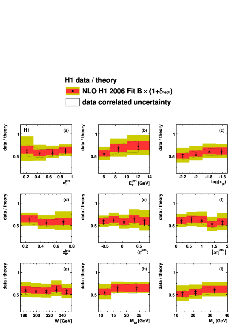
Figure 3: Ratios of the single-differential cross sections to the corresponding NLO QCD predictions based on the FR framework and the H1 2006 Fit B DPDF set, corrected for hadronisation effects. See the caption of figure 2 for further details.

Figure 2 shows the diffractive dijet cross section measured single-differentially in $x_{\gamma}^{\rm jets}$, $E_{T}^{\rm jet1}$, $\log x_{{I\!\!P}}$, $z_{{I\!\!P}}^{\rm jets}$, $\left<\eta^{\rm jets}\right>$, $\left|\Delta\eta^{\rm jets}\right|$, $W$, $M_{12}$ and $M_{X}$, in the phase space defined in table 1. In figure 2(d), the $z_{{I\!\!P}}^{\rm jets}<0.8$ requirement is relaxed and the cross section measured for the region $z_{{I\!\!P}}^{\rm jets}>0.8$ is shown without theoretical comparisons, since the DPDFs are not defined (see section 4.2). To allow a more detailed shape comparison between the data and the predictions, ratios of the measured differential cross sections to the FR Fit B calculations are plotted in figure 3. These ratios may be taken as measurements of the dependence of the rapidity gap survival probability on the kinematic variables.

Figures 2 and 3 show that the suppression by around a factor of $0.6$ of the data with respect to the FR Fit B NLO calculations has at most a weak dependence on the kinematic variables. Notably, within the uncertainties there is no dependence on $x_{\gamma}^{\rm jets}$ (figure 3(a)), in contrast to theoretical predictions for the rapidity gap survival probability [23, 29]. The largest dependence of the central values of the measured ratios on any of the variables appears in the cross section differential in $E_{T}^{\rm jet1}$ (figure 3(b)). Although not well established by the current data, this dependence is compatible with previous data [26, 27, 28]. The $E_{T}^{\rm jet1}$ dependence is investigated further in section 5.1.3.

The measured cross sections in figure 2 are also compared with a prediction obtained using the RAPGAP MC generator (section 3.3.1), which does not contain any model of rapidity gap destruction. The shapes of the measured cross sections are well described and the normalisation is only slightly lower than that of the data. However the scale uncertainty in this model is rather large and the same model undershoots diffractive dijet measurements in DIS [26, 9], where factorisation is expected to hold.

In [27], the ZEUS collaboration presented an analysis of diffractive dijet photoproduction data with $E_{T}^{\rm jet1}>7.5\ {\rm GeV}$, which is most readily compared with the second and third $E_{T}^{\rm jet1}$ intervals in figures 2(b) and 3(b). However, even for $E_{T}^{\rm jet1}>7.5\ {\rm GeV}$, a direct comparison between H1 and ZEUS data is not possible, since the ZEUS analysis covers a wider $y$ range and cuts on the second jet at an $E_{T}^{\rm jet2}$ value of $6.5\ {\rm GeV}$, larger than the value used here. An indirect comparison can be made on the basis of ratios of the data to NLO theoretical calculations using the H1 Fit B DPDFs. ZEUS obtains a result of around $0.9$ for this ratio, which is compatible with the result for $E_{T}^{\rm jet1}>7.5\ {\rm GeV}$ obtained here, within the large combined uncertainties.

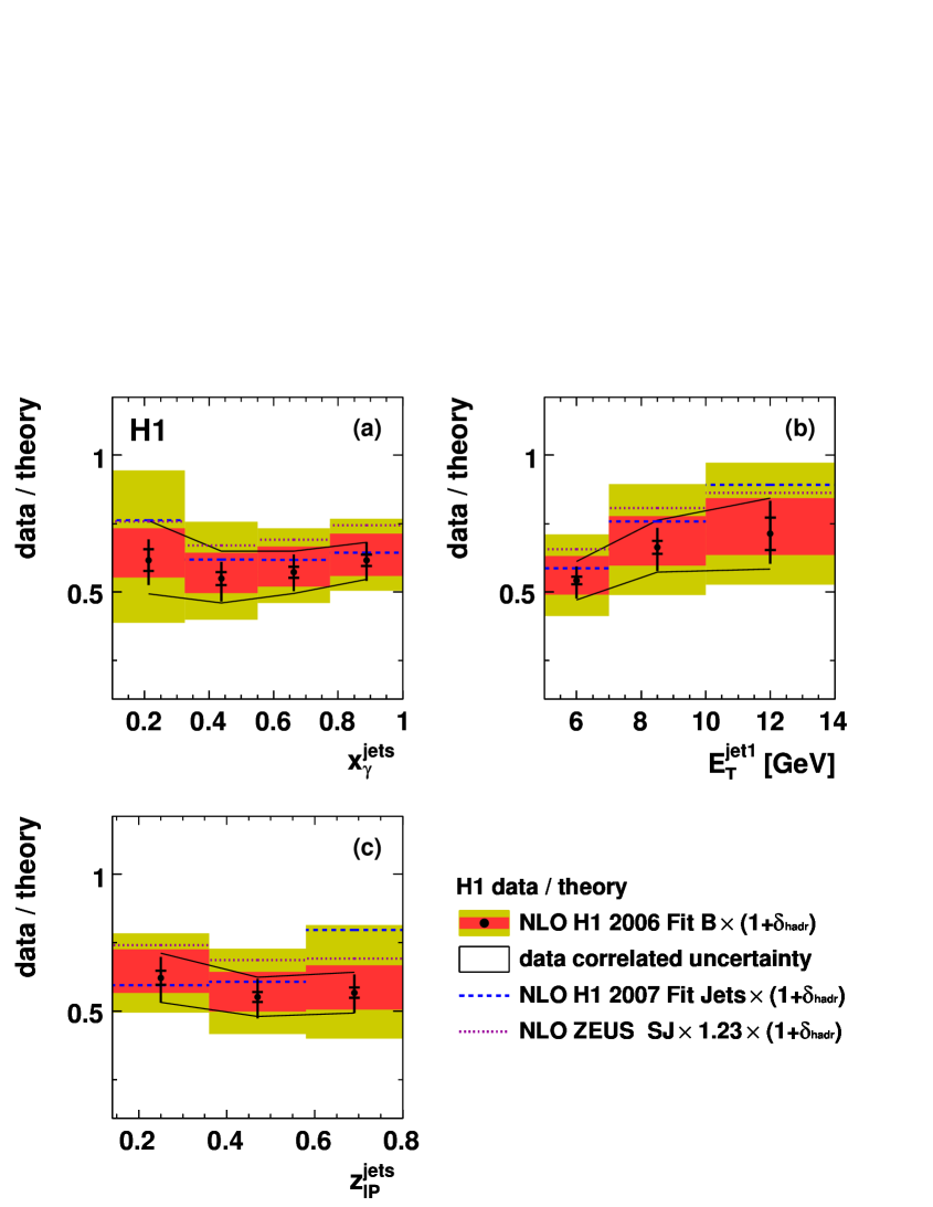
Figure 4: Ratios of the single-differential cross sections to the corresponding NLO QCD predictions based on the FR framework, corrected for hadronisation effects, for a subset of variables. Results obtained with H1 2006 Fit B set of diffractive parton densities are compared with those from H1 2007 DPDF Fit Jets and from the ZEUS DPDF SJ fit. The latter is scaled by a factor of $1.23$ [6] to convert its coverage from elastic protons only ($Y=p$) to $M_{Y}<1.6\ {\rm GeV}$. See the caption of figure 2 for further details.

As discussed in detail in [8, 9], the error bands on the DPDFs extracted from inclusive diffraction alone do not include uncertainties due to parton parameterisation choices and thus do not reflect the full uncertainties, particularly in the large $z_{{I\!\!P}}^{\rm jets}$ region. To give a complementary indication of the possible range of variation, comparisons between the ratios obtained with the H1 2006 Fit B DPDFs, the H1 2007 Fit Jets DPDFs and ZEUS DPDF SJ fit are shown for a subset of variables ($x_{\gamma}^{\rm jets}$, $E_{T}^{\rm jet1}$ and $z_{{I\!\!P}}^{\rm jets}$) in figure 4. The ZEUS DPDFs lead to ratios which are uniformly $10-15\%$ larger than those obtained with H1 2006 Fit B, with no strong dependence on any of the kinematic variables. The deviation of the H1 2007 Fit Jets result from the H1 2006 Fit B result extends beyond the DPDF error band for $z_{{I\!\!P}}^{\rm jets}>0.6$, which is correlated with a somewhat stronger dependence of the ratio of data to theory on $E_{T}^{\rm jet1}$ and a slightly different shape at low $x_{\gamma}^{\rm jets}$.

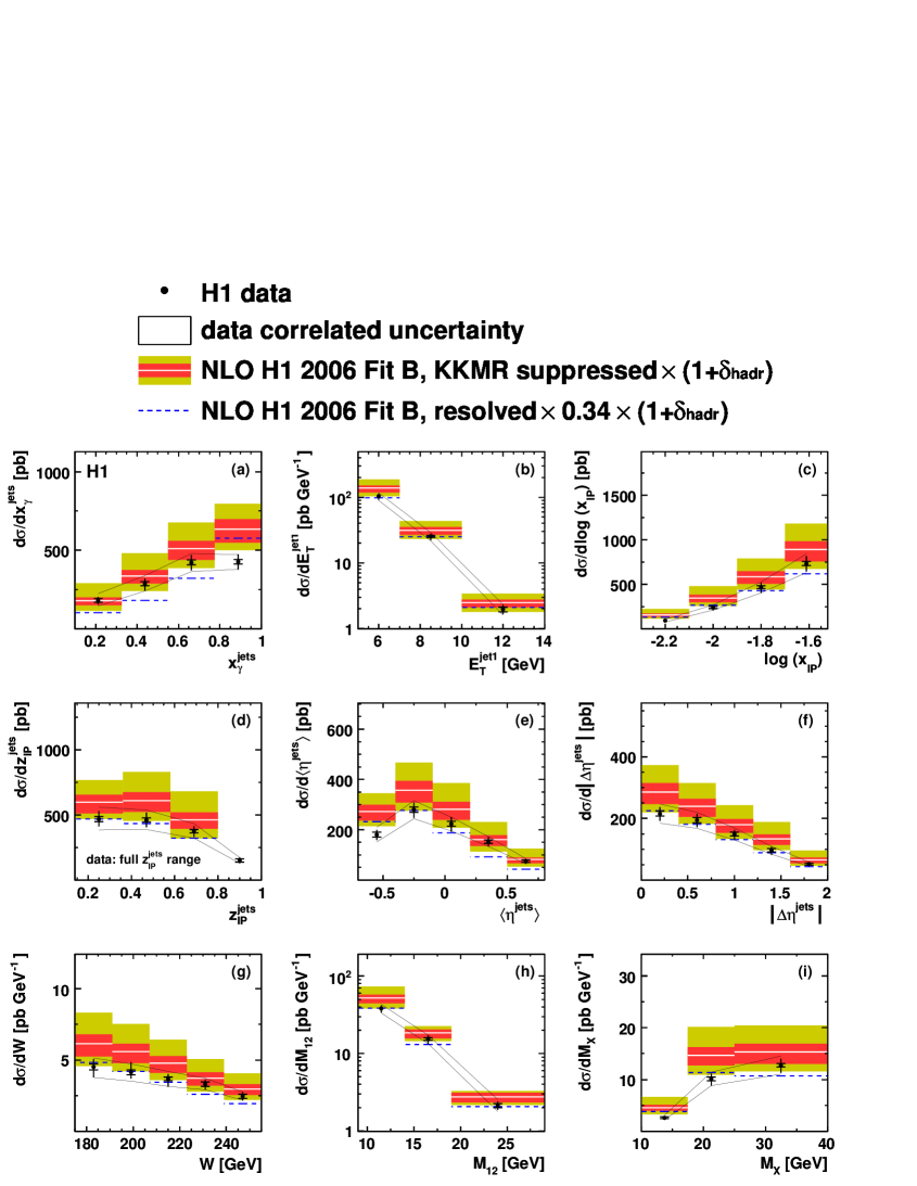
Figure 5: Single-differential diffractive dijet photoproduction cross sections as in figure 2. The FR theoretical prediction for resolved photons is modified by applying the scale factors from the KKMR model for point-like interactions (‘KKMR suppressed’) [24] or for hadron-like interactions (‘resolved $\times 0.34$’) [23]. The direct photon contribution is left unchanged in both cases. See the caption of figure 2 for further details.

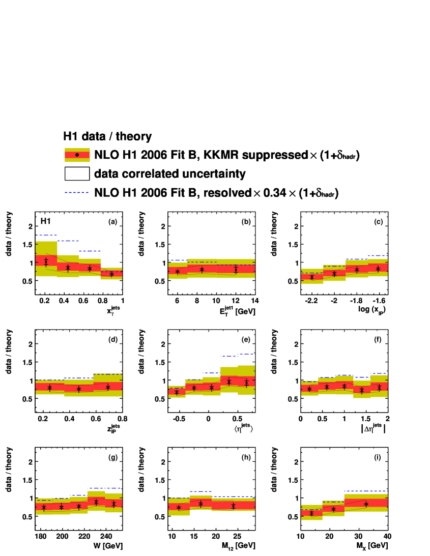
Figure 6: Ratios of the single-differential cross sections to the corresponding NLO QCD predictions based on the FR framework and the H1 2006 Fit B DPDF set, corrected for hadronisation effects. The FR theoretical prediction for resolved photons is modified by applying the scale factors from the KKMR model for point-like interactions (‘KKMR suppressed’) [24] or for hadron-like interactions (‘resolved $\times 0.34$’) [23]. The direct photon contribution is left unchanged in both cases. See the caption of figure 2 for further details.

According to the RAPGAP model, approximately half of the cross section in the kinematic range studied arises from each of the direct and resolved photon-induced contributions. The decomposition of photoproduction processes into direct and resolved interactions is not uniquely defined beyond LO. When modelling rapidity gap survival probabilities in the following, the resolved photon contribution is defined to correspond exactly to that which is calculated using the photon structure function. Following the calculation using an absorptive model of a gap survival probability of $0.34$ for the hadron-like component of resolved photoproduction [23], previous H1 data [26] were compared in [25] with predictions in which the full resolved photon contribution was suppressed by this factor, the direct photon contribution being left unsuppressed. In a later analysis [29], this procedure was extended to NLO. The conclusions of these previous studies are confirmed in figures 5 and 6 through a similar comparison of the current data with NLO calculations in which the resolved photon contribution is globally suppressed by a factor of 0.34. The overall normalisation of this calculation is in good agreement with the data. However, the shapes of some of the differential distributions are not well reproduced. In particular, there is a variation by more than a factor of two in the ratio of data to theory as a function of $x_{\gamma}^{\rm jets}$ (figure 6a).

The distinction between point-like and hadron-like resolved photon interactions recently developed in [24] leads to a significantly weaker predicted suppression in the kinematic range of the current analysis. The data are compared with this refined ‘KKMR’ model under the approximation of completely neglecting hadron-like resolved photon contributions, which, according to the authors, become dominant only for $x_{\gamma}^{\rm jets}<0.1$ [50], beyond the range of the current analysis. The rapidity gap survival probabilities obtained in [24] for point-like photon interactions using the GRV HO photon PDFs are applied to all resolved photon interactions. Interactions involving quarks and gluons from the photon are thus suppressed by factors of $0.71$ and $0.53$, respectively. The quark-initiated contribution is dominant throughout the measured range, such that the rapidity gap survival probability in the model is approximately $0.7$ for resolved photon interactions and $1$ for direct photon interactions.

Figure 5 shows the comparison between the measured single differential cross sections and the NLO QCD predictions, with the resolved photon contribution scaled according to the KKMR model. The corresponding ratios of data to theoretical predictions are shown in figure 6. The overall normalisation of the KKMR-based calculation is larger than that of the data, but is compatible within the large uncertainties. Many of the distributions studied are well described in shape ($E_{T}^{\rm jet1}$, $z_{{I\!\!P}}^{\rm jets}$, $\left|\Delta\eta^{\rm jets}\right|$, $W$ and $M_{12}$). The data thus agree with the prediction [29] that the $E_{T}^{\rm jet1}$ dependence of the data/theory ratio flattens if the resolved photon contribution alone is suppressed. However, there remains a variation in the ratio of data to the KKMR model with $x_{\gamma}^{\rm jets}$ and to a lesser extent with $\left<\eta^{\rm jets}\right>$, $x_{{I\!\!P}}$ and $M_{X}$. A comparison of figures 3 and 6 shows that the shapes of the differential cross sections are generally better described with a global suppression factor than with a survival probability applied to resolved photon interactions only.

5.1.3 Double-Differential Cross Sections

To study further the dynamics of rapidity gap suppression and their dependence on the nature of the photon interaction, cross sections are measured double differentially in two regions of $x_{\gamma}^{\rm jets}$, which are enriched with either resolved ($x_{\gamma}^{\rm jets}<0.75$) or direct ($x_{\gamma}^{\rm jets}>0.75$) photon processes. Using the RAPGAP MC model with the GRV-G LO photon PDFs, the $x_{\gamma}^{\rm jets}<0.75$ region is estimated to contain $77\%$ resolved photon interactions integrated over the measurement region (table 1), with a $75\%$ direct photon contribution for $x_{\gamma}^{\rm jets}>0.75$.

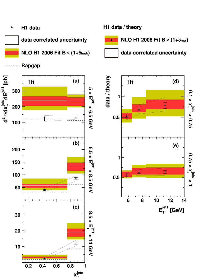
Figure 7: (a)-(c) Double-differential cross section ${\rm d}^{2}\sigma/{\rm d}E_{T}^{\rm jet1}{\rm d}x_{\gamma}^{\rm jets}$ as a function of $x_{\gamma}^{\rm jets}$, compared with NLO QCD and RAPGAP predictions. (d)-(e) Ratio of the double-differential cross section to the NLO prediction as a function of $E_{T}^{\rm jet1}$. See the caption of figure 2 for further details.

In figures 7(a)-(c), measurements are presented of the double-differential dijet cross section ${\rm d}^{2}\sigma/{\rm d}E_{T}^{\rm jet1}{\rm d}x_{\gamma}^{\rm jets}$ for three $E_{T}^{\rm jet1}$ ranges in the resolved and direct photon-enriched $x_{\gamma}^{\rm jets}$ intervals. The data are compared with the FR Fit B calculations and with the RAPGAP MC predictions. Due to kinematic constraints, the resolved-enriched cross section at low $x_{\gamma}^{\rm jets}$ falls most rapidly as $E_{T}^{\rm jet1}$ increases. There is a suggestion that this $E_{T}^{\rm jet1}$ dependence in the resolved-enriched region is stronger for the NLO QCD theory than for the data. In the direct-enriched high $x_{\gamma}^{\rm jets}$ region, the cross section falls more slowly with $E_{T}^{\rm jet1}$ and the dependence in the data is similar to that predicted by the NLO calculation. These features are illustrated further in figures 7 (d)-(e), where the ratios of the data to the NLO theory from figures 7 (a)-(c) are presented as a function of $E_{T}^{\rm jet1}$ in the resolved and direct photon-enriched $x_{\gamma}^{\rm jets}$ regions, respectively.

The significance of the $E_{T}^{\rm jet1}$ dependence in the resolved-enriched region (figure 7 (d)) is evaluated through a $\chi^{2}$ test. All uncertainties are taken into account in this procedure, though the main contribution comes from the statistical and uncorrelated systematic uncertainties on the data, the remaining uncertainties changing only the normalisation of the ratio to first approximation. A test of the hypothesis that there is no $E_{T}^{\rm jet1}$ dependence yields a $\chi^{2}$ value of 1.36, with two degrees of freedom, corresponding to an $E_{T}^{\rm jet1}$ variation at the 73% confidence level. The suppression of the data relative to the NLO prediction in the direct-enriched large $x_{\gamma}^{\rm jets}$ region is, within errors, independent of $E_{T}^{\rm jet1}$ (figure 7 (e)). Figures 7 (d)-(e) thus indicate that any $E_{T}^{\rm jet1}$ dependence of the data-to-theory ratio in figure 3(b) is driven primarily by resolved photon interactions. An $E_{T}^{\rm jet1}$ dependence of the gap survival probability is predicted in the KKMR model, due to variations in the size of the $q\bar{q}$ dipole produced by the point-like photon splitting, and hence in the absorptive correction. However the predicted effect is small ($4\%$ as $E_{T}^{\rm jet1}$ changes from $5\ {\rm GeV}$ to $7.5\ {\rm GeV}$). Figures 3(d)-(e) also indicate that when $E_{T}^{\rm jet1}$ becomes large, the suppression in the direct region may be stronger than that in the resolved region, which is not expected in any model. The large uncertainties permit statistical fluctuations in the data or small inadequacies in the theory as possible explanations.

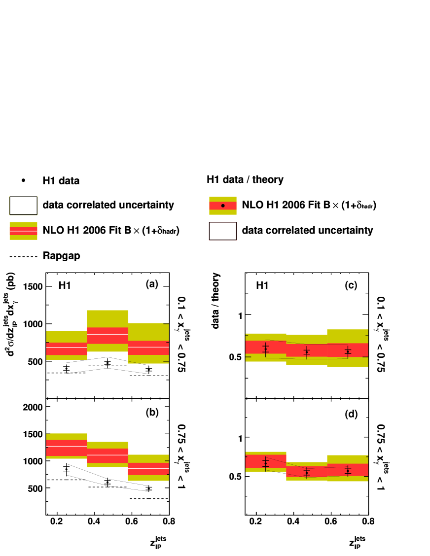
Figure 8: (a)-(b) Double-differential cross section ${\rm d}^{2}\sigma/{\rm d}z_{{I\!\!P}}^{\rm jets}{\rm d}x_{\gamma}^{\rm jets}$. (c)-(d) Ratio of the measured double-differential cross section to the NLO prediction using the H1 2006 Fit B and H1 2007 Fit Jets DPDFs. See the caption of figure 2 for further details.

In figure 8, the cross section is shown double differentially in $z_{{I\!\!P}}^{\rm jets}$ and $x_{\gamma}^{\rm jets}$. The measured cross section is compared with the NLO theory as a function of $z_{{I\!\!P}}^{\rm jets}$ in two bins of $x_{\gamma}^{\rm jets}$ in figures 8 (a)-(b) and the ratios of data to theoretical predictions are shown in figures 8 (c)-(d). The NLO calculations describe the measured shapes rather well, with no evidence for any variation of the suppression factor between any of the measurement ranges. The gap survival probability in a region where there are small or no remnants of either the photon or the diffractive exchange (highest $z_{{I\!\!P}}^{\rm jets}$ bin in figure 8d) is thus similar to that where both remnants are significant (lowest $z_{{I\!\!P}}^{\rm jets}$ bin in figure 8c). This remains the case when the H1 2007 Fit Jets DPDFs are used in place of H1 2006 Fit B. In both figures 7 and 8, the RAPGAP MC prediction gives a satisfactory description of the shapes of the double differential cross sections, the normalisation being slightly lower than that of the data.

5.2 Ratios of Diffractive to Inclusive Cross Sections

Measurements of ratios of diffractive to inclusive dijet photoproduction cross sections have been proposed [23, 25, 29] as a further test of gap survival issues. Their potential advantages over straight-forward diffractive measurements lie in the partial cancellations of some experimental systematics and of theoretical uncertainties due to the photon structure and factorisation and renormalisation scale choices. The sensitivity to absorptive effects of diffractive-to-inclusive ratios is thus potentially superior to that of pure diffractive cross sections. For the ratio extraction presented here, inclusive dijet cross sections are measured using data collected in the same period as the diffractive sample. The experimental method and systematic error treatment for the inclusive case is described in section 4. It is identical to the diffractive measurement method, with the exception of the large rapidity gap requirements.

At the relatively low transverse energies studied in the present analysis, underlying event effects have a large influence on jet cross sections in inclusive photoproduction [40]. Here, the PYTHIA and HERWIG MC models are used to correct the inclusive data for detector effects, with MI included as described in section 3.3.2. The two models agree rather well on the corrections to be applied to the data. The average of the results with the two models is therefore used to calculate the corrections and the uncertainty. The latter is taken from the difference between the results with the two models and is relatively small ($2\%$ when integrated over the full measured range).

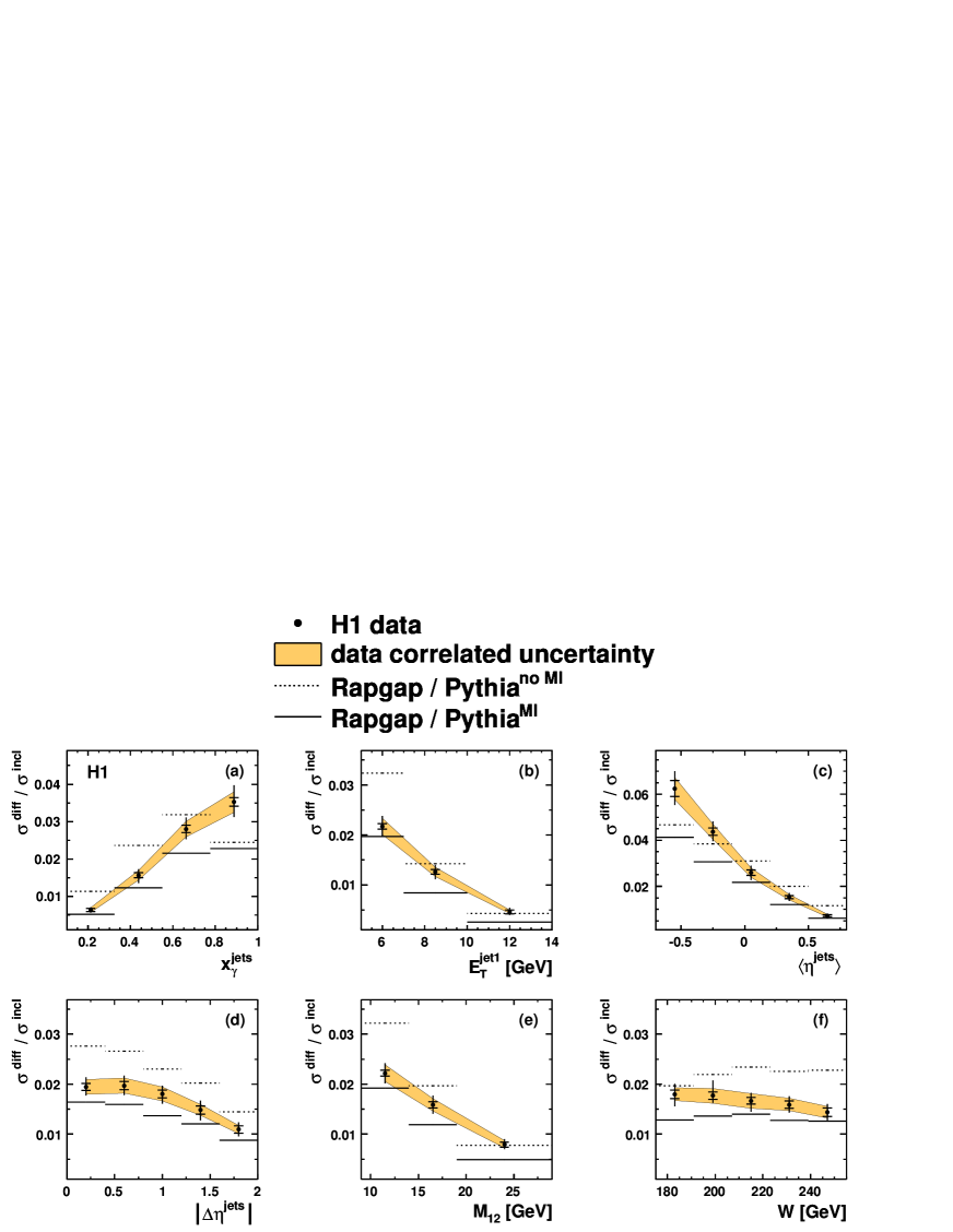
Figure 9: Ratios of diffractive to inclusive single-differential cross sections as a function of (a) $x_{\gamma}^{\rm jets}$, (b) $E_{T}^{\rm jet1}$, (c) $\left<\eta^{\rm jets}\right>$, (d) $\left|\Delta\eta^{\rm jets}\right|$, (e) $M_{12}$ and (f) $W$. The data points are shown with inner error bars corresponding to statistical uncertainties and outer error bars representing statistical and uncorrelated uncertainties added in quadrature. The correlated systematic errors are indicated by the hatched bands. The dashed lines represent the predictions from the ratio of the RAPGAP diffractive to the PYTHIA inclusive MC models without a multiple parton interaction model included in PYTHIA. The solid lines correspond to the same ratio of MC models with the inclusion of multiple parton interactions in PYTHIA.

The ratios of diffractive to inclusive single-differential dijet cross sections are given numerically in table 6 and are shown in figure 9 as a function of $x_{\gamma}^{\rm jets}$, $E_{T}^{\rm jet1}$, $\left<\eta^{\rm jets}\right>$, $\left|\Delta\eta^{\rm jets}\right|$, $M_{12}$ and $W$. Due to the partial or complete cancellations of some error sources when forming the ratio, the correlated uncertainties are reduced compared with those for the diffractive distributions.

Since they give adequate descriptions of the diffractive and inclusive data, respectively, the RAPGAP and PYTHIA MC models are used to assess the relative sensitivity of the diffractive-to-inclusive ratio to the gap survival and MI effects. With no MI effects included in the PYTHIA model, the description of the inclusive data is poor and the ratio of RAPGAP to PYTHIA exceeds the data by a factor of around 1.5. As expected, this factor becomes smaller as $E_{T}^{\rm jet1}$ increases. However, the shape of the prediction also differs from that of the ratio data for most of the other variables studied, in particular $x_{\gamma}^{\rm jets}$.

The inclusion of the PYTHIA MI model changes the predicted inclusive cross sections, and hence the ratios, substantially. The ratio of RAPGAP to PYTHIA then gives an improved description of the shapes of the distributions. The MI effects alter the predicted ratio by a factor of 0.5 at low $x_{\gamma}^{\rm jets}$, where the resolved photon remnant is most important. As expected, there is little effect in the direct photon-dominated large $x_{\gamma}^{\rm jets}$ region. The normalisation of the ratio of the models when MI are included is smaller than that of the data. This partially reflects the RAPGAP description of the diffractive data (figure 2) and is partially due to an overshoot in the PYTHIA description of the inclusive data.

The fractional reduction in the predicted inclusive cross section when MI are introduced in the PYTHIA model is comparable to the magnitude of the gap survival suppression factor in the diffractive data (section 5.1). The uncertainties in modelling the MI are large and difficult to quantify. The precision with which gap survival issues can be unfolded from MI complications in the ratio of diffractive to inclusive data is correspondingly poor. Therefore no strong conclusions can be drawn with our current understanding of MI, despite the relatively good precision of the data.

6 Summary

Single and double-differential cross sections are measured for diffractive dijet photoproduction and are compared with predictions based on NLO QCD calculations using different sets of DPDFs. Ratios of the measured to the predicted differential cross sections are also studied.

The total diffractive dijet cross section is overestimated by the NLO QCD theory by about a factor of two, which is consistent with previous H1 measurements [26]. The shapes of the single-differential cross sections are well described when the H1 2006 DPDF Fit B partons are used. A good overall description of the differential cross sections is obtained by applying a global suppression factor of $0.58\pm 0.21$ to the NLO calculations. As in similar previous analyses [26, 27, 28], there is a suggestion of a dependence of the rapidity gap survival probability on $E_{T}^{\rm jet1}$, though the significance of this effect is not large.

If only the resolved photon contribution in the calculation is suppressed by a factor of $0.34$, as predicted for hadron-like resolved photon interactions [23], the overall normalisation of the NLO QCD prediction agrees well with the data. However, the description of the $x_{\gamma}^{\rm jets}$ distribution, which best distinguishes direct from resolved photon interactions, becomes poor. If rapidity gap survival probabilities expected for point-like resolved photons are applied instead [24], the overall normalisation is acceptable and the $E_{T}^{\rm jet1}$ dependence of the data is better described. However, the description of the $x_{\gamma}^{\rm jets}$ dependence remains problematic.

The analysis of the double-differential cross section ${\rm d}^{2}\sigma/{\rm d}E_{T}^{\rm jet1}{\rm d}x_{\gamma}^{\rm jets}$ indicates that the $E_{T}^{\rm jet1}$ dependence of the data/theory ratio originates from the resolved photon-enriched region of $x_{\gamma}^{\rm jets}$. However, the data are also consistent with no dependence on $E_{T}^{\rm jet1}$ for either of the $x_{\gamma}^{\rm jets}$ regions studied. The ratio of the data to the NLO theory for the double-differential cross section ${\rm d}^{2}\sigma/{\rm d}z_{{I\!\!P}}^{\rm jets}{\rm d}x_{\gamma}^{\rm jets}$ is constant within errors throughout the region studied, indicating that the gap survival probability is insensitive to the presence or nature of remnants of either the photon or the diffractive exchange.

Measurements of the ratio of diffractive to inclusive single-differential cross sections are presented as a function of several variables. The influence of multiple interaction effects in the inclusive data is large in the kinematic range studied here. The large uncertainties in modelling these multiple interactions preclude strong conclusions about rapidity gap survival on the basis of these data, although a reasonable description of the ratios can be obtained with suitably tuned Monte Carlo models.

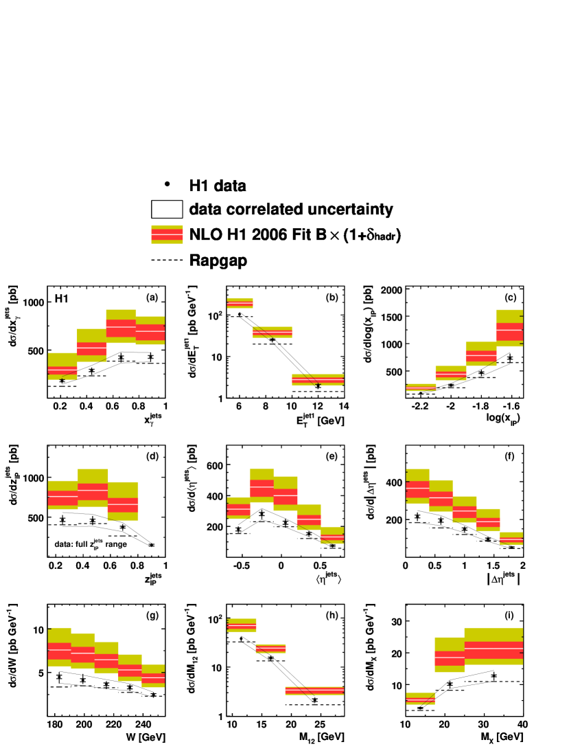
Figure 2: Diffractive dijet photoproduction cross sections differential in (a) $x_{\gamma}^{\rm jets}$, (b) $E_{T}^{\rm jet1}$, (c) $\log x_{{I\!\!P}}$, (d) $z_{{I\!\!P}}^{\rm jets}$, (e) $\left<\eta^{\rm jets}\right>$, (f) $\left|\Delta\eta^{\rm jets}\right|$, (g) $W$, (h) $M_{12}$ and (i) $M_{X}$. The data points are shown with inner error bars corresponding to statistical uncertainties and outer error bars representing statistical and uncorrelated systematic uncertainties added in quadrature. The correlated systematic errors are indicated by the open bands between the two solid black lines. The white lines show NLO QCD calculations obtained using the FR framework [26, 32, 33] and the H1 2006 Fit B DPDFs, corrected for hadronisation effects. The dark bands around the theoretical predictions indicate the result of propagating the uncertainties on the Fit B DPDFs to the NLO calculation. The light bands show this DPDF uncertainty added in quadrature with the effect on the calculation of varying $\mu_{R}$ and $\mu_{F}$ by factors of 0.5 and 2.0. In all figures, the predictions of the RAPGAP MC model are also shown.

$\displaystyle x^{\rm jets}_{\gamma}$			$\displaystyle\mbox{d}\sigma/\mbox{d}x^{\rm jets}_{\gamma}\,\,[\mbox{pb}]$	$\displaystyle\delta_{\mbox{\tiny stat}}$	$\displaystyle\delta_{\mbox{\tiny uncorr}}$	$\displaystyle\delta_{\mbox{\tiny corr}}$	$\displaystyle 1+\delta_{\mbox{\tiny hadr}}$
$\displaystyle{\scriptstyle 0.1}$	​​​​$\displaystyle{\scriptstyle\div}$​​​​	$\displaystyle{\scriptstyle 0.325}$	$\displaystyle{\scriptstyle 181}$	$\displaystyle{\scriptstyle\pm 12}$	$\displaystyle{\scriptstyle+19/\!-\!24}$	$\displaystyle{\scriptstyle+42/\!-\!36}$	$\displaystyle{\scriptstyle 0.71}$
$\displaystyle{\scriptstyle 0.325}$	​​​​$\displaystyle{\scriptstyle\div}$​​​​	$\displaystyle{\scriptstyle 0.55}$	$\displaystyle{\scriptstyle 287}$	$\displaystyle{\scriptstyle\pm 12}$	$\displaystyle{\scriptstyle+29/\!-\!42}$	$\displaystyle{\scriptstyle+52/\!-\!47}$	$\displaystyle{\scriptstyle 0.78}$
$\displaystyle{\scriptstyle 0.55}$	​​​​$\displaystyle{\scriptstyle\div}$​​​​	$\displaystyle{\scriptstyle 0.775}$	$\displaystyle{\scriptstyle 423}$	$\displaystyle{\scriptstyle\pm 15}$	$\displaystyle{\scriptstyle+45/\!-\!49}$	$\displaystyle{\scriptstyle+57/\!-\!58}$	$\displaystyle{\scriptstyle 1.2}$
$\displaystyle{\scriptstyle 0.775}$	​​​​$\displaystyle{\scriptstyle\div}$​​​​	$\displaystyle{\scriptstyle 1}$	$\displaystyle{\scriptstyle 428}$	$\displaystyle{\scriptstyle\pm 14}$	$\displaystyle{\scriptstyle+44/\!-\!50}$	$\displaystyle{\scriptstyle+45/\!-\!48}$	$\displaystyle{\scriptstyle 0.71}$
$\displaystyle E_{T}^{\rm jet1}\,\,[\!~{}\mbox{GeV}]$			$\displaystyle\mbox{d}\sigma/\mbox{d}E_{T}^{\rm jet1}\,\,[\!~{}\mbox{pb}~{}\mbox{GeV}^{-1}]$	$\displaystyle\delta_{\mbox{\tiny stat}}$	$\displaystyle\delta_{\mbox{\tiny uncorr}}$	$\displaystyle\delta_{\mbox{\tiny corr}}$	$\displaystyle 1+\delta_{\mbox{\tiny hadr}}$
$\displaystyle{\scriptstyle 5}$	​​​​$\displaystyle{\scriptstyle\div}$​​​​	$\displaystyle{\scriptstyle 7}$	$\displaystyle{\scriptstyle 104}$	$\displaystyle{\scriptstyle\pm 3}$	$\displaystyle{\scriptstyle+9.7/\!-\!12}$	$\displaystyle{\scriptstyle+13/\!-\!14}$	$\displaystyle{\scriptstyle 0.82}$
$\displaystyle{\scriptstyle 7}$	​​​​$\displaystyle{\scriptstyle\div}$​​​​	$\displaystyle{\scriptstyle 10}$	$\displaystyle{\scriptstyle 25.3}$	$\displaystyle{\scriptstyle\pm 0.9}$	$\displaystyle{\scriptstyle+2.5/\!-\!3.2}$	$\displaystyle{\scriptstyle+3.7/\!-\!3.5}$	$\displaystyle{\scriptstyle 0.94}$
$\displaystyle{\scriptstyle 10}$	​​​​$\displaystyle{\scriptstyle\div}$​​​​	$\displaystyle{\scriptstyle 14}$	$\displaystyle{\scriptstyle 1.96}$	$\displaystyle{\scriptstyle\pm 0.16}$	$\displaystyle{\scriptstyle+0.29/\!-\!0.25}$	$\displaystyle{\scriptstyle+0.36/\!-\!0.36}$	$\displaystyle{\scriptstyle 0.90}$
$\displaystyle\mbox{log}(x_{{I\!\!P}})$			$\displaystyle\mbox{d}\sigma/\mbox{d}\mbox{log}(x_{{I\!\!P}})\,\,[\mbox{pb}]$	$\displaystyle\delta_{\mbox{\tiny stat}}$	$\displaystyle\delta_{\mbox{\tiny uncorr}}$	$\displaystyle\delta_{\mbox{\tiny corr}}$	$\displaystyle 1+\delta_{\mbox{\tiny hadr}}$
$\displaystyle{\scriptstyle-2.3}$	​​​​$\displaystyle{\scriptstyle\div}$​​​​	$\displaystyle{\scriptstyle-2.1}$	$\displaystyle{\scriptstyle 92}$	$\displaystyle{\scriptstyle\pm 7}$	$\displaystyle{\scriptstyle+8/\!-\!11}$	$\displaystyle{\scriptstyle+13/\!-\!14}$	$\displaystyle{\scriptstyle 0.93}$
$\displaystyle{\scriptstyle-2.1}$	​​​​$\displaystyle{\scriptstyle\div}$​​​​	$\displaystyle{\scriptstyle-1.9}$	$\displaystyle{\scriptstyle 238}$	$\displaystyle{\scriptstyle\pm 13}$	$\displaystyle{\scriptstyle+22/\!-\!30}$	$\displaystyle{\scriptstyle+31/\!-\!27}$	$\displaystyle{\scriptstyle 0.90}$
$\displaystyle{\scriptstyle-1.9}$	​​​​$\displaystyle{\scriptstyle\div}$​​​​	$\displaystyle{\scriptstyle-1.7}$	$\displaystyle{\scriptstyle 466}$	$\displaystyle{\scriptstyle\pm 16}$	$\displaystyle{\scriptstyle+50/\!-\!60}$	$\displaystyle{\scriptstyle+60/\!-\!61}$	$\displaystyle{\scriptstyle 0.84}$
$\displaystyle{\scriptstyle-1.7}$	​​​​$\displaystyle{\scriptstyle\div}$​​​​	$\displaystyle{\scriptstyle-1.523}$	$\displaystyle{\scriptstyle 734}$	$\displaystyle{\scriptstyle\pm 23}$	$\displaystyle{\scriptstyle+78/\!-\!85}$	$\displaystyle{\scriptstyle+11/\!-\!10}$	$\displaystyle{\scriptstyle 0.82}$
$\displaystyle z^{\rm jets}_{{I\!\!P}}$			$\displaystyle\mbox{d}\sigma/\mbox{d}z^{\rm jets}_{{I\!\!P}}\,\,[\mbox{pb}]$	$\displaystyle\delta_{\mbox{\tiny stat}}$	$\displaystyle\delta_{\mbox{\tiny uncorr}}$	$\displaystyle\delta_{\mbox{\tiny corr}}$	$\displaystyle 1+\delta_{\mbox{\tiny hadr}}$
$\displaystyle{\scriptstyle 0.14}$	​​​​$\displaystyle{\scriptstyle\div}$​​​​	$\displaystyle{\scriptstyle 0.36}$	$\displaystyle{\scriptstyle 471}$	$\displaystyle{\scriptstyle\pm 19}$	$\displaystyle{\scriptstyle+54/\!-\!66}$	$\displaystyle{\scriptstyle+68/\!-\!67}$	$\displaystyle{\scriptstyle 0.79}$
$\displaystyle{\scriptstyle 0.36}$	​​​​$\displaystyle{\scriptstyle\div}$​​​​	$\displaystyle{\scriptstyle 0.58}$	$\displaystyle{\scriptstyle 460}$	$\displaystyle{\scriptstyle\pm 15}$	$\displaystyle{\scriptstyle+54/\!-\!63}$	$\displaystyle{\scriptstyle+60/\!-\!59}$	$\displaystyle{\scriptstyle 0.86}$
$\displaystyle{\scriptstyle 0.58}$	​​​​$\displaystyle{\scriptstyle\div}$​​​​	$\displaystyle{\scriptstyle 0.8}$	$\displaystyle{\scriptstyle 374}$	$\displaystyle{\scriptstyle\pm 12}$	$\displaystyle{\scriptstyle+42/\!-\!47}$	$\displaystyle{\scriptstyle+49/\!-\!49}$	$\displaystyle{\scriptstyle 0.92}$
$\displaystyle{\scriptstyle 0.8}$	​​​​$\displaystyle{\scriptstyle\div}$​​​​	$\displaystyle{\scriptstyle 1}$	$\displaystyle{\scriptstyle 151}$	$\displaystyle{\scriptstyle\pm 12}$	$\displaystyle{\scriptstyle+19/\!-\!18}$	$\displaystyle{\scriptstyle+21/\!-\!22}$	$\displaystyle-$
$\displaystyle\left<\eta^{\rm jets}\right>$			$\displaystyle\mbox{d}\sigma/\mbox{d}\left<\eta^{\rm jets}\right>\,\,[\mbox{pb}]$	$\displaystyle\delta_{\mbox{\tiny stat}}$	$\displaystyle\delta_{\mbox{\tiny uncorr}}$	$\displaystyle\delta_{\mbox{\tiny corr}}$	$\displaystyle 1+\delta_{\mbox{\tiny hadr}}$
$\displaystyle{\scriptstyle-0.7}$	​​​​$\displaystyle{\scriptstyle\div}$​​​​	$\displaystyle{\scriptstyle-0.4}$	$\displaystyle{\scriptstyle 181}$	$\displaystyle{\scriptstyle\pm 1}$	$\displaystyle{\scriptstyle+15/\!-\!20}$	$\displaystyle{\scriptstyle+29/\!-\!29}$	$\displaystyle{\scriptstyle 0.79}$
$\displaystyle{\scriptstyle-0.4}$	​​​​$\displaystyle{\scriptstyle\div}$​​​​	$\displaystyle{\scriptstyle-0.1}$	$\displaystyle{\scriptstyle 280}$	$\displaystyle{\scriptstyle\pm 10}$	$\displaystyle{\scriptstyle+26/\!-\!31}$	$\displaystyle{\scriptstyle+36/\!-\!37}$	$\displaystyle{\scriptstyle 0.93}$
$\displaystyle{\scriptstyle-0.1}$	​​​​$\displaystyle{\scriptstyle\div}$​​​​	$\displaystyle{\scriptstyle 0.2}$	$\displaystyle{\scriptstyle 224}$	$\displaystyle{\scriptstyle\pm 10}$	$\displaystyle{\scriptstyle+24/\!-\!30}$	$\displaystyle{\scriptstyle+27/\!-\!28}$	$\displaystyle{\scriptstyle 0.93}$
$\displaystyle{\scriptstyle 0.2}$	​​​​$\displaystyle{\scriptstyle\div}$​​​​	$\displaystyle{\scriptstyle 0.5}$	$\displaystyle{\scriptstyle 153}$	$\displaystyle{\scriptstyle\pm 7}$	$\displaystyle{\scriptstyle+17/\!-\!18}$	$\displaystyle{\scriptstyle+20/\!-\!19}$	$\displaystyle{\scriptstyle 0.80}$
$\displaystyle{\scriptstyle 0.5}$	​​​​$\displaystyle{\scriptstyle\div}$​​​​	$\displaystyle{\scriptstyle 0.8}$	$\displaystyle{\scriptstyle 75}$	$\displaystyle{\scriptstyle\pm 5}$	$\displaystyle{\scriptstyle+8/\!-\!10}$	$\displaystyle{\scriptstyle+10/\!-\!10}$	$\displaystyle{\scriptstyle 0.75}$
$\displaystyle\left|\Delta\eta^{\rm jets}\right|$			$\displaystyle\mbox{d}\sigma/\mbox{d}\left|\Delta\eta^{\rm jets}\right|\,\,[\mbox{pb}]$	$\displaystyle\delta_{\mbox{\tiny stat}}$	$\displaystyle\delta_{\mbox{\tiny uncorr}}$	$\displaystyle\delta_{\mbox{\tiny corr}}$	$\displaystyle 1+\delta_{\mbox{\tiny hadr}}$
$\displaystyle{\scriptstyle 0}$	​​​​$\displaystyle{\scriptstyle\div}$​​​​	$\displaystyle{\scriptstyle 0.4}$	$\displaystyle{\scriptstyle 216}$	$\displaystyle{\scriptstyle\pm 8}$	$\displaystyle{\scriptstyle+21/\!-\!22}$	$\displaystyle{\scriptstyle+32/\!-\!31}$	$\displaystyle{\scriptstyle 0.81}$
$\displaystyle{\scriptstyle 0.4}$	​​​​$\displaystyle{\scriptstyle\div}$​​​​	$\displaystyle{\scriptstyle 0.8}$	$\displaystyle{\scriptstyle 195}$	$\displaystyle{\scriptstyle\pm 8}$	$\displaystyle{\scriptstyle+18/\!-\!22}$	$\displaystyle{\scriptstyle+26/\!-\!27}$	$\displaystyle{\scriptstyle 0.83}$
$\displaystyle{\scriptstyle 0.8}$	​​​​$\displaystyle{\scriptstyle\div}$​​​​	$\displaystyle{\scriptstyle 1.2}$	$\displaystyle{\scriptstyle 149}$	$\displaystyle{\scriptstyle\pm 6}$	$\displaystyle{\scriptstyle+12/\!-\!18}$	$\displaystyle{\scriptstyle+20/\!-\!19}$	$\displaystyle{\scriptstyle 0.85}$
$\displaystyle{\scriptstyle 1.2}$	​​​​$\displaystyle{\scriptstyle\div}$​​​​	$\displaystyle{\scriptstyle 1.6}$	$\displaystyle{\scriptstyle 96}$	$\displaystyle{\scriptstyle\pm 6}$	$\displaystyle{\scriptstyle+11/\!-\!14}$	$\displaystyle{\scriptstyle+13/\!-\!12}$	$\displaystyle{\scriptstyle 0.93}$
$\displaystyle{\scriptstyle 1.6}$	​​​​$\displaystyle{\scriptstyle\div}$​​​​	$\displaystyle{\scriptstyle 2}$	$\displaystyle{\scriptstyle 51.7}$	$\displaystyle{\scriptstyle\pm 3.5}$	$\displaystyle{\scriptstyle+5.5/\!-\!6.2}$	$\displaystyle{\scriptstyle+6.8/\!-\!6.9}$	$\displaystyle{\scriptstyle 0.80}$
$\displaystyle W\,\,[\!~{}\mbox{GeV}]$			$\displaystyle\mbox{d}\sigma/\mbox{d}W\,\,[\!~{}\mbox{pb}~{}\mbox{GeV}^{-1}]$	$\displaystyle\delta_{\mbox{\tiny stat}}$	$\displaystyle\delta_{\mbox{\tiny uncorr}}$	$\displaystyle\delta_{\mbox{\tiny corr}}$	$\displaystyle 1+\delta_{\mbox{\tiny hadr}}$
$\displaystyle{\scriptstyle 175}$	​​​​$\displaystyle{\scriptstyle\div}$​​​​	$\displaystyle{\scriptstyle 191}$	$\displaystyle{\scriptstyle 4.50}$	$\displaystyle{\scriptstyle\pm 0.21}$	$\displaystyle{\scriptstyle+0.51/\!-\!0.70}$	$\displaystyle{\scriptstyle+0.63/\!-\!0.71}$	$\displaystyle{\scriptstyle 0.80}$
$\displaystyle{\scriptstyle 191}$	​​​​$\displaystyle{\scriptstyle\div}$​​​​	$\displaystyle{\scriptstyle 207}$	$\displaystyle{\scriptstyle 4.14}$	$\displaystyle{\scriptstyle\pm 0.17}$	$\displaystyle{\scriptstyle+0.70/\!-\!0.40}$	$\displaystyle{\scriptstyle+0.58/\!-\!0.62}$	$\displaystyle{\scriptstyle 0.84}$
$\displaystyle{\scriptstyle 207}$	​​​​$\displaystyle{\scriptstyle\div}$​​​​	$\displaystyle{\scriptstyle 223}$	$\displaystyle{\scriptstyle 3.67}$	$\displaystyle{\scriptstyle\pm 0.14}$	$\displaystyle{\scriptstyle+0.31/\!-\!0.53}$	$\displaystyle{\scriptstyle+0.52/\!-\!0.53}$	$\displaystyle{\scriptstyle 0.88}$
$\displaystyle{\scriptstyle 223}$	​​​​$\displaystyle{\scriptstyle\div}$​​​​	$\displaystyle{\scriptstyle 239}$	$\displaystyle{\scriptstyle 3.30}$	$\displaystyle{\scriptstyle\pm 0.16}$	$\displaystyle{\scriptstyle+0.31/\!-\!0.37}$	$\displaystyle{\scriptstyle+0.43/\!-\!0.38}$	$\displaystyle{\scriptstyle 0.86}$
$\displaystyle{\scriptstyle 239}$	​​​​$\displaystyle{\scriptstyle\div}$​​​​	$\displaystyle{\scriptstyle 255}$	$\displaystyle{\scriptstyle 2.46}$	$\displaystyle{\scriptstyle\pm 0.14}$	$\displaystyle{\scriptstyle+0.25/\!-\!0.29}$	$\displaystyle{\scriptstyle+0.31/\!-\!0.28}$	$\displaystyle{\scriptstyle 0.85}$
$\displaystyle M_{12}\,\,[\!~{}\mbox{GeV}]$			$\displaystyle\mbox{d}\sigma/\mbox{d}M_{12}\,\,[\!~{}\mbox{pb}~{}\mbox{GeV}^{-1}]$	$\displaystyle\delta_{\mbox{\tiny stat}}$	$\displaystyle\delta_{\mbox{\tiny uncorr}}$	$\displaystyle\delta_{\mbox{\tiny corr}}$	$\displaystyle 1+\delta_{\mbox{\tiny hadr}}$
$\displaystyle{\scriptstyle 9}$	​​​​$\displaystyle{\scriptstyle\div}$​​​​	$\displaystyle{\scriptstyle 14}$	$\displaystyle{\scriptstyle 38.2}$	$\displaystyle{\scriptstyle\pm 1.0}$	$\displaystyle{\scriptstyle+3.3/\!-\!4.3}$	$\displaystyle{\scriptstyle+5.1/\!-\!5.0}$	$\displaystyle{\scriptstyle 0.82}$
$\displaystyle{\scriptstyle 14}$	​​​​$\displaystyle{\scriptstyle\div}$​​​​	$\displaystyle{\scriptstyle 19}$	$\displaystyle{\scriptstyle 15.4}$	$\displaystyle{\scriptstyle\pm 0.6}$	$\displaystyle{\scriptstyle+1.7/\!-\!2.0}$	$\displaystyle{\scriptstyle+1.9/\!-\!2.0}$	$\displaystyle{\scriptstyle 0.88}$
$\displaystyle{\scriptstyle 19}$	​​​​$\displaystyle{\scriptstyle\div}$​​​​	$\displaystyle{\scriptstyle 29}$	$\displaystyle{\scriptstyle 2.12}$	$\displaystyle{\scriptstyle\pm 0.14}$	$\displaystyle{\scriptstyle+0.26/\!-\!0.23}$	$\displaystyle{\scriptstyle+0.43/\!-\!0.35}$	$\displaystyle{\scriptstyle 0.97}$
$\displaystyle M_{X}\,\,[\!~{}\mbox{GeV}]$			$\displaystyle\mbox{d}\sigma/\mbox{d}M_{X}\,\,[\!~{}\mbox{pb}~{}\mbox{GeV}^{-1}]$	$\displaystyle\delta_{\mbox{\tiny stat}}$	$\displaystyle\delta_{\mbox{\tiny uncorr}}$	$\displaystyle\delta_{\mbox{\tiny corr}}$	$\displaystyle 1+\delta_{\mbox{\tiny hadr}}$
$\displaystyle{\scriptstyle 10}$	​​​​$\displaystyle{\scriptstyle\div}$​​​​	$\displaystyle{\scriptstyle 17.5}$	$\displaystyle{\scriptstyle 2.61}$	$\displaystyle{\scriptstyle\pm 0.20}$	$\displaystyle{\scriptstyle+0.28/\!-\!0.30}$	$\displaystyle{\scriptstyle\pm 0.45}$	$\displaystyle{\scriptstyle 0.94}$
$\displaystyle{\scriptstyle 17.5}$	​​​​$\displaystyle{\scriptstyle\div}$​​​​	$\displaystyle{\scriptstyle 25}$	$\displaystyle{\scriptstyle 10.1}$	$\displaystyle{\scriptstyle\pm 0.4}$	$\displaystyle{\scriptstyle+1.0/\!-\!1.3}$	$\displaystyle{\scriptstyle\pm 1.3}$	$\displaystyle{\scriptstyle 0.87}$
$\displaystyle{\scriptstyle 25}$	​​​​$\displaystyle{\scriptstyle\div}$​​​​	$\displaystyle{\scriptstyle 40}$	$\displaystyle{\scriptstyle 12.8}$	$\displaystyle{\scriptstyle\pm 0.3}$	$\displaystyle{\scriptstyle+1.2/\!-\!1.5}$	$\displaystyle{\scriptstyle\pm 1.7}$	$\displaystyle{\scriptstyle 0.83}$

Table 2: Bin averaged hadron level differential cross sections for diffractive dijet photoproduction. For each data point, the absolute statistical, uncorrelated and correlated systematic uncertainties and the hadronisation correction factors applied to the NLO calculations are given as $\displaystyle\delta_{\mbox{\tiny stat}}$, $\displaystyle\delta_{\mbox{\tiny uncorr}}$ and $\displaystyle\delta_{\mbox{\tiny corr}}$ and $\displaystyle 1+\delta_{\mbox{\tiny hadr}}$, respectively.

$\displaystyle x^{\rm jets}_{\gamma}$			$\displaystyle\mbox{data}/\mbox{theory}$	$\displaystyle\delta_{\mbox{\tiny stat}}$	$\displaystyle\delta_{\mbox{\tiny uncorr}}$	$\displaystyle\delta_{\mbox{\tiny corr}}$	$\displaystyle\delta_{\mbox{\tiny DPDF}}$	$\displaystyle\delta_{\mbox{\tiny scal}}$
$\displaystyle{\scriptstyle 0.1}$	​​​​$\displaystyle{\scriptstyle\div}$​​​​	$\displaystyle{\scriptstyle 0.325}$	$\displaystyle{\scriptstyle 0.62}$	$\displaystyle{\scriptstyle\pm 0.04}$	$\displaystyle{\scriptstyle+0.06/-0.08}$	$\displaystyle{\scriptstyle+0.14/-0.12}$	$\displaystyle{\scriptstyle+0.12/-0.06}$	$\displaystyle{\scriptstyle+0.28/-0.23}$
$\displaystyle{\scriptstyle 0.325}$	​​​​$\displaystyle{\scriptstyle\div}$​​​​	$\displaystyle{\scriptstyle 0.55}$	$\displaystyle{\scriptstyle 0.55}$	$\displaystyle{\scriptstyle\pm 0.02}$	$\displaystyle{\scriptstyle+0.06/-0.08}$	$\displaystyle{\scriptstyle+0.01/-0.09}$	$\displaystyle{\scriptstyle+0.09/-0.05}$	$\displaystyle{\scriptstyle+0.16/-0.15}$
$\displaystyle{\scriptstyle 0.55}$	​​​​$\displaystyle{\scriptstyle\div}$​​​​	$\displaystyle{\scriptstyle 0.775}$	$\displaystyle{\scriptstyle 0.57}$	$\displaystyle{\scriptstyle\pm 0.02}$	$\displaystyle{\scriptstyle+0.06/-0.07}$	$\displaystyle{\scriptstyle+0.08/-0.08}$	$\displaystyle{\scriptstyle+0.09/-0.05}$	$\displaystyle{\scriptstyle+0.11/-0.10}$
$\displaystyle{\scriptstyle 0.775}$	​​​​$\displaystyle{\scriptstyle\div}$​​​​	$\displaystyle{\scriptstyle 1}$	$\displaystyle{\scriptstyle 0.62}$	$\displaystyle{\scriptstyle\pm 0.02}$	$\displaystyle{\scriptstyle+0.06/-0.07}$	$\displaystyle{\scriptstyle+0.07/-0.07}$	$\displaystyle{\scriptstyle+0.10/-0.06}$	$\displaystyle{\scriptstyle+0.10/-0.01}$
$\displaystyle E_{T}^{\rm jet1}\,\,[\!~{}\mbox{GeV}]$			$\displaystyle\mbox{data}/\mbox{theory}$	$\displaystyle\delta_{\mbox{\tiny stat}}$	$\displaystyle\delta_{\mbox{\tiny uncorr}}$	$\displaystyle\delta_{\mbox{\tiny corr}}$	$\displaystyle\delta_{\mbox{\tiny DPDF}}$	$\displaystyle\delta_{\mbox{\tiny scal}}$
$\displaystyle{\scriptstyle 5}$	​​​​$\displaystyle{\scriptstyle\div}$​​​​	$\displaystyle{\scriptstyle 7}$	$\displaystyle{\scriptstyle 0.54}$	$\displaystyle{\scriptstyle\pm 0.01}$	$\displaystyle{\scriptstyle+0.05/-0.06}$	$\displaystyle{\scriptstyle+0.07/-0.07}$	$\displaystyle{\scriptstyle+0.09/-0.05}$	$\displaystyle{\scriptstyle+0.13/-0.12}$
$\displaystyle{\scriptstyle 7}$	​​​​$\displaystyle{\scriptstyle\div}$​​​​	$\displaystyle{\scriptstyle 10}$	$\displaystyle{\scriptstyle 0.66}$	$\displaystyle{\scriptstyle\pm 0.02}$	$\displaystyle{\scriptstyle+0.07/-0.08}$	$\displaystyle{\scriptstyle+0.10/-0.09}$	$\displaystyle{\scriptstyle+0.11/-0.07}$	$\displaystyle{\scriptstyle+0.18/-0.17}$
$\displaystyle{\scriptstyle 10}$	​​​​$\displaystyle{\scriptstyle\div}$​​​​	$\displaystyle{\scriptstyle 14}$	$\displaystyle{\scriptstyle 0.71}$	$\displaystyle{\scriptstyle\pm 0.06}$	$\displaystyle{\scriptstyle+0.10/-0.09}$	$\displaystyle{\scriptstyle+0.13/-0.13}$	$\displaystyle{\scriptstyle+0.13/-0.08}$	$\displaystyle{\scriptstyle+0.20/-0.18}$
$\displaystyle\mbox{log}(x_{{I\!\!P}})$			$\displaystyle\mbox{data}/\mbox{theory}$	$\displaystyle\delta_{\mbox{\tiny stat}}$	$\displaystyle\delta_{\mbox{\tiny uncorr}}$	$\displaystyle\delta_{\mbox{\tiny corr}}$	$\displaystyle\delta_{\mbox{\tiny DPDF}}$	$\displaystyle\delta_{\mbox{\tiny scal}}$
$\displaystyle{\scriptstyle-2.3}$	​​​​$\displaystyle{\scriptstyle\div}$​​​​	$\displaystyle{\scriptstyle-2.1}$	$\displaystyle{\scriptstyle 0.50}$	$\displaystyle{\scriptstyle\pm 0.08}$	$\displaystyle{\scriptstyle+0.04/-0.06}$	$\displaystyle{\scriptstyle+0.07/-0.08}$	$\displaystyle{\scriptstyle+0.07/-0.05}$	$\displaystyle{\scriptstyle+0.16/-0.14}$
$\displaystyle{\scriptstyle-2.1}$	​​​​$\displaystyle{\scriptstyle\div}$​​​​	$\displaystyle{\scriptstyle-1.9}$	$\displaystyle{\scriptstyle 0.54}$	$\displaystyle{\scriptstyle\pm 0.03}$	$\displaystyle{\scriptstyle+0.05/-0.07}$	$\displaystyle{\scriptstyle+0.07/-0.06}$	$\displaystyle{\scriptstyle+0.08/-0.05}$	$\displaystyle{\scriptstyle+0.15/-0.14}$
$\displaystyle{\scriptstyle-1.9}$	​​​​$\displaystyle{\scriptstyle\div}$​​​​	$\displaystyle{\scriptstyle-1.7}$	$\displaystyle{\scriptstyle 0.60}$	$\displaystyle{\scriptstyle\pm 0.02}$	$\displaystyle{\scriptstyle+0.06/-0.08}$	$\displaystyle{\scriptstyle+0.08/-0.08}$	$\displaystyle{\scriptstyle+0.10/-0.06}$	$\displaystyle{\scriptstyle+0.14/-0.14}$
$\displaystyle{\scriptstyle-1.7}$	​​​​$\displaystyle{\scriptstyle\div}$​​​​	$\displaystyle{\scriptstyle-1.523}$	$\displaystyle{\scriptstyle 0.59}$	$\displaystyle{\scriptstyle\pm 0.02}$	$\displaystyle{\scriptstyle+0.06/-0.07}$	$\displaystyle{\scriptstyle+0.09/-0.08}$	$\displaystyle{\scriptstyle+0.11/-0.06}$	$\displaystyle{\scriptstyle+0.13/-0.13}$
$\displaystyle z^{\rm jets}_{{I\!\!P}}$			$\displaystyle\mbox{data}/\mbox{theory}$	$\displaystyle\delta_{\mbox{\tiny stat}}$	$\displaystyle\delta_{\mbox{\tiny uncorr}}$	$\displaystyle\delta_{\mbox{\tiny corr}}$	$\displaystyle\delta_{\mbox{\tiny DPDF}}$	$\displaystyle\delta_{\mbox{\tiny scal}}$
$\displaystyle{\scriptstyle 0.14}$	​​​​$\displaystyle{\scriptstyle\div}$​​​​	$\displaystyle{\scriptstyle 0.36}$	$\displaystyle{\scriptstyle 0.62}$	$\displaystyle{\scriptstyle\pm 0.03}$	$\displaystyle{\scriptstyle+0.07/-0.09}$	$\displaystyle{\scriptstyle+0.09/-0.09}$	$\displaystyle{\scriptstyle+0.10/-0.06}$	$\displaystyle{\scriptstyle+0.11/-0.12}$
$\displaystyle{\scriptstyle 0.36}$	​​​​$\displaystyle{\scriptstyle\div}$​​​​	$\displaystyle{\scriptstyle 0.58}$	$\displaystyle{\scriptstyle 0.55}$	$\displaystyle{\scriptstyle\pm 0.02}$	$\displaystyle{\scriptstyle+0.07/-0.08}$	$\displaystyle{\scriptstyle+0.07/-0.07}$	$\displaystyle{\scriptstyle+0.09/-0.05}$	$\displaystyle{\scriptstyle+0.14/-0.13}$
$\displaystyle{\scriptstyle 0.58}$	​​​​$\displaystyle{\scriptstyle\div}$​​​​	$\displaystyle{\scriptstyle 0.8}$	$\displaystyle{\scriptstyle 0.57}$	$\displaystyle{\scriptstyle\pm 0.02}$	$\displaystyle{\scriptstyle+0.06/-0.07}$	$\displaystyle{\scriptstyle+0.07/-0.07}$	$\displaystyle{\scriptstyle+0.10/-0.06}$	$\displaystyle{\scriptstyle+0.20/-0.16}$
$\displaystyle\left<\eta^{\rm jets}\right>$			$\displaystyle\mbox{data}/\mbox{theory}$	$\displaystyle\delta_{\mbox{\tiny stat}}$	$\displaystyle\delta_{\mbox{\tiny uncorr}}$	$\displaystyle\delta_{\mbox{\tiny corr}}$	$\displaystyle\delta_{\mbox{\tiny DPDF}}$	$\displaystyle\delta_{\mbox{\tiny scal}}$
$\displaystyle{\scriptstyle-0.7}$	​​​​$\displaystyle{\scriptstyle\div}$​​​​	$\displaystyle{\scriptstyle-0.4}$	$\displaystyle{\scriptstyle 0.58}$	$\displaystyle{\scriptstyle\pm 0.03}$	$\displaystyle{\scriptstyle+0.05/-0.06}$	$\displaystyle{\scriptstyle+0.09/-0.09}$	$\displaystyle{\scriptstyle+0.09/-0.05}$	$\displaystyle{\scriptstyle+0.10/-0.10}$
$\displaystyle{\scriptstyle-0.4}$	​​​​$\displaystyle{\scriptstyle\div}$​​​​	$\displaystyle{\scriptstyle-0.1}$	$\displaystyle{\scriptstyle 0.62}$	$\displaystyle{\scriptstyle\pm 0.02}$	$\displaystyle{\scriptstyle+0.06/-0.07}$	$\displaystyle{\scriptstyle+0.08/-0.08}$	$\displaystyle{\scriptstyle+0.10/-0.06}$	$\displaystyle{\scriptstyle+0.12/-0.12}$
$\displaystyle{\scriptstyle-0.1}$	​​​​$\displaystyle{\scriptstyle\div}$​​​​	$\displaystyle{\scriptstyle 0.2}$	$\displaystyle{\scriptstyle 0.56}$	$\displaystyle{\scriptstyle\pm 0.02}$	$\displaystyle{\scriptstyle+0.06/-0.07}$	$\displaystyle{\scriptstyle+0.07/-0.07}$	$\displaystyle{\scriptstyle+0.10/-0.05}$	$\displaystyle{\scriptstyle+0.14/-0.12}$
$\displaystyle{\scriptstyle 0.2}$	​​​​$\displaystyle{\scriptstyle\div}$​​​​	$\displaystyle{\scriptstyle 0.5}$	$\displaystyle{\scriptstyle 0.62}$	$\displaystyle{\scriptstyle\pm 0.03}$	$\displaystyle{\scriptstyle+0.07/-0.07}$	$\displaystyle{\scriptstyle+0.08/-0.08}$	$\displaystyle{\scriptstyle+0.11/-0.06}$	$\displaystyle{\scriptstyle+0.19/-0.17}$
$\displaystyle{\scriptstyle 0.5}$	​​​​$\displaystyle{\scriptstyle\div}$​​​​	$\displaystyle{\scriptstyle 0.8}$	$\displaystyle{\scriptstyle 0.57}$	$\displaystyle{\scriptstyle\pm 0.04}$	$\displaystyle{\scriptstyle+0.06/-0.08}$	$\displaystyle{\scriptstyle+0.08/-0.07}$	$\displaystyle{\scriptstyle+0.11/-0.06}$	$\displaystyle{\scriptstyle+0.23/-0.18}$
$\displaystyle\left|\Delta\eta^{\rm jets}\right|$			$\displaystyle\mbox{data}/\mbox{theory}$	$\displaystyle\delta_{\mbox{\tiny stat}}$	$\displaystyle\delta_{\mbox{\tiny uncorr}}$	$\displaystyle\delta_{\mbox{\tiny corr}}$	$\displaystyle\delta_{\mbox{\tiny DPDF}}$	$\displaystyle\delta_{\mbox{\tiny scal}}$
$\displaystyle{\scriptstyle 0}$	​​​​$\displaystyle{\scriptstyle\div}$​​​​	$\displaystyle{\scriptstyle 0.4}$	$\displaystyle{\scriptstyle 0.59}$	$\displaystyle{\scriptstyle\pm 0.02}$	$\displaystyle{\scriptstyle+0.06/-0.06}$	$\displaystyle{\scriptstyle+0.09/-0.09}$	$\displaystyle{\scriptstyle+0.09/-0.06}$	$\displaystyle{\scriptstyle+0.12/-0.12}$
$\displaystyle{\scriptstyle 0.4}$	​​​​$\displaystyle{\scriptstyle\div}$​​​​	$\displaystyle{\scriptstyle 0.8}$	$\displaystyle{\scriptstyle 0.62}$	$\displaystyle{\scriptstyle\pm 0.03}$	$\displaystyle{\scriptstyle+0.06/-0.07}$	$\displaystyle{\scriptstyle+0.08/-0.09}$	$\displaystyle{\scriptstyle+0.10/-0.06}$	$\displaystyle{\scriptstyle+0.14/-0.13}$
$\displaystyle{\scriptstyle 0.8}$	​​​​$\displaystyle{\scriptstyle\div}$​​​​	$\displaystyle{\scriptstyle 1.2}$	$\displaystyle{\scriptstyle 0.61}$	$\displaystyle{\scriptstyle\pm 0.03}$	$\displaystyle{\scriptstyle+0.05/-0.07}$	$\displaystyle{\scriptstyle+0.08/-0.08}$	$\displaystyle{\scriptstyle+0.11/-0.06}$	$\displaystyle{\scriptstyle+0.15/-0.14}$
$\displaystyle{\scriptstyle 1.2}$	​​​​$\displaystyle{\scriptstyle\div}$​​​​	$\displaystyle{\scriptstyle 1.6}$	$\displaystyle{\scriptstyle 0.51}$	$\displaystyle{\scriptstyle\pm 0.03}$	$\displaystyle{\scriptstyle+0.06/-0.07}$	$\displaystyle{\scriptstyle+0.07/-0.07}$	$\displaystyle{\scriptstyle+0.09/-0.05}$	$\displaystyle{\scriptstyle+0.14/-0.13}$
$\displaystyle{\scriptstyle 1.6}$	​​​​$\displaystyle{\scriptstyle\div}$​​​​	$\displaystyle{\scriptstyle 2}$	$\displaystyle{\scriptstyle 0.55}$	$\displaystyle{\scriptstyle\pm 0.04}$	$\displaystyle{\scriptstyle+0.06/-0.07}$	$\displaystyle{\scriptstyle+0.07/-0.07}$	$\displaystyle{\scriptstyle+0.10/-0.05}$	$\displaystyle{\scriptstyle+0.17/-0.16}$
$\displaystyle W\,\,[\!~{}\mbox{GeV}]$			$\displaystyle\mbox{data}/\mbox{theory}$	$\displaystyle\delta_{\mbox{\tiny stat}}$	$\displaystyle\delta_{\mbox{\tiny uncorr}}$	$\displaystyle\delta_{\mbox{\tiny corr}}$	$\displaystyle\delta_{\mbox{\tiny DPDF}}$	$\displaystyle\delta_{\mbox{\tiny scal}}$
$\displaystyle{\scriptstyle 175}$	​​​​$\displaystyle{\scriptstyle\div}$​​​​	$\displaystyle{\scriptstyle 191}$	$\displaystyle{\scriptstyle 0.59}$	$\displaystyle{\scriptstyle\pm 0.03}$	$\displaystyle{\scriptstyle+0.07/-0.09}$	$\displaystyle{\scriptstyle+0.08/-0.09}$	$\displaystyle{\scriptstyle+0.10/-0.06}$	$\displaystyle{\scriptstyle+0.15/-0.14}$
$\displaystyle{\scriptstyle 191}$	​​​​$\displaystyle{\scriptstyle\div}$​​​​	$\displaystyle{\scriptstyle 207}$	$\displaystyle{\scriptstyle 0.57}$	$\displaystyle{\scriptstyle\pm 0.02}$	$\displaystyle{\scriptstyle+0.10/-0.06}$	$\displaystyle{\scriptstyle+0.08/-0.09}$	$\displaystyle{\scriptstyle+0.10/-0.05}$	$\displaystyle{\scriptstyle+0.14/-0.13}$
$\displaystyle{\scriptstyle 207}$	​​​​$\displaystyle{\scriptstyle\div}$​​​​	$\displaystyle{\scriptstyle 223}$	$\displaystyle{\scriptstyle 0.57}$	$\displaystyle{\scriptstyle\pm 0.02}$	$\displaystyle{\scriptstyle+0.05/-0.08}$	$\displaystyle{\scriptstyle+0.08/-0.08}$	$\displaystyle{\scriptstyle+0.10/-0.05}$	$\displaystyle{\scriptstyle+0.13/-0.13}$
$\displaystyle{\scriptstyle 223}$	​​​​$\displaystyle{\scriptstyle\div}$​​​​	$\displaystyle{\scriptstyle 239}$	$\displaystyle{\scriptstyle 0.62}$	$\displaystyle{\scriptstyle\pm 0.03}$	$\displaystyle{\scriptstyle+0.06/-0.07}$	$\displaystyle{\scriptstyle+0.08/-0.07}$	$\displaystyle{\scriptstyle+0.10/-0.06}$	$\displaystyle{\scriptstyle+0.15/-0.14}$
$\displaystyle{\scriptstyle 239}$	​​​​$\displaystyle{\scriptstyle\div}$​​​​	$\displaystyle{\scriptstyle 255}$	$\displaystyle{\scriptstyle 0.56}$	$\displaystyle{\scriptstyle\pm 0.03}$	$\displaystyle{\scriptstyle+0.06/-0.07}$	$\displaystyle{\scriptstyle+0.07/-0.06}$	$\displaystyle{\scriptstyle+0.09/-0.06}$	$\displaystyle{\scriptstyle+0.14/-0.13}$
$\displaystyle M_{12}\,\,[\!~{}\mbox{GeV}]$			$\displaystyle\mbox{data}/\mbox{theory}$	$\displaystyle\delta_{\mbox{\tiny stat}}$	$\displaystyle\delta_{\mbox{\tiny uncorr}}$	$\displaystyle\delta_{\mbox{\tiny corr}}$	$\displaystyle\delta_{\mbox{\tiny DPDF}}$	$\displaystyle\delta_{\mbox{\tiny scal}}$
$\displaystyle{\scriptstyle 9}$	​​​​$\displaystyle{\scriptstyle\div}$​​​​	$\displaystyle{\scriptstyle 14}$	$\displaystyle{\scriptstyle 0.55}$	$\displaystyle{\scriptstyle\pm 0.01}$	$\displaystyle{\scriptstyle+0.05/-0.06}$	$\displaystyle{\scriptstyle+0.07/-0.07}$	$\displaystyle{\scriptstyle+0.09/-0.05}$	$\displaystyle{\scriptstyle+0.15/-0.15}$
$\displaystyle{\scriptstyle 14}$	​​​​$\displaystyle{\scriptstyle\div}$​​​​	$\displaystyle{\scriptstyle 19}$	$\displaystyle{\scriptstyle 0.63}$	$\displaystyle{\scriptstyle\pm 0.03}$	$\displaystyle{\scriptstyle+0.07/-0.08}$	$\displaystyle{\scriptstyle+0.08/-0.08}$	$\displaystyle{\scriptstyle+0.11/-0.06}$	$\displaystyle{\scriptstyle+0.10/-0.08}$
$\displaystyle{\scriptstyle 19}$	​​​​$\displaystyle{\scriptstyle\div}$​​​​	$\displaystyle{\scriptstyle 29}$	$\displaystyle{\scriptstyle 0.62}$	$\displaystyle{\scriptstyle\pm 0.04}$	$\displaystyle{\scriptstyle+0.08/-0.07}$	$\displaystyle{\scriptstyle+0.13/-0.10}$	$\displaystyle{\scriptstyle+0.11/-0.07}$	$\displaystyle{\scriptstyle+0.10/-0.05}$
$\displaystyle M_{X}\,\,[\!~{}\mbox{GeV}]$			$\displaystyle\mbox{data}/\mbox{theory}$	$\displaystyle\delta_{\mbox{\tiny stat}}$	$\displaystyle\delta_{\mbox{\tiny uncorr}}$	$\displaystyle\delta_{\mbox{\tiny corr}}$	$\displaystyle\delta_{\mbox{\tiny DPDF}}$	$\displaystyle\delta_{\mbox{\tiny scal}}$
$\displaystyle{\scriptstyle 10}$	​​​​$\displaystyle{\scriptstyle\div}$​​​​	$\displaystyle{\scriptstyle 17.5}$	$\displaystyle{\scriptstyle 0.51}$	$\displaystyle{\scriptstyle\pm 0.04}$	$\displaystyle{\scriptstyle+0.06/-0.06}$	$\displaystyle{\scriptstyle+0.09/-0.09}$	$\displaystyle{\scriptstyle+0.08/-0.05}$	$\displaystyle{\scriptstyle+0.17/-0.15}$
$\displaystyle{\scriptstyle 17.5}$	​​​​$\displaystyle{\scriptstyle\div}$​​​​	$\displaystyle{\scriptstyle 25}$	$\displaystyle{\scriptstyle 0.55}$	$\displaystyle{\scriptstyle\pm 0.02}$	$\displaystyle{\scriptstyle+0.05/-0.07}$	$\displaystyle{\scriptstyle+0.07/-0.07}$	$\displaystyle{\scriptstyle+0.09/-0.05}$	$\displaystyle{\scriptstyle+0.14/-0.13}$
$\displaystyle{\scriptstyle 25}$	​​​​$\displaystyle{\scriptstyle\div}$​​​​	$\displaystyle{\scriptstyle 40}$	$\displaystyle{\scriptstyle 0.60}$	$\displaystyle{\scriptstyle\pm 0.02}$	$\displaystyle{\scriptstyle+0.68/-0.07}$	$\displaystyle{\scriptstyle+0.08/-0.08}$	$\displaystyle{\scriptstyle+0.11/-0.06}$	$\displaystyle{\scriptstyle+0.14/-0.13}$

Table 3: Ratios of differential cross sections for diffractive dijet photoproduction to NLO QCD calculations obtained in the FR framework with the H1 2006 Fit B DPDFs, corrected for hadronisation. For each ratio point, the absolute statistical, uncorrelated and correlated systematic uncertainties from the data and the absolute DPDF and scale uncertainties from the theory are given as $\displaystyle\delta_{\mbox{\tiny stat}}$, $\displaystyle\delta_{\mbox{\tiny uncorr}}$, $\displaystyle\delta_{\mbox{\tiny corr}}$, $\displaystyle\delta_{\mbox{\tiny DPDF}}$ and $\displaystyle\delta_{\mbox{\tiny scal}}$, respectively.

$\displaystyle x^{\rm jets}_{\gamma}$			$\displaystyle E_{T}^{\rm jet1}[\mbox{GeV}]$	$\displaystyle\frac{\mbox{d}^{2}\sigma}{\mbox{d}x^{\rm jets}_{\gamma}\mbox{d}E_{T}^{\rm jet1}}\,\,[\mbox{pb}~{}\mbox{GeV}^{-1}]$	$\displaystyle\delta_{\mbox{\tiny stat}}$	$\displaystyle\delta_{\mbox{\tiny uncorr}}$	$\displaystyle\delta_{\mbox{\tiny corrr}}$	$\displaystyle 1+\delta_{\mbox{\tiny hadr}}$
$\displaystyle{\scriptstyle 0.1}$	​​​​$\displaystyle{\scriptstyle\div}$​​​​	$\displaystyle{\scriptstyle 0.75}$	$\displaystyle{\scriptstyle 5\,\,\div\,\,6.5}$	$\displaystyle{\scriptstyle 124}$	$\displaystyle{\scriptstyle\pm 4}$	$\displaystyle{\scriptstyle+12/-16}$	$\displaystyle{\scriptstyle+20/-19}$	$\displaystyle{\scriptstyle 0.84}$
$\displaystyle{\scriptstyle 0.75}$	​​​​$\displaystyle{\scriptstyle\div}$​​​​	$\displaystyle{\scriptstyle 1}$	$\displaystyle{\scriptstyle 5\,\,\div\,\,6.5}$	$\displaystyle{\scriptstyle 133}$	$\displaystyle{\scriptstyle\pm 7}$	$\displaystyle{\scriptstyle+13/-15}$	$\displaystyle{\scriptstyle+13/-14}$	$\displaystyle{\scriptstyle 0.72}$
$\displaystyle{\scriptstyle 0.1}$	​​​​$\displaystyle{\scriptstyle\div}$​​​​	$\displaystyle{\scriptstyle 0.75}$	$\displaystyle{\scriptstyle 6.5\,\,\div\,\,8.5}$	$\displaystyle{\scriptstyle 40.2}$	$\displaystyle{\scriptstyle\pm 1.9}$	$\displaystyle{\scriptstyle+4.6/-4.8}$	$\displaystyle{\scriptstyle+6.4/-6.5}$	$\displaystyle{\scriptstyle 0.99}$
$\displaystyle{\scriptstyle 0.75}$	​​​​$\displaystyle{\scriptstyle\div}$​​​​	$\displaystyle{\scriptstyle 1}$	$\displaystyle{\scriptstyle 6.5\,\,\div\,\,8.5}$	$\displaystyle{\scriptstyle 85}$	$\displaystyle{\scriptstyle\pm 4}$	$\displaystyle{\scriptstyle+9/-10}$	$\displaystyle{\scriptstyle+10/-10}$	$\displaystyle{\scriptstyle 0.84}$
$\displaystyle{\scriptstyle 0.1}$	​​​​$\displaystyle{\scriptstyle\div}$​​​​	$\displaystyle{\scriptstyle 0.75}$	$\displaystyle{\scriptstyle 8.5\,\,\div\,\,14}$	$\displaystyle{\scriptstyle 2.60}$	$\displaystyle{\scriptstyle\pm 0.25}$	$\displaystyle{\scriptstyle+0.30/-0.39}$	$\displaystyle{\scriptstyle+0.64/-0.45}$	$\displaystyle{\scriptstyle 1.0}$
$\displaystyle{\scriptstyle 0.75}$	​​​​$\displaystyle{\scriptstyle\div}$​​​​	$\displaystyle{\scriptstyle 1}$	$\displaystyle{\scriptstyle 8.5\,\,\div\,\,14}$	$\displaystyle{\scriptstyle 12.2}$	$\displaystyle{\scriptstyle\pm 0.7}$	$\displaystyle{\scriptstyle+1.3/-1.5}$	$\displaystyle{\scriptstyle+1.8/-1.8}$	$\displaystyle{\scriptstyle 0.88}$
$\displaystyle z^{\rm jets}_{{I\!\!P}}$			$\displaystyle x^{\rm jets}_{\gamma}$	$\displaystyle\frac{\mbox{d}^{2}\sigma}{\mbox{d}z^{\rm jets}_{{I\!\!P}}\mbox{d}x^{\rm jets}_{\gamma}}~{}[\mbox{pb}]$	$\displaystyle\delta_{\mbox{\tiny stat}}$	$\displaystyle\delta_{\mbox{\tiny uncorr}}$	$\displaystyle\delta_{\mbox{\tiny corrr}}$	$\displaystyle 1+\delta_{\mbox{\tiny hadr}}$
$\displaystyle{\scriptstyle 0.14}$	​​​​$\displaystyle{\scriptstyle\div}$​​​​	$\displaystyle{\scriptstyle 0.36}$	$\displaystyle{\scriptstyle 0.1\,\,\div\,\,0.75}$	$\displaystyle{\scriptstyle 403}$	$\displaystyle{\scriptstyle\pm 23}$	$\displaystyle{\scriptstyle+48/-59}$	$\displaystyle{\scriptstyle+76/-70}$	$\displaystyle{\scriptstyle 0.91}$
$\displaystyle{\scriptstyle 0.36}$	​​​​$\displaystyle{\scriptstyle\div}$​​​​	$\displaystyle{\scriptstyle 0.58}$	$\displaystyle{\scriptstyle 0.1\,\,\div\,\,0.75}$	$\displaystyle{\scriptstyle 477}$	$\displaystyle{\scriptstyle\pm 20}$	$\displaystyle{\scriptstyle+57/-71}$	$\displaystyle{\scriptstyle+79/-72}$	$\displaystyle{\scriptstyle 0.87}$
$\displaystyle{\scriptstyle 0.58}$	​​​​$\displaystyle{\scriptstyle\div}$​​​​	$\displaystyle{\scriptstyle 0.8}$	$\displaystyle{\scriptstyle 0.1\,\,\div\,\,0.75}$	$\displaystyle{\scriptstyle 386}$	$\displaystyle{\scriptstyle\pm 16}$	$\displaystyle{\scriptstyle+46/-53}$	$\displaystyle{\scriptstyle+59/-57}$	$\displaystyle{\scriptstyle 0.87}$
$\displaystyle{\scriptstyle 0.14}$	​​​​$\displaystyle{\scriptstyle\div}$​​​​	$\displaystyle{\scriptstyle 0.36}$	$\displaystyle{\scriptstyle 0.75\,\,\div\,\,1}$	$\displaystyle{\scriptstyle 846}$	$\displaystyle{\scriptstyle\pm 49}$	$\displaystyle{\scriptstyle+10/-12}$	$\displaystyle{\scriptstyle+10/-11}$	$\displaystyle{\scriptstyle 0.68}$
$\displaystyle{\scriptstyle 0.36}$	​​​​$\displaystyle{\scriptstyle\div}$​​​​	$\displaystyle{\scriptstyle 0.58}$	$\displaystyle{\scriptstyle 0.75\,\,\div\,\,1}$	$\displaystyle{\scriptstyle 605}$	$\displaystyle{\scriptstyle\pm 32}$	$\displaystyle{\scriptstyle+79/-81}$	$\displaystyle{\scriptstyle+61/-65}$	$\displaystyle{\scriptstyle 0.85}$
$\displaystyle{\scriptstyle 0.58}$	​​​​$\displaystyle{\scriptstyle\div}$​​​​	$\displaystyle{\scriptstyle 0.8}$	$\displaystyle{\scriptstyle 0.75\,\,\div\,\,1}$	$\displaystyle{\scriptstyle 489}$	$\displaystyle{\scriptstyle\pm 26}$	$\displaystyle{\scriptstyle+55/-58}$	$\displaystyle{\scriptstyle+49/-51}$	$\displaystyle{\scriptstyle 1.1}$

Table 4: Bin averaged hadron level double-differential cross sections for diffractive dijet photoproduction. For each data point, the absolute statistical, uncorrelated and correlated systematic uncertainties and the hadronisation correction factors applied to the NLO calculations are given as $\displaystyle\delta_{\mbox{\tiny stat}}$, $\displaystyle\delta_{\mbox{\tiny uncorr}}$ and $\displaystyle\delta_{\mbox{\tiny corr}}$ and $\displaystyle 1+\delta_{\mbox{\tiny hadr}}$, respectively.

$\displaystyle E_{T}^{\rm jet1}\,\,[\mbox{GeV}]$			$\displaystyle x^{\rm jets}_{\gamma}$	$\displaystyle\mbox{data}/\mbox{theory}$	$\displaystyle\delta_{\mbox{\tiny stat}}$	$\displaystyle\delta_{\mbox{\tiny uncorr}}$	$\displaystyle\delta_{\mbox{\tiny cororr}}$	$\displaystyle\delta_{\mbox{\tiny DPDF}}$	$\displaystyle\delta_{\mbox{\tiny scal}}$
$\displaystyle{\scriptstyle 5}$	​​​​$\displaystyle{\scriptstyle\div}$​​​​	$\displaystyle{\scriptstyle 6.5}$	$\displaystyle{\scriptstyle 0.1\,\,\div\,\,0.75}$	$\displaystyle{\scriptstyle 0.52}$	$\displaystyle{\scriptstyle\pm 0.02}$	$\displaystyle{\scriptstyle+0.05/-0.07}$	$\displaystyle{\scriptstyle+0.08/-0.08}$	$\displaystyle{\scriptstyle+0.09/-0.06}$	$\displaystyle{\scriptstyle+0.14/-0.13}$
$\displaystyle{\scriptstyle 6.5}$	​​​​$\displaystyle{\scriptstyle\div}$​​​​	$\displaystyle{\scriptstyle 8.5}$	$\displaystyle{\scriptstyle 0.1\,\,\div\,\,0.75}$	$\displaystyle{\scriptstyle 0.69}$	$\displaystyle{\scriptstyle\pm 0.03}$	$\displaystyle{\scriptstyle+0.08/-0.08}$	$\displaystyle{\scriptstyle+0.11/-0.11}$	$\displaystyle{\scriptstyle+0.12/-0.07}$	$\displaystyle{\scriptstyle+0.24/-0.21}$
$\displaystyle{\scriptstyle 8.5}$	​​​​$\displaystyle{\scriptstyle\div}$​​​​	$\displaystyle{\scriptstyle 14}$	$\displaystyle{\scriptstyle 0.1\,\,\div\,\,0.75}$	$\displaystyle{\scriptstyle 0.78}$	$\displaystyle{\scriptstyle\pm 0.08}$	$\displaystyle{\scriptstyle+0.09/-0.12}$	$\displaystyle{\scriptstyle+0.19/-0.13}$	$\displaystyle{\scriptstyle+0.14/-0.08}$	$\displaystyle{\scriptstyle+0.30/-0.25}$
$\displaystyle{\scriptstyle 5}$	​​​​$\displaystyle{\scriptstyle\div}$​​​​	$\displaystyle{\scriptstyle 6.5}$	$\displaystyle{\scriptstyle 0.75\,\,\div\,\,1}$	$\displaystyle{\scriptstyle 0.562}$	$\displaystyle{\scriptstyle\pm 0.029}$	$\displaystyle{\scriptstyle+0.055/-0.065}$	$\displaystyle{\scriptstyle+0.054/-0.057}$	$\displaystyle{\scriptstyle+0.085/-0.050}$	$\displaystyle{\scriptstyle+0.073/-0.072}$
$\displaystyle{\scriptstyle 6.5}$	​​​​$\displaystyle{\scriptstyle\div}$​​​​	$\displaystyle{\scriptstyle 8.5}$	$\displaystyle{\scriptstyle 0.75\,\,\div\,\,1}$	$\displaystyle{\scriptstyle 0.63}$	$\displaystyle{\scriptstyle\pm 0.03}$	$\displaystyle{\scriptstyle+0.07/-0.08}$	$\displaystyle{\scriptstyle+0.07/-0.07}$	$\displaystyle{\scriptstyle+0.11/-0.06}$	$\displaystyle{\scriptstyle+0.13/-0.12}$
$\displaystyle{\scriptstyle 8.5}$	​​​​$\displaystyle{\scriptstyle\div}$​​​​	$\displaystyle{\scriptstyle 14}$	$\displaystyle{\scriptstyle 0.75\,\,\div\,\,1}$	$\displaystyle{\scriptstyle 0.64}$	$\displaystyle{\scriptstyle\pm 0.04}$	$\displaystyle{\scriptstyle+0.07/-0.08}$	$\displaystyle{\scriptstyle+0.10/-0.10}$	$\displaystyle{\scriptstyle+0.11/-0.07}$	$\displaystyle{\scriptstyle+0.15/-0.14}$
$\displaystyle z^{\rm jets}_{{I\!\!P}}$			$\displaystyle x^{\rm jets}_{\gamma}$	$\displaystyle\mbox{data}/\mbox{theory}$	$\displaystyle\delta_{\mbox{\tiny stat}}$	$\displaystyle\delta_{\mbox{\tiny uncorr}}$	$\displaystyle\delta_{\mbox{\tiny cororr}}$	$\displaystyle\delta_{\mbox{\tiny DPDF}}$	$\displaystyle\delta_{\mbox{\tiny scal}}$
$\displaystyle{\scriptstyle 0.1}$	​​​​$\displaystyle{\scriptstyle\div}$​​​​	$\displaystyle{\scriptstyle 0.75}$	$\displaystyle{\scriptstyle 0.14\,\,\div\,\,0.36}$	$\displaystyle{\scriptstyle 0.59}$	$\displaystyle{\scriptstyle\pm 0.04}$	$\displaystyle{\scriptstyle+0.07/-0.09}$	$\displaystyle{\scriptstyle+0.11/-0.10}$	$\displaystyle{\scriptstyle+0.01/-0.05}$	$\displaystyle{\scriptstyle+0.14/-0.14}$
$\displaystyle{\scriptstyle 0.75}$	​​​​$\displaystyle{\scriptstyle\div}$​​​​	$\displaystyle{\scriptstyle 1}$	$\displaystyle{\scriptstyle 0.14\,\,\div\,\,0.36}$	$\displaystyle{\scriptstyle 0.666}$	$\displaystyle{\scriptstyle\pm 0.038}$	$\displaystyle{\scriptstyle+0.079/-0.096}$	$\displaystyle{\scriptstyle+0.079/-0.084}$	$\displaystyle{\scriptstyle+0.110/-0.056}$	$\displaystyle{\scriptstyle+0.083/-0.093}$
$\displaystyle{\scriptstyle 0.1}$	​​​​$\displaystyle{\scriptstyle\div}$​​​​	$\displaystyle{\scriptstyle 0.75}$	$\displaystyle{\scriptstyle 0.36\,\,\div\,\,0.58}$	$\displaystyle{\scriptstyle 0.56}$	$\displaystyle{\scriptstyle\pm 0.02}$	$\displaystyle{\scriptstyle+0.07/-0.08}$	$\displaystyle{\scriptstyle+0.09/-0.08}$	$\displaystyle{\scriptstyle+0.10/-0.05}$	$\displaystyle{\scriptstyle+0.16/-0.15}$
$\displaystyle{\scriptstyle 0.75}$	​​​​$\displaystyle{\scriptstyle\div}$​​​​	$\displaystyle{\scriptstyle 1}$	$\displaystyle{\scriptstyle 0.36\,\,\div\,\,0.58}$	$\displaystyle{\scriptstyle 0.546}$	$\displaystyle{\scriptstyle\pm 0.029}$	$\displaystyle{\scriptstyle+0.071/-0.073}$	$\displaystyle{\scriptstyle+0.055/-0.059}$	$\displaystyle{\scriptstyle+0.084/-0.052}$	$\displaystyle{\scriptstyle+0.094/-0.087}$

Table 5: Ratios of double-differential cross sections for diffractive dijet photoproduction to NLO QCD calcualtions obtained in the FR framework with the H1 2006 Fit B DPDFs, corrected for hadronisation. For each ratio point, the absolute statistical, uncorrelated and correlated systematic uncertainties from the data and the absolute DPDF and scale uncertainties from the theory are given as $\displaystyle\delta_{\mbox{\tiny stat}}$, $\displaystyle\delta_{\mbox{\tiny uncorr}}$, $\displaystyle\delta_{\mbox{\tiny corr}}$, $\displaystyle\delta_{\mbox{\tiny DPDF}}$ and $\displaystyle\delta_{\mbox{\tiny scal}}$, respectively.

$\displaystyle x^{\rm jets}_{\gamma}$			$\displaystyle\sigma^{\mbox{\tiny diff}}/\sigma^{\mbox{\tiny incl}}$	$\displaystyle\delta_{\mbox{\tiny stat}}$	$\displaystyle\delta_{\mbox{\tiny uncorr}}$	$\displaystyle\delta_{\mbox{\tiny corr}}$
$\displaystyle{\scriptstyle 0.1}$	​​​​$\displaystyle{\scriptstyle\div}$​​​​	$\displaystyle{\scriptstyle 0.325}$	$\displaystyle{\scriptstyle 0.00636}$	$\displaystyle{\scriptstyle\pm 0.00040}$	$\displaystyle{\scriptstyle+0.00063/-0.00069}$	$\displaystyle{\scriptstyle+0.00061/-0.00059}$
$\displaystyle{\scriptstyle 0.325}$	​​​​$\displaystyle{\scriptstyle\div}$​​​​	$\displaystyle{\scriptstyle 0.55}$	$\displaystyle{\scriptstyle 0.0157}$	$\displaystyle{\scriptstyle\pm 0.0007}$	$\displaystyle{\scriptstyle+0.0015/-0.0020}$	$\displaystyle{\scriptstyle+0.0013/-0.0013}$
$\displaystyle{\scriptstyle 0.55}$	​​​​$\displaystyle{\scriptstyle\div}$​​​​	$\displaystyle{\scriptstyle 0.775}$	$\displaystyle{\scriptstyle 0.0280}$	$\displaystyle{\scriptstyle\pm 0.0010}$	$\displaystyle{\scriptstyle+0.0030/-0.0026}$	$\displaystyle{\scriptstyle+0.0021/-0.0021}$
$\displaystyle{\scriptstyle 0.775}$	​​​​$\displaystyle{\scriptstyle\div}$​​​​	$\displaystyle{\scriptstyle 1}$	$\displaystyle{\scriptstyle 0.0353}$	$\displaystyle{\scriptstyle\pm 0.0012}$	$\displaystyle{\scriptstyle+0.0043/-0.0038}$	$\displaystyle{\scriptstyle+0.0027/-0.0028}$
$\displaystyle E_{T}^{\rm jet1}\,\,[\!~{}\mbox{GeV}]$			$\displaystyle\sigma^{\mbox{\tiny diff}}/\sigma^{\mbox{\tiny incl}}$	$\displaystyle\delta_{\mbox{\tiny stat}}$	$\displaystyle\delta_{\mbox{\tiny uncorr}}$	$\displaystyle\delta_{\mbox{\tiny corr}}$
$\displaystyle{\scriptstyle 5}$	​​​​$\displaystyle{\scriptstyle\div}$​​​​	$\displaystyle{\scriptstyle 7}$	$\displaystyle{\scriptstyle 0.0217}$	$\displaystyle{\scriptstyle\pm 0.0006}$	$\displaystyle{\scriptstyle+0.0020/-0.0020}$	$\displaystyle{\scriptstyle+0.0016/-0.0016}$
$\displaystyle{\scriptstyle 7}$	​​​​$\displaystyle{\scriptstyle\div}$​​​​	$\displaystyle{\scriptstyle 10}$	$\displaystyle{\scriptstyle 0.0126}$	$\displaystyle{\scriptstyle\pm 0.0005}$	$\displaystyle{\scriptstyle+0.0014/-0.0014}$	$\displaystyle{\scriptstyle+0.0010/-0.0010}$
$\displaystyle{\scriptstyle 10}$	​​​​$\displaystyle{\scriptstyle\div}$​​​​	$\displaystyle{\scriptstyle 14}$	$\displaystyle{\scriptstyle 0.00464}$	$\displaystyle{\scriptstyle\pm 0.00039}$	$\displaystyle{\scriptstyle+0.00070/-0.00054}$	$\displaystyle{\scriptstyle+0.00036/-0.00038}$
$\displaystyle\left<\eta^{\rm jets}\right>$			$\displaystyle\sigma^{\mbox{\tiny diff}}/\sigma^{\mbox{\tiny incl}}$	$\displaystyle\delta_{\mbox{\tiny stat}}$	$\displaystyle\delta_{\mbox{\tiny uncorr}}$	$\displaystyle\delta_{\mbox{\tiny corr}}$
$\displaystyle{\scriptstyle-0.7}$	​​​​$\displaystyle{\scriptstyle\div}$​​​​	$\displaystyle{\scriptstyle-0.4}$	$\displaystyle{\scriptstyle 0.0625}$	$\displaystyle{\scriptstyle\pm 0.0035}$	$\displaystyle{\scriptstyle+0.0067/-0.0063}$	$\displaystyle{\scriptstyle+0.0049/-0.0049}$
$\displaystyle{\scriptstyle-0.4}$	​​​​$\displaystyle{\scriptstyle\div}$​​​​	$\displaystyle{\scriptstyle-0.1}$	$\displaystyle{\scriptstyle 0.0437}$	$\displaystyle{\scriptstyle\pm 0.0016}$	$\displaystyle{\scriptstyle+0.0042/-0.0039}$	$\displaystyle{\scriptstyle+0.0033/-0.0033}$
$\displaystyle{\scriptstyle-0.1}$	​​​​$\displaystyle{\scriptstyle\div}$​​​​	$\displaystyle{\scriptstyle 0.2}$	$\displaystyle{\scriptstyle 0.0259}$	$\displaystyle{\scriptstyle\pm 0.0011}$	$\displaystyle{\scriptstyle+0.0028/-0.0030}$	$\displaystyle{\scriptstyle+0.0020/-0.0020}$
$\displaystyle{\scriptstyle 0.2}$	​​​​$\displaystyle{\scriptstyle\div}$​​​​	$\displaystyle{\scriptstyle 0.5}$	$\displaystyle{\scriptstyle 0.01525}$	$\displaystyle{\scriptstyle\pm 0.00070}$	$\displaystyle{\scriptstyle+0.0017/-0.0015}$	$\displaystyle{\scriptstyle+0.0011/-0.0011}$
$\displaystyle{\scriptstyle 0.5}$	​​​​$\displaystyle{\scriptstyle\div}$​​​​	$\displaystyle{\scriptstyle 0.8}$	$\displaystyle{\scriptstyle 0.00723}$	$\displaystyle{\scriptstyle\pm 0.00047}$	$\displaystyle{\scriptstyle+0.00078/-0.00084}$	$\displaystyle{\scriptstyle+0.00059/-0.00056}$
$\displaystyle\left|\Delta\eta^{\rm jets}\right|$			$\displaystyle\sigma^{\mbox{\tiny diff}}/\sigma^{\mbox{\tiny incl}}$	$\displaystyle\delta_{\mbox{\tiny stat}}$	$\displaystyle\delta_{\mbox{\tiny uncorr}}$	$\displaystyle\delta_{\mbox{\tiny corr}}$
$\displaystyle{\scriptstyle 0}$	​​​​$\displaystyle{\scriptstyle\div}$​​​​	$\displaystyle{\scriptstyle 0.4}$	$\displaystyle{\scriptstyle 0.0194}$	$\displaystyle{\scriptstyle\pm 0.0007}$	$\displaystyle{\scriptstyle+0.0019/-0.0015}$	$\displaystyle{\scriptstyle+0.0015/-0.0015}$
$\displaystyle{\scriptstyle 0.4}$	​​​​$\displaystyle{\scriptstyle\div}$​​​​	$\displaystyle{\scriptstyle 0.8}$	$\displaystyle{\scriptstyle 0.0197}$	$\displaystyle{\scriptstyle\pm 0.0008}$	$\displaystyle{\scriptstyle+0.0018/-0.0017}$	$\displaystyle{\scriptstyle+0.0015/-0.0015}$
$\displaystyle{\scriptstyle 0.8}$	​​​​$\displaystyle{\scriptstyle\div}$​​​​	$\displaystyle{\scriptstyle 1.2}$	$\displaystyle{\scriptstyle 0.0180}$	$\displaystyle{\scriptstyle\pm 0.0008}$	$\displaystyle{\scriptstyle+0.0014/-0.0018}$	$\displaystyle{\scriptstyle+0.0014/-0.0014}$
$\displaystyle{\scriptstyle 1.2}$	​​​​$\displaystyle{\scriptstyle\div}$​​​​	$\displaystyle{\scriptstyle 1.6}$	$\displaystyle{\scriptstyle 0.0148}$	$\displaystyle{\scriptstyle\pm 0.0008}$	$\displaystyle{\scriptstyle+0.0017/-0.0019}$	$\displaystyle{\scriptstyle+0.0011/-0.0011}$
$\displaystyle{\scriptstyle 1.6}$	​​​​$\displaystyle{\scriptstyle\div}$​​​​	$\displaystyle{\scriptstyle 2}$	$\displaystyle{\scriptstyle 0.0109}$	$\displaystyle{\scriptstyle\pm 0.0008}$	$\displaystyle{\scriptstyle+0.0012/-0.0011}$	$\displaystyle{\scriptstyle+0.0009/-0.0009}$
$\displaystyle M_{X}\,\,[\!~{}\mbox{GeV}]$			$\displaystyle\sigma^{\mbox{\tiny diff}}/\sigma^{\mbox{\tiny incl}}$	$\displaystyle\delta_{\mbox{\tiny stat}}$	$\displaystyle\delta_{\mbox{\tiny uncorr}}$	$\displaystyle\delta_{\mbox{\tiny corr}}$
$\displaystyle{\scriptstyle 9}$	​​​​$\displaystyle{\scriptstyle\div}$​​​​	$\displaystyle{\scriptstyle 14}$	$\displaystyle{\scriptstyle 0.0222}$	$\displaystyle{\scriptstyle\pm 0.0006}$	$\displaystyle{\scriptstyle+0.0019/-0.0020}$	$\displaystyle{\scriptstyle+0.0017/-0.0017}$
$\displaystyle{\scriptstyle 14}$	​​​​$\displaystyle{\scriptstyle\div}$​​​​	$\displaystyle{\scriptstyle 19}$	$\displaystyle{\scriptstyle 0.0159}$	$\displaystyle{\scriptstyle\pm 0.0006}$	$\displaystyle{\scriptstyle+0.0018/-0.0017}$	$\displaystyle{\scriptstyle+0.0012/-0.0012}$
$\displaystyle{\scriptstyle 19}$	​​​​$\displaystyle{\scriptstyle\div}$​​​​	$\displaystyle{\scriptstyle 29}$	$\displaystyle{\scriptstyle 0.0079}$	$\displaystyle{\scriptstyle\pm 0.0005}$	$\displaystyle{\scriptstyle+0.0010/-0.0007}$	$\displaystyle{\scriptstyle+0.0008/-0.0006}$
$\displaystyle W\,\,[\!~{}\mbox{GeV}]$			$\displaystyle\sigma^{\mbox{\tiny diff}}/\sigma^{\mbox{\tiny incl}}$	$\displaystyle\delta_{\mbox{\tiny stat}}$	$\displaystyle\delta_{\mbox{\tiny uncorr}}$	$\displaystyle\delta_{\mbox{\tiny corr}}$
$\displaystyle{\scriptstyle 175}$	​​​​$\displaystyle{\scriptstyle\div}$​​​​	$\displaystyle{\scriptstyle 191}$	$\displaystyle{\scriptstyle 0.0180}$	$\displaystyle{\scriptstyle\pm 0.0009}$	$\displaystyle{\scriptstyle+0.0019/-0.0023}$	$\displaystyle{\scriptstyle+0.0013/-0.0013}$
$\displaystyle{\scriptstyle 191}$	​​​​$\displaystyle{\scriptstyle\div}$​​​​	$\displaystyle{\scriptstyle 207}$	$\displaystyle{\scriptstyle 0.0177}$	$\displaystyle{\scriptstyle\pm 0.0007}$	$\displaystyle{\scriptstyle+0.0030/-0.0013}$	$\displaystyle{\scriptstyle+0.0014/-0.0015}$
$\displaystyle{\scriptstyle 207}$	​​​​$\displaystyle{\scriptstyle\div}$​​​​	$\displaystyle{\scriptstyle 223}$	$\displaystyle{\scriptstyle 0.0167}$	$\displaystyle{\scriptstyle\pm 0.0006}$	$\displaystyle{\scriptstyle+0.0014/-0.0021}$	$\displaystyle{\scriptstyle+0.0015/-0.0015}$
$\displaystyle{\scriptstyle 223}$	​​​​$\displaystyle{\scriptstyle\div}$​​​​	$\displaystyle{\scriptstyle 239}$	$\displaystyle{\scriptstyle 0.0159}$	$\displaystyle{\scriptstyle\pm 0.0008}$	$\displaystyle{\scriptstyle+0.0015/-0.0014}$	$\displaystyle{\scriptstyle+0.0013/-0.0012}$
$\displaystyle{\scriptstyle 239}$	​​​​$\displaystyle{\scriptstyle\div}$​​​​	$\displaystyle{\scriptstyle 255}$	$\displaystyle{\scriptstyle 0.0144}$	$\displaystyle{\scriptstyle\pm 0.0008}$	$\displaystyle{\scriptstyle+0.0014/-0.0014}$	$\displaystyle{\scriptstyle+0.0012/-0.0012}$

Table 6: Ratios of the diffractive to the inclusive single-differential hadron level cross sections. The corresponding statistical, uncorrelated and correlated systematic uncertainties propagated to the ratio are given by $\displaystyle\delta_{\mbox{\tiny stat}}$, $\displaystyle\delta_{\mbox{\tiny uncorr}}$ and $\displaystyle\delta_{\mbox{\tiny corr}}$, respectively.

References

• [1] E. Feinberg and I. Pomeranchuk, Suppl. Nuovo Cimento 3 (1956) 652;
K. Goulianos, Phys. Rept.  101 (1983) 169.
• [2] A. Brandt et al. [UA8 Collaboration], Phys. Lett. B 297 (1992) 417.
• [3] G. Ingelman and P. Schlein, Phys. Lett. B 152 (1985) 256;
A. Donnachie and P. Landshoff, Phys. Lett. B 191 (1987) 309 [Erratum-ibid. B 198 (1987) 590].
• [4] M. Derrick et al. [ZEUS Collaboration], Phys. Lett. B 315 (1993) 481;
T. Ahmed et al. [H1 Collaboration], Nucl. Phys. B 429 (1994) 477.
• [5] J. Collins, Phys. Rev. D 57 (1998) 3051 [Erratum-ibid. D 61 (2000) 019902] [hep-ph/9709499].
• [6] A. Aktas et al. [H1 Collaboration], Eur. Phys. J.  C 48 (2006) 749 [hep-ex/0606003].
• [7] S. Chekanov et al. [ZEUS Collaboration], Nucl. Phys.  B 816 (2009) 1 [arXiv:0812.2003].
• [8] A. Aktas et al. [H1 Collaboration], Eur. Phys. J.  C 48 (2006) 715 [hep-ex/0606004].
• [9] A. Aktas et al. [H1 Collaboration], JHEP 0710 (2007) 042 [arXiv:0708.3217].
• [10] S. Chekanov et al. [ZEUS Collaboration], Nucl. Phys.  B 831 (2010) 1 [arXiv:0911.4119].
• [11] A. Martin, M. Ryskin and G. Watt, Eur. Phys. J. C 44 (2005) 69 [hep-ph/0504132].
• [12] See for example P. Collins, “An Introduction to Regge Theory & High Energy Physics”, Cambridge University Press, Cambridge (1977).
• [13] C. Adloff et al. [H1 Collaboration], Eur. Phys. J.  C 6 (1999) 421 [hep-ex/9808013].
• [14] C. Adloff et al. [H1 Collaboration], Eur. Phys. J.  C 20 (2001) 29 [hep-ex/0012051];
S. Chekanov et al. [ZEUS Collaboration], Eur. Phys. J.  C 52 (2007) 813 [arXiv:0708.1415].
• [15] A. Aktas et al. [H1 Collaboration], Eur. Phys. J.  C 50 (2007) 1 [hep-ex/0610076];
S. Chekanov et al. [ZEUS Collaboration], Nucl. Phys.  B 672 (2003) 3 [hep-ex/0307068].
• [16] J. Collins, L. Frankfurt and M. Strikman, Phys. Lett. B 307 (1993) 161 [hep-ph/9212212];
A. Berera and D. Soper, Phys. Rev. D 50 (1994) 4328 [hep-ph/9403276];
A. Berera and D. Soper, Phys. Rev. D 53 (1996) 6162 [hep-ph/9509239].
• [17] A. Affolder et al. [CDF Collaboration], Phys. Rev. Lett.  84 (2000) 5043.
• [18] M. Klasen and G. Kramer, Phys. Rev.  D 80 (2009) 074006 [arXiv:0908.2531].
• [19] Y. Dokshitzer, V. Khoze and T. Sjöstrand, Phys. Lett. B 274 (1992) 116;
J. Bjorken, Phys. Rev. D 47 (1993) 101;
E. Gotsman, E. Levin and U. Maor, Phys. Lett. B 309 (1993) 199 [hep-ph/9302248];
E. Gotsman, E. Levin and U. Maor, Phys. Lett. B 438 (1998) 229 [hep-ph/9804404]; B. Cox, J. Forshaw and L. Lönnblad, JHEP 9910 (1999) 023 [hep-ph/9908464];
V. Khoze, A. Martin and M. Ryskin, Eur. Phys. J. C 18 (2000) 167 [hep-ph/0007359];
A. Kaidalov, V. Khoze, A. Martin and M. Ryskin, Eur. Phys. J. C 21 (2001) 521 [hep-ph/0105145].
• [20] A. Kaidalov, V. Khoze, A. Martin and M. Ryskin, Phys. Lett.  B 559 (2003) 235 [hep-ph/0302091].
• [21] T. Bauer, R. Spital, D. Yennie and F. Pipkin, Rev. Mod. Phys.  50 (1978) 261 [Erratum-ibid.  51 (1979) 407];
J. Butterworth and M. Wing, Rept. Prog. Phys.  68 (2005) 2773 [hep-ex/0509018].
• [22] E. Witten, Nucl. Phys.  B 120 (1977) 189.
• [23] A. Kaidalov, V. Khoze, A. Martin and M. Ryskin, Phys. Lett.  B 567 (2003) 61 [hep-ph/0306134].
• [24] A. Kaidalov, V. Khoze, A. Martin and M. Ryskin, Eur. Phys. J.  C 66 (2010) 373 [arXiv:0911.3716].
• [25] M. Klasen and G. Kramer, Eur. Phys. J.  C 38 (2004) 93 [hep-ph/0408203].
• [26] A. Aktas et al. [H1 Collaboration], Eur. Phys. J.  C 51 (2007) 549 [hep-ex/0703022].
• [27] S. Chekanov et al. [ZEUS Collaboration], Eur. Phys. J.  C 55 (2008) 177 [arXiv:0710.1498].
• [28] K. Cerny, “Diffractive Photoproduction of Dijets in ep Collisions at HERA”, Proceedings of DIS08 (London), April 2008, http://dx.doi.org/10.3360/dis.2008.69.
• [29] M. Klasen and G. Kramer, Mod. Phys. Lett.  A 23 (2008) 1885 [arXiv:0806.2269].
• [30] V. Budnev, I. Ginzburg, G. Meledin and V. Serbo, Phys. Rept.  15 (1975) 181.
• [31] M. Glück, E. Reya and A. Vogt, Phys. Rev.  D 45 (1992) 3986;
M. Glück, E. Reya and A. Vogt, Phys. Rev.  D 46 (1992) 1973.
• [32] S. Frixione, Z. Kunszt and A. Signer, Nucl. Phys.  B 467 (1996) 399 [hep-ph/9512328];
S. Frixione, Nucl. Phys.  B 507 (1997) 295 [hep-ph/9706545];
See also http://www.ge.infn.it/$\sim$ridolfi/.
• [33] S. Schätzel, “Measurements of Dijet Cross Sections in Diffractive Photoproduction and Deep-Inelastic Scattering at HERA”, Ph.D. thesis, Univ. Heidelberg (2004), H1 thesis 331, available from http://www-h1.desy.de/publications/theses_list.html.
• [34] K. Cerny, “Tests of QCD Hard Factorization in Diffractive Photoproduction of Dijets at HERA”, Ph.D. thesis, Charles University, Prague (2008), H1 thesis 493, available from http://www-h1.desy.de/publications/theses_list.html.
• [35] R. Brun et al., CERN-DD/EE-84-1 (1987).
• [36] H. Jung, RAPGAP version 3.1, Comput. Phys. Commun.  86 (1995) 147.
• [37] B. List, A. Mastroberardino, “DIFFVM: A Monte Carlo generator for diffractive processes in $ep$ scattering” in A. Doyle et al. (eds.), Proceedings of the Workshop on Monte Carlo Generators for HERA Physics, DESY-PROC-1992-02 (1999) 396.
• [38] T. Sjostrand, PYTHIA version 6.4, Comput. Phys. Commun.  82 (1994) 74;
T. Sjostrand, S. Mrenna and P. Skands, JHEP 0605 (2006) 026 [hep-ph/0603175].
• [39] G. Marchesini et al., HERWIG version 6.5, Comput. Phys. Commun.  67 (1992) 465.
• [40] S. Aid et al. [H1 Collaboration], Z. Phys.  C 70 (1996) 17 [hep-ex/9511012];
C. Adloff et al. [H1 Collaboration], Eur. Phys. J.  C 29 (2003) 497 [hep-ex/0302034].
• [41] I. Abt et al. [H1 Collaboration], Nucl. Instrum. Meth.  A 386 (1997) 310;
I. Abt et al. [H1 Collaboration], Nucl. Instrum. Meth.  A 386 (1997) 348;
R. Appuhn et al. [H1 SPACAL Group], Nucl. Instrum. Meth. A 386 (1997) 397.
• [42] B. Andrieu et al. [H1 Calorimeter Group], Nucl. Instrum. Meth. A 336 (1993) 499;
B. Andrieu et al. [H1 Calorimeter Group], Nucl. Instrum. Meth.  A 350 (1994) 57.
• [43] C. Adloff et al. [H1 Collaboration], Z. Phys.  C 74 (1997) 221 [hep-ex/9702003];
M. Peez, “Search for Deviations from the Standard Model in High Transverse Energy Processes at the Electron-Proton Collider, HERA”, Ph.D. thesis (in French), University of Lyon (2003), H1 thesis 317, available from http://www-h1.desy.de/publications/theses_list.html.
• [44] S. Catani, Y. Dokshitzer and B. Webber, Phys. Lett.  B 285 (1992) 291.
• [45] S. Schenk, “Energy Flow in Hard Diffractive Deep-Inelastic Scattering and Photoproduction with a Leading Proton”, Diploma thesis, Univ. Heidelberg, Germany, 2003, available from http://www.physi.uni-heidelberg.de/Publications/.
• [46] T. Ahmed et al. [H1 Collaboration], Z. Phys.  C 66 (1995) 529;
S. Aid et al. [H1 Collaboration], Z. Phys.  C 69 (1995) 27 [hep-ex/9509001].
• [47] W. Giele et al., “Report of the Working Group on Quantum Chromodynamics and the Standard Model for the Workshop on Physics at TeV Colliders”, Les Houches, France, May 2001, hep-ph/0204316 (chapter 1).
• [48] P. Newman and M. Ruspa, Proceedings of the HERA and the LHC Workshop, DESY-PROC-2009-02 (2009) 401 [arXiv:0903.2957].
• [49] M. Klasen and G. Kramer, J. Phys. G 31 (2005) 1391 [hep-ph/0506121].
• [50] A. Kaidalov, V. Khoze, A. Martin, M. Ryskin, private communications.
Refer to caption