Continuum Thermodynamics of the Gluo$N_{c}$ Plasma

Abstract

We study the thermodynamics of ${\rm SU}(N_{c})$ pure gauge theories for $N_{c}=3$, 4 and 6. The continuum and thermodynamic limits of bulk quantities such as the pressure ($p$), energy density ($\epsilon$) and the entropy density ($s$) are taken by using several different lattice spacings and volumes. There is no window of temperature in which a non-trivial conformal theory describes bulk thermodynamics. We extract the latent heat of the first-order deconfinement phase transitions and observe good scaling with $N_{c}$. For all quantities that we measure, strong $N_{c}$ scaling holds, except, possibly, very close to the transition temperature, $T_{c}$; however we are unable to find strong evidence for scaling with the ’t Hooft coupling in thermal quantities at the small values of $N_{c}$ which we study.

I Introduction

Figure 1: The diagram on top shows the regions of first- and second-order thermal phase transitions for ${\rm SU}(N_{c})$ gauge theories with two flavours of fermions as $N_{c}$ and the quark mass, $m$, are varied. We also show the phase diagrams in two interesting regions— (A) the chiral cross over region and (B) the large-$N_{c}$ deconfinement region. The topology of the phase diagrams in region A is expected to involve a line of first order transitions ending in a critical point at finite chemical potential $\mu$. In region B large-$N_{c}$ arguments indicate that the phase diagram contains three lines of first order phase transitions separating pairs of phases labelled baryonic, deconfined and quarkyonic, with a triple point where all three phases coexist.

Interest in ${\rm SU}(N_{c})$ gauge theories with large $N_{c}$ began with the pioneering studies of thooft , where it was shown that in $1+1$ dimensions the limit $N_{c}\to\infty$ when taken such that the gauge coupling, $g\to 0$, with the ’t Hooft coupling $\lambda=N_{c}g^{2}$ fixed gave rise to an interesting and non-trivial but tractable theory. In this so-called ’t Hooft scaling limit stable mesons exist with properties which parallel much of known hadron phenomenology. The limit is non-perturbative, and the computation of any correlation function requires the summation of an infinite number of well-characterized Feynman diagrams. Corrections to this limit appear in powers of $1/N_{c}$ in general, and in powers of $1/N_{c}^{2}$ for the pure gauge theory. Since then many models have used this ’t Hooft limit catchall , including the currently fashionable conformal cousins of QCD: the so-called ${\cal N}=4$ supersymmetric theories which turn out to be tractable using the AdS/CFT correspondence. Lattice simulations of theories with small $N_{c}\geq 3$ can test the smoothness of approach to the ’t Hooft limit.

A contemporary reason for studying the large-$N_{c}$ theory is in the light it could throw on the phase diagram of QCD. At any fixed $N_{c}$ with two flavours of massless quarks, the theory is expected to have a second-order chiral symmetry restoring transition at finite temperature, $T$, which is in the O(4) universality class. If a tiny mass is given to the quarks, then the theory has a cross-over at finite temperature instead of a phase transition. The limit of infinite quark mass corresponds to the pure gauge theory, which has a first-order deconfining thermal transition for all $N_{c}>2$. Hence at an intermediate quark mass there is a critical point, in the Ising universality class, which ends a line of first-order deconfining transitions qm09 . We represent this information in the diagram of Figure 1. In the regions with the chiral cross-over (region A) and the large $N_{c}$ deconfinement transition (region B) the phase diagrams in the plane of $T$ and baryon chemical potential, $\mu$, are topologically distinct; a representative phase diagram from each of these regions is also shown. In region A one expects a first-order phase transition line dividing the chiral symmetry broken phase from the deconfined gluo$N_{c}$ plasma phase with a critical end-point at finite $\mu$. In region B one might expect a triple-point with coexistence of the three phases— gluo$N_{c}$ plasma, baryonic, i.e., chiral symmetry broken and confined, and quarkyonic, i.e., chirally symmetric and confined largencpd . Since the arguments for the existence of a quarkyonic phase are based on a picture of the large-$N_{c}$ theory which arises in the ’t Hooft limit, it is interesting to explore the range of validity of such large-$N_{c}$ arguments.

In this paper our primary interest is in examining the thermodynamics of ${\rm SU}(N_{c})$ pure gauge theory in the large volume and continuum limits. The deconfinement transition in ${\rm SU}(N_{c})$ theories has been studied in wingate ; gavai ; teper1 ; teper2 ; scaling . The latent heat of the transition was studied in gavai ; teper2 on spatial volumes, $V$, of size $T\sqrt[3]{V}<3$. The equation of state (EOS) has been studied with lattice spacing of $a=1/(5T)$ up to $2T_{c}$ in barak and up to $3.5T_{c}$ in panero . Previous work has shown that the continuum limit of the EOS is hard to extract on such coarse lattices teper2 ; scaling . In view of this, we have studied the equation of state at smaller lattice spacing in the extended temperature range $0.97T_{c}\leq T\leq 4T_{c}$ (preliminary results were presented in qm09 ). We extrapolate to the continuum limit using the non-perturbative beta-functions determined earlier scaling . We perform finite size scaling studies by changing the spatial volume up to $T\sqrt[3]{V}=4$ for $a=1/(6T_{c})$ and $T\sqrt[3]{V}\simeq 3.5$ for $a=1/(8T_{c})$. We use statistics significantly larger than used before in this context, and comparable to that used in studies of thermodynamics for SU(3) pure gauge theory.

One of the purposes of a study like this is to perform lattice simulations for small $N_{c}>3$, and, from measurements of any physical quantity, find the series expansion for it around $N_{c}=\infty$ in powers of $1/N_{c}^{2}$. In this work we assume that the $N_{c}=\infty$ limit exists and that there is a series expansion around it, and ask what our data imply for the radius of convergence of this series. Technically, this also means that for each series expansion, we ask how reliably the $N_{c}\to\infty$ limit can be taken from measurements for a few small values of $N_{c}$.

In agreement with earlier studies, we find good evidence for scaling to $N_{c}\to\infty$ keeping $T/T_{c}$ fixed. Such a “strong $N_{c}$ scaling”, previously observed for many quantities on the lattice, also gives small $1/N_{c}$ corrections. We also examine ’t Hooft’s limiting procedure. It is clear that the notion of ’t Hooft scaling has to be defined carefully in any theory with a non-vanishing beta-function catchall . Firstly because one has to use a (scale dependent) renormalized coupling with its attendant scheme ambiguities. Secondly because of this scheme dependence, $1/N_{c}$ corrections may be moved between the operator expectation values and the ’t Hooft coupling. Even keeping these uncertainties in mind, we find that scaling at fixed $\lambda$ gives large corrections (in the expansion around $N_{c}=\infty$) at small $N_{c}$, including the physically interesting case of $N_{c}=3$.

The plan of this paper is as follows. In the next section, we summarize the formulæ used for calculation of the various thermodynamic quantities. Next, in section III we discuss the latent heat of the deconfinement transitions. In section IV we investigate the conformal symmetry breaking measure, which is the trace of the energy momentum tensor, $\Delta=\epsilon-3p$. In section V we discuss the pressure and the remaining bulk thermodynamic quantities. Section VI is devoted to a comparison of results from theories with different number of colors, to get an estimate of the size of the leading $O(1/N_{c})$ corrections. Section VII analyzes the calculated thermodynamic quantities, to infer properties of the gluo$N_{c}$ plasma. The appendix contains a detailed discussion of the beta-functions used in this study.

II Formalism and definitions

The thermodynamics of the ${\rm SU}(N_{c})$ gauge theory can be obtained from the partition function,

$$Z(V,T)=\int{\mathcal{D}}U\ {\rm exp}(-S),\qquad S=\beta\sum_{x,\mu,\nu<\mu}\left\{1-{\rm Real\/}\,P_{\mu\nu}(x)\right\}$$ (1)

calculated on a space-time lattice with $N_{s}$ lattice sites in each of the spatial directions and $N_{t}$ in the time direction; the lattice sites are labelled by the 4-component index $x$ and directions by Greek indices, $1\leq\mu,\nu\leq 4$. The bare gauge coupling, $g^{2}=2N_{c}/\beta$ determines the lattice spacing, $a$, which is implicit in the above equations. The spatial volume is $V=N_{s}^{3}a^{3}$ and the temperature is $T=1/(aN_{t})$. Since we investigate finite size effects, it is useful to introduce the aspect ratio, $\zeta=N_{s}/N_{t}=T\sqrt[3]{V}$. $P_{\mu\nu}(x)$ is the trace of the product of ${\rm SU}(N_{c})$ valued link matrices $U$ around the plaquette in the $\mu,\nu$ plane starting at site $x$. The trace is normalized such that $P_{\mu\nu}(x)=1$ if the link matrices are set to the identity.

The expectation value of the plaquette,

$$P=\frac{1}{6N_{s}^{3}N_{t}}\sum_{x,\mu<\nu}{\rm Real\/}\,P_{\mu\nu}(x),$$ (2)

over the ensemble at any temperature, $T$, is one of the primary observables on the lattice. The other is the expectation value of the Wilson line,

$$L=\frac{1}{N_{s}^{3}}\sum_{{\mathbf{x}}}{\rm tr\/}\,\prod_{x_{4}=1}^{N_{t}}U_{\hat{t}}(x),$$ (3)

which is the spatial average of the product of time-like link variables wrapping around the lattice in the time direction at each spatial site, $\mathbf{x}$. $\langle L\rangle$ is the order parameter of the confinement-deconfinement transition and changes from zero to non-zero values at the (first-order) phase transition temperature $T_{c}$. In the deconfined phase $\langle L\rangle$ has $N_{c}$ allowed values. Often $\langle|L|\rangle$ is examined, although it is not an order parameter, since it has only two allowed values in the transition region: being close to vanishing in the confined phase and non-zero in the deconfined phase. These observables and the scaling of $T_{c}$ to the continuum have been reported earlier scaling .

The integral in (1) is performed by Monte Carlo sampling, using a combination of pseudo-heatbath and over-relaxation steps, where all SU(2) subgroups of the ${\rm SU}(N_{c})$ group elements are touched. For details of the algorithm used and its performance, see scaling . We studied SU(4) and SU(6) theories in the temperature range between $T_{c}$, and about $4T_{c}$. Since a major focus of this study is to get results in the continuum and thermodynamic limit, over the whole temperature range, we use two different lattice spacings, $a=1/(6T)$ and $1/(8T)$, at each temperature and several different $\zeta$ epaps . The temperature scale for these theories was set in scaling , where it was shown that near $T_{c}$ the results are in the scaling regime. With the running of the coupling obtained in that study, we found very good agreement between the thermodynamic quantities extracted on lattices with the different $a$ at all $T$. We have also made a few simulation runs for SU(3) gauge theories at large aspect ratios, to complement existing studies of latent heat in SU(3) gauge theories.

Bulk thermodynamic quantities are obtained by taking suitable derivatives of the partition function, $Z(V,T)$. In particular, the energy density and pressure are given by

$$\epsilon=\frac{T^{2}}{V}\,\left.\frac{\partial\log Z}{\partial T}\right|_{V},\qquad\qquad p=T\,\left.\frac{\partial\log Z}{\partial V}\right|_{T}.$$ (4)

The entropy density is given by the identity $s/T^{3}=(\epsilon+p)/T^{4}$.

A quantity that is easy to calculate on the lattice is the trace of the energy-momentum tensor, $\Delta=\epsilon-3p$. This is of some interest for models of the QCD plasma, since it is a direct measure of the conformal symmetry breaking. Using the above relations it is easy to show that

$$\frac{\Delta}{T^{4}}=6N_{t}^{4}\frac{\partial\beta}{\partial\log a}\langle\delta P\rangle,\qquad{\rm where}\qquad\delta P=P(\beta,T)-\langle P(\beta,T=0)\rangle.$$ (5)

The expectation value of $\delta P$ must be taken over the finite temperature ensemble. The subtraction of the plaquette expectation value at $T=0$ must be done at the same lattice spacing as the finite temperature simulation. This serves to remove an ultraviolet divergence from the plaquette. It also makes sure that $\Delta/T^{4}$ vanishes at $T=0$, since both the pressure and the energy density vanish there. The derivative multiplying this non-perturbative factor is closely related to the beta-function of the theory. In the appendix we have a discussion of the choices of beta-functions and their influence on $\Delta/T^{4}$.

The suggestion of boyd was that since $p=T\log Z/V$, in the thermodynamic limit, the pressure can be evaluated with respect to some reference value by integrating the plaquette expectation value—

$$\frac{p}{T^{4}}=\frac{1}{VT^{3}}{\rm log}Z=\frac{p_{0}}{T^{4}}+\frac{T}{V}\int_{\beta_{0}}^{\beta}d\beta^{\prime}\frac{\partial\log Z}{\partial\beta}\simeq 6\int_{\beta_{0}}^{\beta}d\beta^{\prime}\delta P(\beta^{\prime}).$$ (6)

Here $p_{0}$ is the pressure at the reference temperature $T_{0}=1/N_{t}a(\beta_{0})$. For the gluo$N_{c}$ plasma the pressure is expected to be very small below $T_{c}$, even as close to $T_{c}$ as $T\sim 0.9T_{c}$. Conventionally one takes the reference temperature to be such a value and sets $p_{0}=0$, as in the second expression, where the derivative has also been written out explicitly. Once $\Delta$ and $p$ are known, $\epsilon$ and $s$ can be evaluated.

Asymptotic freedom in ${\rm SU}(N_{c})$ gauge theories lead us to expect that at sufficiently high temperatures one should obtain a free gas of gluons. Then thermodynamic quantities reach their ideal gas (i.e., Stefan-Boltzmann: SB) limits. There are lattice corrections to this limit engels . When the pressure is evaluated through the integral method one has—

$$\frac{\epsilon_{\scriptscriptstyle SB}}{T^{4}}=3\,\frac{p_{\scriptscriptstyle SB}}{T^{4}}=\frac{\pi^{2}d_{A}}{15}G(N_{t})\qquad{\rm where}\qquad G(N_{t})=1+\frac{8\pi^{2}}{21}\;\frac{1}{N_{t}^{2}}+\cdots$$ (7)

and $d_{A}=N_{c}^{2}-1$. Since $aT=1/N_{t}$, the correction terms come in powers of the lattice spacing $a$, and vanish in the continuum limit. The full $G(N_{t})$ is also known exactly from numerical computations, and listed in engels . When we discuss the numerical computations later we will use this full computation of $G(N_{t})$ and not the series expansion above. The difference between the two is about 2% for $N_{t}=6$. We draw attention to the factor of $d_{A}$: in the large $N_{c}$ limit it is often replaced by $N_{c}^{2}$, but at the small values of $N_{c}$ we used, the difference is statistically significant. We use $d_{A}$ in this work, and thereby subsume some of the formally sub-leading $1/N_{c}$ corrections into this scaling.

One of the pieces of physics we are interested in is the latent heat of the transition. In a thermodynamically large volume this is defined by the formula

$$\frac{\Delta\epsilon}{T_{c}^{4}}=\displaystyle\lim_{\delta T\to 0}\left(\frac{\epsilon(T_{c}+\delta T)}{T_{c}^{4}}-\frac{\epsilon(T_{c}-\delta T)}{T_{c}^{4}}\right)=\displaystyle\lim_{\delta T\to 0}\left(\frac{\Delta(T_{c}+\delta T)}{T_{c}^{4}}-\frac{\Delta(T_{c}-\delta T)}{T_{c}^{4}}\right)$$ (8)

where the second equality follows from the fact that $p$ is continuous across a first-order phase transition. These formulæ cannot be directly used at finite volume. We describe a method for determining $\Delta\epsilon/T_{c}^{4}$ in section III.

Some remarks about the computation are best placed here. It was observed earlier that at lattice spacing of $a\leq 1/(6T_{c})$ the two-loop beta-function with a $1/N_{t}^{2}$ correction provides a good description of the change of measured length scales with the gauge coupling $g^{2}$. Therefore, one should be able to perform continuum extrapolation of thermodynamic quantities for $T\geq T_{c}$ using data on lattices with $N_{t}\geq 6$. This expectation should be correct except if there are large corrections in powers of $a$ to the operators involved in defining components of the energy-momentum tensor. We show evidence later that there are no such large corrections. Another possible subtlety could reside in having to take the $V\to\infty$ (thermodynamic) limit before taking the continuum ($a\to 0$) limit. Such subtleties arise only when there are large correlation lengths, $\xi$. Here we have a first order phase transition with $\xi\leq 1/T$ a1pp ; olaf . Hence the full machinery of finite-size scaling need not be invoked if due caution is exercised: the extraction of the latent heat is one such case. We will mention these tests at appropriate places in the remainder of the paper.

III The latent heat

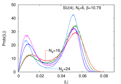
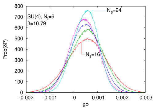
Figure 2: Histograms of $|L|$ and $\delta P$ normalized to have unit area under the curves. A multi-peak structure in the histogram corresponds to multiple (local) minima of the constrained free energy. As $N_{s}$ changes between the values shown, in steps of 2, the histograms move up or down monotonically in the region where they are labelled.

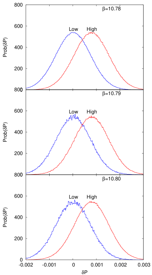
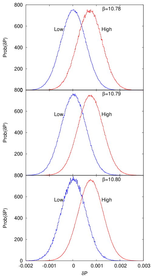
Figure 3: Histograms of $\delta P$ in the two phases of SU(4) gauge theory as defined using $L_{c}=0.024$ and $L_{h}=0.031$. The panels on the left are results from $6\times 16^{3}$ lattices and those on the right from $6\times 20^{3}$. The histograms are normalized so that the area under each is unity. The pure phase histograms at three different couplings exactly overlap on each lattice.

When two copies of a system with a first-order transition are held at temperatures $T_{c}\pm\delta T$, the difference in their energy densities is finite. Since the transition is of first-order, this difference remains finite even when $\delta T\to 0$, provided one has thermodynamically large systems. When $V$ is large but not infinite, the correct limit may be obtained as long as $\delta T/T_{c}$ is much larger than ${\cal O}(\xi^{3}/V)$. If $V$ is large enough, then this allows one to come close enough to $T_{c}$ to have confidence in the result. For smaller $\xi^{3}/V$, this procedure breaks down. By examining the reason for the breakdown, we can develop a different procedure to estimate the latent heat.

Finite-size effects at first-order phase transitions are best understood in terms of constrained free energies, $F_{c}$. This is the free energy of a system in which $|L|$ or $\delta P$ are restricted to have fixed values but other parameters are allowed to vary according to the temperature. $F_{c}$ near a first-order phase transition has multiple minima: the deepest corresponds to the value the constrained variable has in the stable phase when $V\to\infty$. As $T$ changes, the depth of the minima change, and on crossing $T_{c}$ the deepest minimum flips. However, because the finite system sees finite barriers between the minima, the system explores all the phases. Hence the discontinuity is rounded off. As the thermodynamic limit, $V\to\infty$, is approached, the “wrong phase” minimum becomes infinitely higher and the barrier separating it from the true vacuum also becomes infinitely high. As a result, the transition sharpens and gives the correct thermodynamic limit.

The histogram of an observable obtained from its Monte Carlo history is proportional to $\exp(-VF_{c}/T)$. The object of a finite-size scaling study of something like the latent heat is to be able to identify the thermodynamically stable phase from histograms such as those in Figure 2. The same figure also illustrates the problem which is usually faced in computing the latent heat in ${\rm SU}(N_{c})$ gauge theories. Although the histogram of $|L|$ has multiple well-identifiable maxima, the histogram of $\delta P$ has a single peak. If the specific heat in each of the phases is large, then the two-peak nature of $\Delta/T^{4}$ could well be hidden until extremely large volumes are reached. Finite-size scaling methods were developed in the past to extract reliably the specific heat when multiple maxima are clearly developed berg ; ohlsson . However they are not applicable here, and we need to use different techniques. We adapt one which was first applied to gauge theories in fukugita .

Since the phases are well resolved by $|L|$, we can try to use the following criterion. The cold confined phase could be identified by requiring that $|L|\leq L_{c}$, and the hot deconfined phase by $|L|\geq L_{h}$. The results of such a phase separation are stable as long as $L_{c}$ and $L_{h}$ both lie in the valley between the peaks of $|L|$. Examples of the probability density of $\delta P$ obtained in the cold and hot phases so defined are shown in Figure 3. The figures illustrate the fact that these probability densities are very stable— at each fixed volume the pure phase probability distributions of $\delta P$ are identical for a range of couplings around $T_{c}$. If we had not separated out the panels for different $\beta$, the curves for the three different cases would have been indistinguishable apart from small statistical fluctuations. Furthermore, as one changes $V$ (with fixed $a$) the mean value of $\delta P$ in the hot and cold phases remain the same. It appears that the difference between the values of $\delta P$ in the two phases is very stable under the variation of both $T$ and $V$ near $T_{c}$. It also turns out to be fairly stable under changes of $L_{c}$ and $L_{h}$.

The agreement of the histograms of $\delta P$ for the different $\beta$ in the transition regime show that it is possible to reliably extract the limiting values of $\Delta/T^{4}$ in each of the phases. Examination of (5) shows that knowing the difference in $\delta P$ between the hot and cold phases one can extract easily the jump in $\Delta/T^{4}$ and hence the latent heat density, since the remaining factors are well-understood. In Table 1 we summarize our results for the latent heat for ${\rm SU}(N_{c})$ gauge theories with $N_{c}=3$, 4 and 6. In the entry for the latent heat, the first error is statistical while the second is a systematic error, i.e., the change in the result if $L_{h}-L_{c}$ changes by $\pm$ 20%. The results of gavai are higher, but those of teper2 are consistent with ours, within the larger statistical and systematic errors of that study.

$N_{c}$	$N_{t}$	$N_{s}$	$\beta$	$|L|_{c}$	$|L|_{h}$	$\Delta\epsilon/T_{c}^{4}$	$\Delta\epsilon/\Delta_{\rm max\/}$
3	4	16	5.6908	0.055	0.075	2.06(1)(3)
		24	5.6919	0.055	0.075	1.93(1)(3)
		32	5.6922	0.055	0.075	1.90(2)(2)
	6	24	5.8934	0.02	0.03	1.79(2)(4)	0.65(2)
		32	5.8938	0.02	0.03	1.54(2)(5)
		48	5.8940	0.022	0.032	1.44(4)(3)
	8	32	6.0609	0.013	0.019	1.67(4)(4)	0.68(3)
4	6	16	10.79	0.024	0.031	4.85(5)(6)	0.88(2)
		20	10.79	0.024	0.031	4.64(4)(5)
		24	10.79	0.024	0.031	4.57(4)(3)	0.85(2)
	8	22	11.08	0.013	0.017	4.58(5)(6)
		24	11.08	0.013	0.017	4.32(6)(6)	0.82(2)
		28	11.08	0.013	0.017	4.33(8)(6))
	6	14	24.84	0.025	0.03	12.20(10)(4)
6		18	24.84	0.025	0.03	12.47(4)(2)	0.92(2)
	8	20	25.46	0.012	0.015	11.93(34)(5)	0.90(3)

Table 1: The latent heat of ${\rm SU}(N_{c})$ gauge theories for $N_{c}=3$, 4 and 6. The thermodynamic limit of $\Delta\epsilon/T_{c}^{4}$ is seen to be under control for $N_{c}=4$ and 6, as is the continuum limit. For all $N_{c}$, the ratio $\Delta\epsilon/\Delta_{\rm max\/}$ scales well. The numbers in brackets are the errors on the least significant digits, the first is statistical and the second systematic.

In SU(4) gauge theory we found that the extracted value of $\Delta\epsilon/T_{c}^{4}$ is fairly stable at fixed $a$ as we change $V$. In fact, as is clear from Table 1, when $a=1/(6T_{c})$ we found that there is no statistically significant change in the estimate of this quantity for $\zeta\geq 3$. The results for $a=1/(8T_{c})$ are consistent with this conclusion. For the SU(3) theory, on the other hand, it seems that $\zeta\geq 6$ is needed for an estimate of the latent heat with equally small systematic errors, i.e., finite volume corrections are larger for the SU(3) theory. One sees that in going from $N_{c}=3$ to 4 the latent heat density scales faster than $d_{A}$. This ties in with the intuition developed from a study of correlation lengths a1pp ; olaf that the SU(3) theory is weakly first-order. One expects that correlation lengths should also become shorter with increasing $N_{c}$ teper2 , and hence finite volume effects should be less pronounced.

Following the analysis of the appendix, we understand that the lack of clear scaling of $\Delta\epsilon/(d_{A}T^{4})$ to the continuum limit is not due to the use of an inappropriate beta-function. One possible explanation is that the large finite volume effects mask the approach to the continuum. If so, then one should be able to eliminate it by using another quantity with the same effect. Since $\Delta/T^{4}$ has a very sharp peak as a function of $T$, and that measurement would also be related to the latent heat, we list the quantity $\Delta\epsilon/\Delta_{\rm max\/}$ in the table. As one can see, this ratio has much better scaling properties, and the thermodynamic and continuum limits of the ratio are very well determined.

The data collected for $N_{t}=8$ in Table 1 is fitted extremely well by the form

$$\frac{\Delta\epsilon}{d_{A}T_{c}^{4}}=0.388(3)-\frac{1.61(4)}{N_{c}^{2}},$$ (9)

where the numbers in brackets are the statistical errors on the last digit of the central values. Interestingly, the fit yields $\Delta\epsilon/(d_{A}T_{c}^{4})=0.014\pm 0.014$ at $N_{c}=2$, where there is a second order finite temperature transition, and hence $\Delta\epsilon=0$. If one adds a term of ${\cal O}(1/N_{c}^{4})$, then the fit changes marginally: the limiting value for $N_{c}\to\infty$ is stable at the $3\sigma$ level. The coefficient of the ${\cal O}(1/N_{c}^{2})$ term changes by 16%, and the next correction term is marginal, its value being less than 10% of the total for $N_{c}=3$. The extended series extrapolated to $N_{c}=2$ is still consistent with vanishing latent heat of this theory. Although $N_{c}=2$ must be the limit of the validity of the series expansion around $1/N_{c}=0$, it seems to be well-behaved at $N_{c}=3$. In agreement with this, a reliable value of the $N_{c}\to\infty$ limit of $\Delta\epsilon/(d_{A}T^{4})$ can be extracted. This is an example of successful strong scaling; $\Delta\epsilon/(d_{A}T_{c}^{4})$ is well described by just two terms of the series in $1/N_{c}^{2}$ even at small $N_{c}$.

The series for the fourth root of the above quantity may be of interest, since $\sqrt[4]{\Delta}\epsilon$ has mass dimension unity teper1 ; teper2 . This gives

$$\left(\frac{\Delta\epsilon}{d_{A}T_{c}^{4}}\right)^{1/4}=0.798(7)-\frac{1.09(9)}{N_{c}^{2}}.$$ (10)

The quality of the fit, as judged by the value of $\chi^{2}/$DOF, is worse, but still within the limits of acceptability. This result above seems to have improved convergence properties around $N_{c}=\infty$. However, on extending the fit to include the ${\cal O}(1/N_{c}^{4})$ term, we find that the correction terms are unstable against changes. The coefficient of the second term reduces to half its value, and the coefficient of the third term is 6–7 times larger. The values of these terms are comparable to each other for $N_{c}=3$, opening the possibility that even higher order terms, or a resummation of the whole series, need to be taken into account. From the previous analysis it seems that the series expansion for $\Delta\epsilon/(d_{A}T_{c}^{4})$ comes close to performing this resummation. We shall show later that other mass dimension four quantities such as $p$, $\epsilon$ and $s$ also have good strong scaling properties.

IV Conformal symmetry breaking

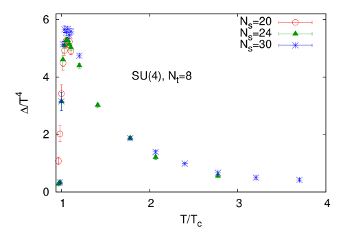
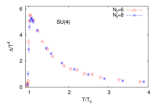
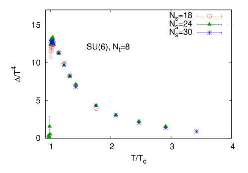
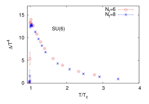
Figure 4: Systematics of $\Delta/T^{4}$ in SU(4) and SU(6) lattice gauge theories. Both finite size and finite lattice spacing effects are small, except, possibly, very close to $T_{c}$.

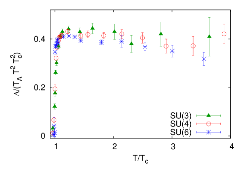
Figure 5: Testing a different scaling pisarski of the conformal symmetry breaking measure: $\Delta/(d_{A}T^{2}T_{c}^{2})$, where $d_{A}=N_{c}^{2}-1$, for $N_{c}=3$, 4, and 6.

As discussed in section II, $\Delta/T^{4}$ is easily calculated on the lattice. We have seen in the case of the latent heat, however, finite volume and cutoff effects need to be controlled. In the SU(3) gauge theory, it is known that $\Delta/T^{4}$ rises rapidly near $T_{c}$ and peaks at about $1.1T_{c}$ boyd . The rapid rise is, of course, dictated by the existence of a latent heat, but the shift in the peak away from $T_{c}$ is not yet understood. We examine the $N_{c}$ dependence of this peak.

In Figure 4, we show the sensitivity of $\Delta/T^{4}$ to $\zeta$ and $a$. Except in the immediate vicinity of $T_{c}$ there seems to be little sensitivity to $\zeta$. The cutoff dependence is also insignificant, except in the vicinity of the peak, $\Delta_{\rm max\/}$. The good agreement between data obtained with $a=1/(6T)$ and $1/(8T)$ show that the results of the measurement with either lattice spacing can be taken to be an estimate of the continuum limit. We choose the conservative alternative of using $a=1/(8T)$ as a determination of the continuum results. The peak of $\Delta/T^{4}$ for SU(4) gauge theory is in the range $1.04\leq T/T_{c}\leq 1.08$.

The systematics of $\Delta/T^{4}$ for SU(6) gauge theories is also shown in the same figure. The trends are very similar to those in SU(4). Results for different $\zeta$ agree very well. The approach to the continuum limit is also very similar to that discussed for SU(4). Again, in this case, we can take the results obtained with $a=1/(8T)$ to be an estimate of the continuum limit. In going from $N_{c}=3$ to 6, the peak in $\Delta/T^{4}$ moves closer to $T_{c}$.

It is of phenomenological interest to note that $\Delta/T^{4}$ is not small even at $2T_{c}$. In fact, as one can see in Figure 4, one has

$$\left.\frac{\Delta}{T^{4}}\right|_{2T_{c}}\simeq 0.1d_{A}.$$ (11)

For $N_{c}=3$ this implies $\Delta^{1/4}\simeq T=2T_{c}$. This is a natural scale, and therefore the theory is far from conformal.

We end this section with the investigation of an intriguing observation made in ogilvie ; pisarski : in the temperature range $1.1T_{c}\leq T\leq 4T_{c}$, for the SU(3) pure glue plasma, $\Delta/T^{2}$ seems to be roughly constant. Phenomenological models of the gluon plasma have introduced mass scales and obtained such a behaviour pheno . We investigated this modified scaling behaviour at larger $N_{c}$ (see Figure 5). The dimensionless quantity $\Delta/(d_{A}T^{2}T_{c}^{2})$ for SU(3) gauge theory is seen to have little temperature dependence from just above $T_{c}$ to about $4T_{c}$. Unfortunately, the data for SU(3) theory is noisy at larger $T$. For SU(6) the error bars are smaller and one can observe that this quantity falls with $T$. This implies that the temperature dependence of $\Delta$ could be slower than $T^{2}$. It would be interesting in future to expand the range of $N_{c}$ and $T$ in order to study this further.

V Other bulk thermodynamic quantities

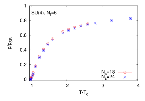
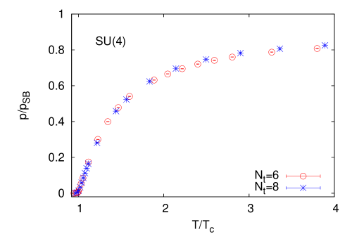
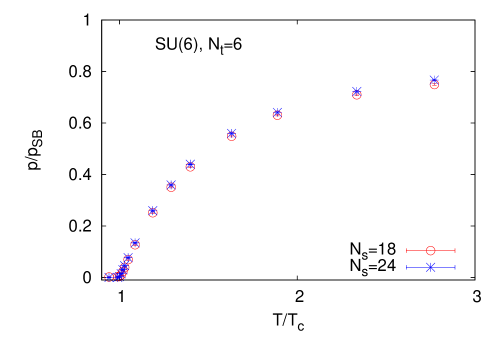
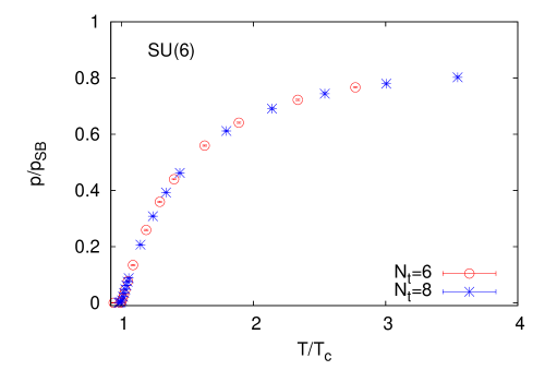
Figure 6: Study of systematics in the calculation of pressure for SU(4) and SU(6) gauge theory. Both finite size and finite lattice spacing effects seem to be under control.

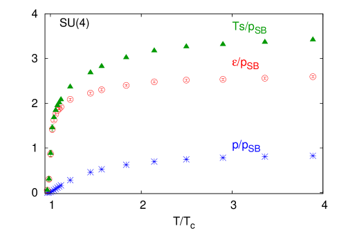
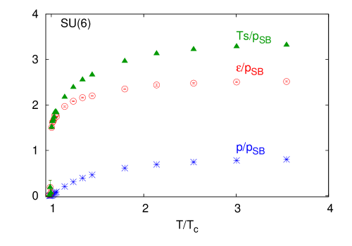
Figure 7: Results for thermodynamic quantities in SU(4) (left) and SU(6) (right) gauge theories. Shown are the pressure, energy density and entropy density, in units of $p_{\scriptscriptstyle SB}$. The ideal gas limits for these quantities should be 1, 3 and 4 respectively.

The pressure is calculated using the method outlined in (6). The integration requires interpolation of the measured points, and there could be a systematic error arising from this. We have estimated this error by comparing linear and quadratic interpolations. We found that point by point the error is small. Since the integration errors increase over the range of $\beta$ and reach a maximum at the highest $\beta$ that we use, it is sufficient to report the magnitude of that error compared to the statistical uncertainty. We can estimate the significance of the error by the $t$-statistic—

$$t=\frac{\left|I_{2}-I_{1}\right|}{\sqrt{\sigma^{2}(I_{2})+\sigma^{2}(I_{1})}}$$ (12)

where $I_{2}$ is the integral estimates through a quadratic interpolation, $I_{1}$ is the estimate using a linear interpolation and $\sigma^{2}(I_{1,2})$ is the statistical error in the estimate of $I_{1,2}$. This measure for SU(4) is 1.03 and for SU(6) it is 0.007. This source of error is therefore almost negligible. As a result, the systematic error is almost entirely due to the neglect of $p_{0}$, the pressure at the lowest temperature where the integration is started.

Figure 6 shows the cutoff and volume dependence in the calculation of pressure for the SU(4) and SU(6) theories. The results are normalized by the known (asymptotic) finite cutoff correction for an ideal gluon gas, $p_{\scriptscriptstyle SB}$, which was described earlier. Hence the pressure, so normalized, should go to unity. We find that finite volume effects are negligible. Finite lattice spacing effects also turn out to be negligible once we normalize the pressure by $p_{\scriptscriptstyle SB}$ . These results indicate that it is safe to identify the continuum limit with the $N_{t}=8$ measurements. Since the volume dependence is negligible, at each $T$ we use the largest volume on which reliable results are available as an indication of the thermodynamic limit.

At asymptotically large $T$ the ${\rm SU}(N_{c})$ gauge theory should go over to the ideal gluon gas. However, even at the highest temperatures which we have probed, i.e., $T\simeq 4T_{c}$, the ratio $p/p_{\scriptscriptstyle SB}$ is far from unity (see Figure 6). Given $p/T^{4}$ and $\Delta/T^{4}$ we obtain also the other bulk thermodynamic quantities: $\epsilon/T^{4}$ and $s/T^{3}$. These results are collected in Figure 7. One sees clear deviations from the ideal gas limit in these two quantities as well. All three quantities also show a very slow rise throughout the measured range of $T$. Both $\epsilon$ and $s$ show a rapid jump near $T_{c}$, stronger for SU(6) than for SU(4).

VI $N_{c}$ scaling of thermodynamic observables

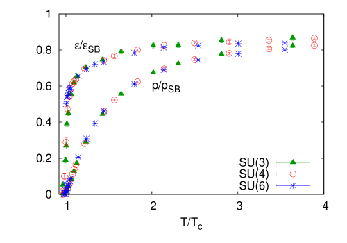
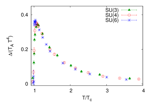
Figure 8: The first panel shows the energy density and pressure in ${\rm SU}(N_{c})$ pure gauge theories, normalized to the corresponding ideal gas values. The second panel shows $\Delta/T^{4}$, normalized by $d_{A}=N_{c}^{2}-1$, for the same theories.

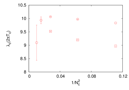
Figure 9: The value of the ’t Hooft coupling at the finite temperature transition, $\lambda_{c}$, for different $N_{c}$. The renormalized gauge coupling is evaluated at scale of $2\pi T_{c}$, so that the result is independent of the lattice spacing. The boxes denote results obtained using the non-perturbative beta-function and the circles using the two-loop beta-function in the V-scheme.

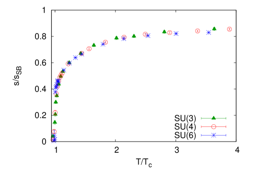
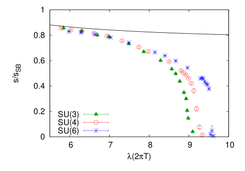
Figure 10: The scaled entropy density, $s/s_{\scriptscriptstyle SB}$, as a function of $T/T_{c}$ and the ‘t Hooft coupling $\lambda=N_{c}g_{R}^{2}$. The gauge coupling is evaluated at the scale $2\pi T$ using the non-perturbative beta-function for the appropriate theory.

As discussed earlier, we distinguish between strong $N_{c}$ scaling and ’t Hooft scaling. The first is scaling with $N_{c}$ of thermodynamic quantities at fixed $T/T_{c}$, and the second, the scaling with $N_{c}$ at fixed $\lambda$. We examine scaling by combining our results for the continuum limit of bulk thermodynamic quantities for $N_{c}=4$ and 6, with a reanalysis of the older $N_{c}=3$ data of boyd using our techniques.

Strong $N_{c}$ scaling has been observed on the lattice in many contexts teper1 ; teper2 ; barak ; panero . The continuum limit of bulk thermodynamic quantities that we have extracted are also consistent with this limiting procedure, except for $N_{c}=3$ near $T_{c}$. In Figure 8 we show the energy density and pressure, each normalized by its ideal gas value, for $N_{c}=3$, 4 and 6. As noted earlier, there are clear deviations from the ideal gas behaviour, but the scaled quantities are almost independent of $N_{c}$. Since the ideal gas values scale with $d_{A}$, one expects that at large $T$ all bulk thermodynamic quantities should scale accordingly.

We see that $p/p_{\scriptscriptstyle SB}$ is independent of $N_{c}$ over the whole temperature range above $T_{c}$ within the accuracy of our measurement. Such a statement is also true for the energy density except when $T$ is close to $T_{c}$. Close to $T_{c}$ the energy density does not scale as the ideal gas, i.e., as $d_{A}$, between $N_{c}=3$ and larger values of $N_{c}$. This is, of course, a consequence of the fact that the latent heat density does not scale as $d_{A}$ for $N_{c}=3$ (see Table 1). Consequently, $\Delta/T^{4}$ also fails to scale with $d_{A}$ in the vicinity of $T_{c}$. In Figure 8 we also show that the peak of $\Delta/(T^{4}d_{A})$ is smaller for $N_{c}=3$ than for $N_{c}=4$ and 6 (the latter two are almost identical in value). We also see that the peak is rounded and shifted away from $T_{c}$ at $N_{c}=3$. As discussed in Section III, this could be due to finite-size effects, since $N_{c}=3$ has a weaker first-order phase transition. With this exception, strong $N_{c}$ scaling seems to work very well for bulk thermodynamic quantities; the sub-leading corrections are too small to be seen over the statistical errors.

Next we turn to evidence for ’t Hooft scaling. Since the critical point is known very precisely for several $N_{c}$ scaling , we test this scaling using $\lambda_{c}=N_{c}g_{R}^{2}(2\pi T_{c})$ . The change of $\lambda_{c}$ with $N_{c}$ is very much larger than the statistical errors, and is seen using both the non-perturbative and the two-loop beta-functions, although it is somewhat larger with the former. The change is non-monotonic when the two-loop beta-function is used. In this context, we recall the result shown in the appendix: that the non-perturbative beta-function is preferred near $T_{c}$. Restricting ourselves to using only this leaves the three smallest values of $N_{c}$.

Even with these three, it is clear from Figure 9 that the data do not fall on a straight line and hence a single correction term does not suffice. Using a second correction term, a description of the confinement-deconfinement phase boundary, i.e., the variation of $\lambda_{c}$ with $1/N_{c}^{2}$, is—

$$\lambda_{c}=\begin{cases}9.8771(4)-\frac{14.2562(2)}{N_{c}^{2}}+\frac{54.7830(2)}{N_{c}^{4}}&\text{(non-perturbative),}\\ 9.9904(6)+\frac{1.2081(3)}{N_{c}^{2}}-\frac{23.5709(3)}{N_{c}^{4}}&\text{(two-loop).}\end{cases}$$ (13)

Since the fit is linear in the parameters, the formal solution for $\chi^{2}$ minimization can be written down along with parameter errors. At $N_{c}=3$ the values of the ${\cal O}(1/N_{c}^{2})$ and ${\cal O}(1/N_{c}^{4})$ terms are comparable. Although they are small corrections to the leading, ${\cal O}(N_{c}^{0})$ term, this behaviour of the series could indicate that $N_{c}=3$ lies near the radius of convergence of the series around $N_{c}=\infty$.

If this is so, then summing three terms of the series is not numerically accurate. However, with three pieces of data fitting a large number of terms is an ill-conditioned problem. As a result, one would do better to fit a resummation of the series, provided such a resummation has a small number of parameters. Unfortunately, there is no theory for the shape of the phase boundary. In its absence we try the usual trick of estimating a Padé resummation of the series. With three terms the best that we can try to do is to fit the lowest order expansion

$$\lambda_{c}(N_{c})=\lambda_{c}(\infty)+\frac{a/N_{c}^{2}}{1+N_{*}^{2}/N_{c}^{2}}.$$ (14)

The best fit gives $N_{*}\simeq 4$, roughly consistent with the series analysis. As a result, the fitted value of $\lambda_{c}(\infty)$ is sensitive to the form of the remaining function, and cannot be reliably extracted using data for $N_{c}$ near 4. It would be useful to improve the computations with $N_{c}>6$ in order to extract this quantity with better accuracy.

Next, we extend such a test to a bulk thermodynamic quantity. Our results for $s/s_{\scriptscriptstyle SB}$ as functions of $T/T_{c}$ and $\lambda(2\pi T)$ are shown in Figure 10. As we show in the figure, strong scaling holds with good precision since $s/s_{\scriptscriptstyle SB}$ is almost independent of $N_{c}$ down to the smallest temperatures that we have studied. For scaling at fixed $\lambda$, convergence of the series is clearly bad for $\lambda\simeq 9$ or larger, because the theories for different $N_{c}$ begin to drop out of the plasma phase; figure 9 shows that theories with smaller $N_{c}$ drop to the confined phase at smaller $\lambda$. At any fixed $\lambda$ in this region one has to go to $N_{c}$ large enough that the theories are all in the same phase before one can observe good scaling with $N_{c}$. We also find that the convergence of the series in $1/N_{c}^{2}$ is acceptable when $\lambda<8.6$ . In the range $8.6<\lambda<9$, the physically interesting theory with $N_{c}=3$ is close to the radius of convergence of the series expansion, and the effect of the correction terms is large.

Figure 10 also displays a comparison of the scaled entropy with predictions in a ${\cal N}=4$ supersymmetric Yang-Mills theory, computed gubser using the AdS/CFT correspondence—

$$\frac{s}{s_{\scriptscriptstyle SB}}=\frac{3}{4}+\frac{45}{32}\zeta(3)\left(\frac{1}{\lambda}\right)^{3/2}+\cdots.$$ (15)

Although one does not expect this computation to be valid in the realistic non-supersymmetric theories under investigation, it is sometimes said to agree with lattice results. Here we show that the agreement is poor, except at the highest possible temperatures. It has been argued panero that more realistic AdS-QCD models should be used for such a comparison; the analysis of such models lies beyond the scope of this paper.

VII Summary and Discussion

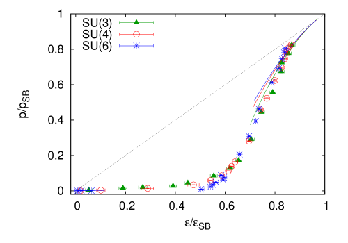
Figure 11: Approach to conformality in ${\rm SU}(N_{c})$ gauge theories. The diagonal line contains results from all possible conformal theories; the upper right end is the special case of a free massless theory. Also shown are the weak coupling results from mikko (with increasing $N_{c}$ the curves move up monotonically). Since the lattice data lie closer to the weak-coupling results than to the diagonal line, there seems to be no window where a strongly coupled conformal theory describes ${\rm SU}(N_{c})$ pure gauge thermodynamics.

In this paper we have studied the thermodynamics of the gluo$N_{c}$ plasma, by numerical simulations of SU(4) and SU(6) gauge theories, and comparing them with a reanalysis of existing data boyd for SU(3). Our focus is on taking the continuum and thermodynamic limits, by using multiple spatial volumes at each cutoff and by using significantly smaller cutoffs than used previously for the EOS of $N_{c}>3$. As discussed in the introduction, in terms of statistics, lattice spacing and spatial volumes, this work brings the study of the thermodynamics of pure gauge ${\rm SU}(N_{c})$ theories with small $N_{c}>3$ at par with the state of the art for $N_{c}=3$, while also throwing some new light on the SU(3) theory.

We had shown in an earlier study of the deconfinement transition scaling that observations made with finite lattice spacing could be continued to the continuum using the renormalization group equations. When measurements are made with lattice spacing $a\leq 1/(8T_{c})$ we had found that the two-loop beta-function suffices. When the lattice spacing $a=1/(6T_{c})$ is used a non-perturbative beta-function was introduced which could be used to continue the lattice results to the continuum limit scaling . In this paper we used these earlier results to obtain the continuum thermodynamics of pure gauge SU(4) and SU(6) theories. We also made a reanalysis of the older SU(3) data using this technique (as detailed in the appendix).

One of our important results (see Section III) is an extraction of the latent heat of the deconfinement transition, $\Delta\epsilon/T_{c}^{4}$, for $N_{c}=3$, 4 and 6. We found that $\Delta\epsilon/(d_{A}T_{c}^{4})$, where $d_{A}=N_{c}^{2}-1$, increases between $N_{c}=3$ and larger $N_{c}$, indicating that the first-order transition grows stronger with increasing $N_{c}$. Our results are compatible with teper2 . One expects stronger transitions to have smaller finite volume effects, and our observations support this notion. We found some scale breaking in the measurement of $\Delta\epsilon/T_{c}^{4}$, and observed that $\Delta\epsilon/\Delta_{\rm max\/}$ shows better scaling properties. We also saw that in the large $N_{c}$ limit one has $\Delta\epsilon/(d_{A}T_{c}^{4})=0.388\pm 0.003$ (see eq. 9).

Further study of bulk thermodynamic quantities started with measurements of $\Delta/T^{4}$ (details are given in Section IV). We found good scaling of this quantity, and a reliable continuum limit, for $T>T_{c}$. For SU(3) some scale breaking is observed very close to $T_{c}$ where the peak of this quantity lies. The cause remains obscure, although there are some indications that lead us to conjecture that this could be due to finite volume effects. Future studies are planned to understand this remaining ambiguity. In a range of temperature up to $4T_{c}$ we found that $\Delta\propto T^{2}$ ogilvie ; pisarski , or, possibly, slower.

The pressure, $p/T^{4}$, was obtained using the so-called integral method (see Section V). Finite volume and lattice spacing effects in this measurement are under good control. We extracted the energy density, $\epsilon/T^{4}$, and the entropy density, $s/T^{3}$, using these two primary measurements. In the whole range of $T$ all these quantities lie substantially below the ideal gas values (see Figures 7 and 8). Nevertheless, $p/T^{4}$, considered as a function of $T/T_{c}$, scales very well with $d_{A}$ barak ; panero . Sub-leading corrections in $N_{c}$ are hard to see at the level of accuracy we have reached (see Figure 8). Similar scaling with $d_{A}$ is also seen for $\epsilon/T^{4}$ and $s/T^{4}$, except, possibly, in a small region near $T_{c}$.

In Figure 11 we present a plot of the normalized energy density, $\epsilon/\epsilon_{\scriptscriptstyle SB}$ against the normalized pressure, $p/p_{\scriptscriptstyle SB}$ following swagato . The diagonal line is the line of all conformal theories, with the ideal gluon gas being one special point on it. Weak coupling results mikko lie below this. One sees that the lattice data for $N_{c}=3$, 4 and 6 lie further below. Indeed the topology of these relations is such that the weak coupling predictions are always a better approximation to the lattice data than conformal theories. This figure gives clear evidence that there is no window of temperature in which the EOS can be described by a strongly-coupled conformal theory better than by weak coupling theory.

Yet another reason for making high-precision measurements of bulk thermodynamics for $N_{c}\neq 3$ is to understand the usefulness of the large-$N_{c}$ limit (see Section VI). In agreement with previous results, we find that the strong scaling limit obtained by taking fixed $T$ and $N_{c}\to\infty$ works very well. Corrections in powers of $1/N_{c}$ are small, as a result of which the large-$N_{c}$ results for the entropy density, for example, can be directly applied for $N_{c}=3$ with about 1% error. However, when the same data is analyzed as a function of the ’t Hooft coupling, the finite $N_{c}$ corrections are large for $\lambda>8.6$. The phase boundary for the large $N_{c}$ theory, expanded in powers of $1/N_{c}^{2}$, seems to have a radius of convergence smaller than 1/9 (see eq. 14). Since this observation has ramifications for all models of thermal QCD which proceed from the large-$N_{c}$ approximation, including string-based models, we plan further measurements in the near future to explore the applicability of the ’t Hooft limit.

We thank Mikko Laine for providing us with the weak coupling results of Fig. 11 and Rob Pisarski for comments. The computations were carried out on the workstation farm of the department of theoretical physics, TIFR and the Cray X1 of the ILGTI. We thank Ajay Salve for technical support.

Appendix A The beta-function

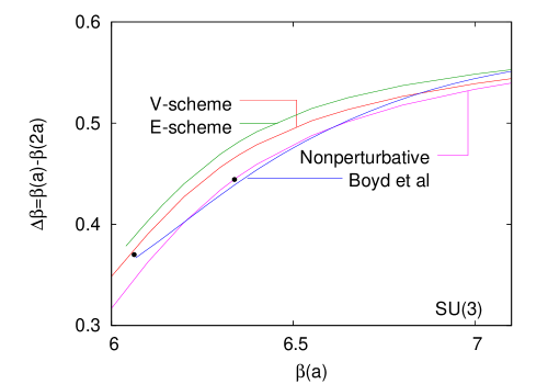
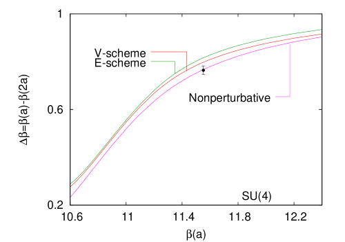
Figure 12: The step scaling function in SU(3) (left) and SU(4) (right) gauge theory. The data points are for the location of the deconfinement transition. For SU(3) they are taken from boyd ; fingberg and for SU(4) from scaling . The non-perturbative beta-function of boyd is tuned for use with $a\leq a_{c}(4)$. We have used a non-perturbative beta-function precise ; scaling which can be used for $a<a_{c}(6)$.

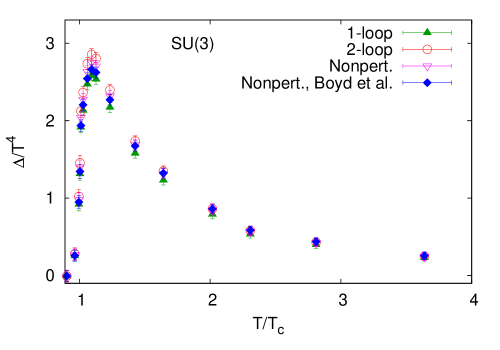
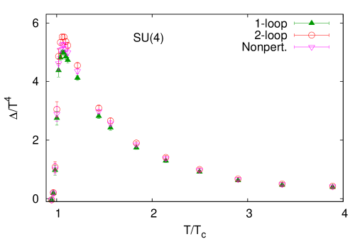
Figure 13: $\Delta/T^{4}$ for SU(3) gauge theory on $32^{3}\times 8$ lattices (left) and SU(4) on $30^{3}\times 8$ lattices (right). Shown are the analyses using various different beta-functions (based on the V-scheme). For SU(3), where the data is taken from boyd we also show the analysis using the non-perturbative beta-function of that paper.

The lattice theory is cut off at a length scale of $a$. When $a$ is small various quantities have a perturbation expansion in $g_{R}$, the renormalized coupling determined at a scale $\kappa a$ (where $\kappa$ can depend on the scheme). Then the derivative in eq. (5) can be written as

$$\frac{\partial\beta}{\partial\ln a}=\frac{\partial\beta}{\partial g_{R}}\frac{\partial g_{R}}{\partial\ln a},$$ (16)

where the last factor is the negative of the beta-function. Due to the fact that ${\rm SU}(N_{c})$ gauge theories are asymptotically free, one expects that a weak-coupling determination of the beta-function should suffice when $a$ is small enough. In scaling it was shown that the two-loop beta-function is a sufficient description of the flow of the renormalized coupling at the scale of $a\leq 1/(8T_{c})$. Confidence in the efficacy of two-loop scaling is enhanced by the fact that the scheme dependence in the extraction of the QCD scale was small.

Although the two-loop beta-function was insufficient to describe the flow of the coupling at larger $a$, it was shown that for $a\simeq a_{c}(6)$, where $a_{c}(N_{t})=1/(N_{t}T_{c})$, a simple correction of the form

$$a_{c}(N_{t})\Lambda=R\left(\frac{1}{\beta_{0}g_{R}^{2}(a_{c})}\right)\,\left[1+\frac{c_{2}}{N_{t}^{2}}\right],\qquad{\rm with}\qquad R(x)={\rm e}^{-x/2}x^{\beta_{1}/2\beta_{0}^{2}}$$ (17)

suffices, where the two-loop beta-function is $-\beta_{0}g_{R}^{3}-\beta_{1}g_{R}^{5}$ (for an alternative approach see alphas ). The values of $c_{2}$ were presented in Table (iv ) of scaling . In this paper the integration of the beta-function is started from the scale $a_{c}(8)$. In the calculation of section IV, since we have taken data at lattice spacings as low as $a_{c}(6)$, we have used such a non-perturbatively corrected beta-function in the V-scheme (this differs from the conventions of qm09 ). Any non-perturbative beta-function will include finite lattice spacing corrections allton into the scaling, just as the above function does. Such corrections are non universal.

A simplified version of the tests of scaling in precise ; scaling can be presented using the step-scaling function $\Delta\beta(\beta)$. This is the change in the bare coupling, $\Delta\beta$, required to reproduce the physics observed at a bare coupling $\beta$, when the lattice spacing is doubled. If $\beta$ is chosen to be the lattice coupling where the deconfinement transition is observed for a given $N_{t}$, then $\beta-\Delta\beta$ is the lattice coupling at the deconfinement transition when $N_{t}$ is changed to $N_{t}/2$. In Figure 12 we show the result of using the beta-functions given above and the step scaling function given in boyd .

We also examined the sensitivity of the equation of state to the choice of the beta-function. Figure 13 displays results for $\Delta/T^{4}$ obtained in SU(3) and SU(4) gauge theory, for lattices with $a=1/(8T)$. For the SU(4) theory, differences between the E-scheme and the V-scheme are statistically insignificant at all temperatures. Similarly, the difference between these and the non-perturbative beta-function of (17) are also insignificant at these temperatures.

The results are similar for the SU(3) gauge theory, where we have re-analyzed the data of boyd . The one-loop and the two-loop beta-functions give coincident results for $T\geq 1.5T_{c}$. In precise a non-perturbative beta-function of the form in (17)) was used to describe scaling of $T_{c}$. The results of using this for $\Delta/T^{4}$ are shown. These three are close to each other, as is the result of boyd .

References

- (1) G. ’t Hooft, Nucl. Phys., B 72 (1974) 461.
-
(2)
See, for example,
E. Brezin, C. Itzykson, G. Parisi and J.-B. Zuber,
Comm. Math. Phys., 59 (1978) 35;
E. Witten, Nucl. Phys., B 156 (1979) 269;
T. Eguchi and H. Kawai, Phys. Rev. Lett., 48 (1982) 1063;
S. Coleman, in Aspects of Symmetry, Cambridge University Press, 1985, Cambridge, UK;
E. Brezin and S. Wadia, The large N expansion in quantum field theory and statistical physics, World Scientific, 1993, Singapore;
M. J. Teper, Phys. Rev., D 59 (1998) 014512. - (3) S. Datta and S. Gupta, Nucl. Phys., A 830 (2009) 749C, PoS(LAT2009) 178.
- (4) R. Pisarski and L. McLerran, Nucl. Phys., A 796 (2007) 83.
- (5) M. Wingate and S. Ohta, Phys. Rev., D 63 (2001) 094502;
- (6) R. V. Gavai, Nucl. Phys., B 633 (2002) 127.
- (7) B. Lucini, M. Teper and U. Wenger, Phys. Lett., B 545 (2002) 197, J. H. E. P., 0401 (2004) 061;
- (8) B. Lucini and M. Teper, J. H. E. P., 0502 (2005) 033.
- (9) S. Datta and S. Gupta, Phys. Rev., D 80 (2009) 114504.
- (10) B. Bringoltz and M. Teper, Phys. Lett., B 628 (2005) 113.
- (11) M. Panero, Phys. Rev. Lett., 103 (2009) 232001, PoS(LAT2009) 172.
- (12) See EPAPS Document no. [epaps doc] for a listing of the run parameters, statistics and autocorrelation times.
- (13) G. Boyd et al., Nucl. Phys., B 469 (1996) 419.
- (14) J. Engels, F. Karsch and T. Scheideler, Nucl. Phys., B 564 (2000) 303.
- (15) S. Datta and S. Gupta, Phys. Rev., D 67 (2003) 054503.
- (16) O. Kaczmarek et al., Phys. Rev., D 62 (2000) 034021.
- (17) N. A. Alves, B. A. Berg and R. Villanova, Phys. Rev., B 43 (1991) 5846.
- (18) S. Gupta, A. Irbäck and M. Ohlsson, Nucl. Phys., B 409 (1993) 663.
- (19) M. Fukugita, M. Okawa and A. Ukawa, Phys. Rev. Lett., 63 (1989) 1768.
- (20) P. N. Meisinger, T. R. Miller and M. C. Ogilvie, Phys. Rev., D 65 (2002) 034009.
- (21) R. Pisarski, Prog. Theor. Phys. Suppl., 168 (2007) 276.
-
(22)
E. Megias, E. Ruiz Arriola and L. L. Salcedo, Phys. Rev., D 80 (2009) 056005;
V. Gogokhia, M. Vasuth and V. V. Skokov, J. Phys., G 37 (2010) 075015. - (23) M. Laine and Y. Schroder, J. H. E. P., 0503 (2005) 067.
-
(24)
S. S. Gubser, I. R. Klebanov and A. A. Tseytlin,
Nucl. Phys., B 534 (1998) 202;
I. R. Klebanov, eprint hep-th/0009139, Lecures given at TASI 99; J.-P. Blaizot, E. Iancu, U. Kraemmer and A. Rebhan, J. H. E. P., 0706 (2007) 035. - (25) R. V. Gavai, S. Gupta and S. Mukherjee, Phys. Rev., D 71 (2005) 074013.
- (26) M. Laine and Y. Schroder, Phys. Rev., D 73 (2006) 085009.
- (27) J. Fingberg et al., Nucl. Phys., B 469 (1996) 419.
- (28) S. Gupta, Phys. Rev., D 64 (2001) 034507.
-
(29)
C. Allton, M. Teper and A. Trivini, J. H. E. P., 0807 (2008) 021;
B. Lucini and G. Moraitis, Phys. Lett., B 668 (2008) 226. - (30) C. R. Allton, hep-lat/9610016.