The physical and dynamical structure of Serpens

Abstract

Context. The Serpens North Cluster is a nearby low mass star forming region which is part of the Gould Belt. It contains a range of young stars thought to correspond to two different bursts of star formation and provides the opportunity to study different stages of cluster formation.

Aims. This work aims to study the molecular gas in the Serpens North Cluster to probe the origin of the most recent burst of star formation in Serpens.

Methods. Transitions of the C¹⁷O and C¹⁸O observed with the IRAM 30m telescope and JCMT are used to study the mass and velocity structure of the region while the physical properties of the gas are derived using LTE and non-LTE analyses of the three lowest transitions of C¹⁸O.

Results. The molecular emission traces the two centres of star formation which are seen in submillimetre dust continuum emission. In the $\sim$40 M_⊙ NW sub-cluster the gas and dust emission trace the same structures although there is evidence of some depletion of the gas phase C¹⁸O. The gas has a very uniform temperature ($\sim$10 K) and velocity ($\sim$8.5 kms^-1) throughout the region. This is in marked contrast to the SE sub-cluster. In this region the dust and the gas trace different features, with the temperature peaking between the submillimetre continuum sources, reaching up to $\sim$14 K. The gas in this region has double peaked line profiles which reveal the presence of a second cloud in the line of sight. The submillimetre dust continuum sources predominantly appear located in the interface region between the two clouds.

Conclusions. Even though they are at a similar stage of evolution, the two Serpens sub-clusters have very different characteristics. We propose that these differences are linked to the initial trigger of the collapse in the regions and suggest that a cloud-cloud collision could explain the observed properties.

1 Introduction

Despite the importance of understanding the processes driving the formation of stars in the Galaxy, little is known about the role played by molecular cloud kinematics on triggering or suppressing star formation. Since most stars form in clusters (Lada & Lada, 2003), the kinematics of young stellar clusters in which the initial conditions of clustered star formation are still imprinted in the gas and dust emission properties can provide important insights into the dominant mode of star formation (e.g. Peretto et al., 2006).

Table 1: Submillimetre sources in Serpens Main Cluster

Source name	RA (J2000)	Dec (J2000)	offset RA (′′)	offset Dec (′′)
SMM 1	18:29:49.87	1:15:16.0	0.3	2.6
SMM 2	18:30:00.25	1:12:51.7	0.8	5.7
SMM 3	18:29:59.26	1:13:56.3	0.3	2.0
SMM 4	18:29:56.77	1:13:08.0	2.7	2.1
SMM 5	18:29:51.35	1:16:34.9	3.3	0.9
SMM 6	18:29:57.99	1:13:59.2	4.7	3.0
SMM 8	18:30:01.88	1:15:08.4	0.5	0.9
SMM 9	18:29:48.34	1:16:42.0	3.3	0.5
SMM 10	18:29:52.04	1:15:44.4	1.5	3.4
SMM 11	18:30:00.41	1:11:41.6	1.4	0.8

One such young and nearby cluster is in the Serpens Molecular Cloud (MC). Located at $\sim$260 pc (Straižys et al., 1996), the optical extinction map of the cloud covers more than 10 deg² (Cambrésy, 1999). However, the majority of the star formation is occuring in three clusters covering approximately 1.5 deg² (Enoch et al., 2007). The most active region is the Serpens Main Cluster (hereafter Serpens) which has a surface density of YSOs of 222 pc^-2, compared to 10.1 pc^-2 in the rest of the Serpens cloud (Harvey et al., 2007a). In this main cluster, the average gas density is around 10⁴ cm^-3 (Enoch et al., 2007) with H₂ column densities greater than 10²² cm^-2 in the cores. The high density of protostars in this main cluster seems to indicate an early stage of evolution where the cluster gas may still be infalling into the cores (Williams & Myers 1999; 2000;Hurt et al. 1996). The star formation rate in this main cluster is 56 M_⊙Myr^-1pc^-2, $\sim 20$ times higher than in the rest of the cloud (Harvey et al., 2007a).

Amongst the youngest YSOs found in Serpens there are ten Class 0 and I protostars which are detected in 850 $\mu$m dust continuum emission (e.g. Hurt & Barsony 1996, Davis et al. 1999), hereafter referred to as submillimetre sources (shown on Fig. 1, Table 1 and discussed on Sec. 2.2). These are distributed within $\sim$ 0.2 pc² and divided between two sub-clusters, one to the northwest (NW) and one to the southeast (SE). These submillimetre sources power a number of outflows, which have been studied using several different approaches (e.g. Eiroa et al., 1992; Davis et al., 1999; Hodapp, 1999; Davis et al., 2000; Graves et al., 2010). Figure 1 also shows the Spitzer MIPS 24 $\mu$m emission tracing the young protostars classified as Class I or 0. The oldest objects in the area shown on the image are a few flat spectrum sources (Harvey et al., 2007a; Kaas et al., 2004). The presence of Class II and Class III objects (not shown in Figure 1) dispersed over a larger area suggests that the region has undergone two episodes of star formation. The first, responsible for these dispersed pre-main sequence stars (the Class II and III sources), occurred about 2 Myr before the most recent burst which formed the submillimetre and 24$\mu$m protostars (Class 0, I and flat spectrum sources), $\leavevmode\nobreak\ 10^{5}$ yr ago (Harvey et al., 2007a; Kaas et al., 2004).

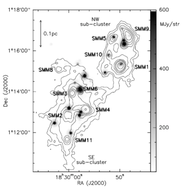
Figure 1: Map of the SCUBA 850 $\mu$m continuum emission in contours showing the position of the submillimetre sources (labeled). Contours at 0.4, 0.6, 1, 1.4, 1.8, 2.4 and 5 Jy beam^-1. In grey scale are the Spitzer MIPS 24 $\mu$m sources (Harvey et al., 2007b). All the sources seen on this figure are classified as being young protostars, mostly Class O and Class I sources, with a small number of flat spectrum sources.

This paper focuses on the dynamical and physical properties of the gas in Serpens using CO isotopologues observed with the IRAM 30m telescope and with JCMT, to probe the current properties of the region as well as investigate any link back to the initial conditions under which the most recent burst of star formation in Serpens took place. Section 2 presents the observations, as well as the data reduction and analysis methods and techniques used in this study. In Section 3 the structure of the gas is discussed while Section 4 discusses its dynamics. In Section 5 its physical properties are analysed. These results are drawn together and a scenario for the origin of the star formation in Serpens described in Section 6.

2 Data and Analysis Techniques

2.1 IRAM Observations

The Serpens region was observed in the J=1$\rightarrow$0 and J=2$\rightarrow$1 transitions of C¹⁸O and the J=1$\rightarrow$0 transition of C¹⁷O with the IRAM 30m telescope, using the facility receivers, in May 2001. The observations consisted of on-the-fly maps of the region, centered at RA = $18^{h}$$29^{m}$$57.91^{s}$ and Dec = $1^{\circ}$$12^{\prime}$$25.2^{\prime\prime}$ over an area of approximately 10.5 arcmin², $\sim$ $3^{\prime}$ in Right Ascension and $3.5^{\prime}$ in Declination.

The C¹⁷O J=1$\rightarrow$0 data, observed at 112.359 GHz, have a spatial resolution of $22^{\prime\prime}$, a velocity resolution of $\sim$ 0.052 kms^-1 and a noise level of $\sim$ 0.45 K (in T${}_{\mathrm{A}}^{*}$) in the raw map – low enough to allow the detection and identification of the hyperfine components of the J=1$\rightarrow$0 transition of C¹⁷O. C¹⁸O was observed with spectral resolution of $\sim$ 0.053 kms^-1 at 109.782 GHz and 219.816 GHz and with spatial resolution of $22^{\prime\prime}$ and $11^{\prime\prime}$ for the J=1$\rightarrow$0 and J=2$\rightarrow$1 transition, respectively. Both emission lines are detected with a good signal to noise, both with a one sigma noise level of $\sim$ 0.45 K in T${}_{\mathrm{A}}^{*}$.

The beam and forward efficiencies of the IRAM 30m telescope (B_eff and F_eff respectively) are given on the telescope website. From these we estimate for both C¹⁷O and C¹⁸O, a F_eff=0.95 and B_eff=0.72, for the J=1$\rightarrow$0 transition, and a F_eff=0.91 and B_eff=0.54, for the J=2$\rightarrow$1 transition.

The main data reduction was performed using GILDAS software (CLASS90 and GREG). This included the baseline corrections, hyperfine/gaussian fitting of the data, and construction of the datacubes. Given the good quality of the data, the baselines were well fitted by a simple first degree polynomial function.

2.1.1 C¹⁷O

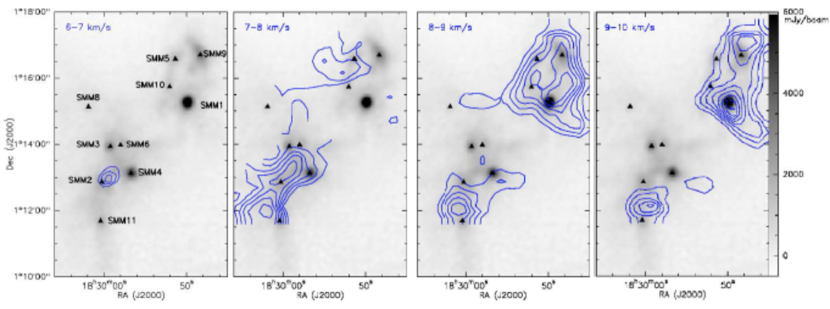
Figure 2: Contour maps of C¹⁷O J=1$\rightarrow$0 modelled emission from the hyperfine fit, overplotted on SCUBA 850$\mu$m emission in gray scale. The submillimetre sources are identified on the left figure with labels and triangles. These symbols will be used from this point forward. Each figure represents a mean intensity map over 1 kms^-1 intervals, from 6 to 10 kms^-1. Contours range from 0.4 K kms^-1 increasing by steps of 0.1 K kms^-1 (in T${}_{\mathrm{A}}^{*}$ scale). The figure shows the SE sub-cluster with three main peaks: one above SMM11, one between SMM2 and SMM6, and finally, one west of SMM4. While the NW sub-cluster also contains three major peaks: one on SMM1, one close to SMM9, and another one south-west of SMM1.

The C¹⁷O J=1$\rightarrow$0 line comprises three, partially blended, hyperfine features. By fitting the hyperfine structure (HFS) of the spectrum, the line width, velocity and optical depth ($\tau$) can be extracted. The line shape in the presence of hyperfine structure can be described by

$$T(v)=T_{S}(1-e^{-\tau(v)}),$$ (1)

where

$$\tau(v)=\tau_{0}\sum^{3}_{i=1}r_{i}\exp\biggl{(}{-\frac{(v-v_{0,i})^{2}}{2\sigma^{2}}}\biggr{)},$$ (2)

$T(v)$ is the line brightness temperature, $T_{S}$ is the source temperature and $\tau$ is the optical depth. The optical depth is the sum over the three hyperfine components of the transition with $r_{i}$ and $v_{o,i}$ - the relative weight and the central velocity for each hyperfine component - being $v$ the velocity, $\sigma$ the velocity dispersion and $\tau_{0}$ the total optical depth common to the three components (Fuller & Myers, 1993). The spacing and weight of the hyperfine components were adopted from Ladd et al. (1998). Further details about the hyperfine structure fitting procedure in the GILDAS software can be found on the IRAM website.

To fit this hyperfine structure, the individual spectrum at each pixel in the image was extracted from the datacube and was fitted using the procedure described above. A model Gaussian spectrum for each pixel was then reconstructed using the derived values (the peak intensity, line width and central velocity). Only pixels where both the line width and line peak intensity were determined with a signal to noise ratio of 5 or greater were considered.

The initial fitting showed that within the uncertainties, all the emission was consistent with being optically thin. Therefore, to reduce the uncertainties on the fitted quantities, the HFS fitting was redone fixing the $\tau$ at 0.1 for the whole map, consistent with optically thin emission. In the final C¹⁷O J=1$\rightarrow$0 modelled datacube (Fig. 2) we were able to identify clear peaks at different velocities and positions in the region. A detailed study of these peaks is presented in Section 3.1.

2.1.2 C¹⁸O

The Serpens C¹⁸O emission is not affected by the outflows in the region (Section 4.1) and the C¹⁸O lines have no hyperfine structure. Therefore, on some regions of the mapped cloud such as the NW sub-cluster (Fig. 1), lines are well represented by a single Gaussian (Fig. 3 left panel). However, in the SE sub-cluster, the line profile has two clear peaks (Fig. 3 lower panel). The low optical depth of the C¹⁸O emission (Section 2.1.1 and 5) together with double peaked lines in this region in other optically thin tracers such as N₂H⁺ J=1$\rightarrow$0 (Olmi & Testi, 2002) suggests that these two peaks trace two clouds along the line of sight towards this sub-cluster. In the weaker C¹⁷O emission with its blended hyperfine structure, these two velocity components are too difficult to separate. However, since it is optically thin, the C¹⁷O emission is still a reliable tracer of the total column density.

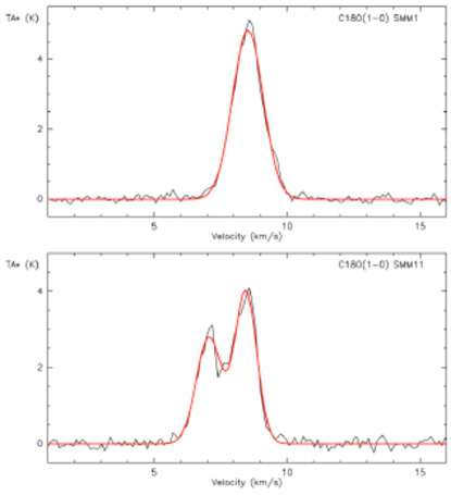
Figure 3: Observed C¹⁸O J=1$\rightarrow$0 spectra (black solid line), smoothed in velocity to 0.1 kms^-1 width channels, at two different positions: on SMM1 (top) and on SMM11 (bottom); with the respective Gaussian fit (red line). These are examples of a single peaked spectrum as seen in the NW sub-cluster and a double peaked profile, as seen in the SE sub-cluster.

2.2 JCMT data

Our excitation analysis (Section 4) makes use of JCMT HARP data from the Gould Belt Survey (GBS) at JCMT (Graves et al., 2010; Ward-Thompson et al., 2007). The data used is C¹⁸O J=3$\rightarrow$2, at 329.330 GHz, with 0.055 kms^-1 spectral resolution, and $14^{\prime\prime}$ spatial resolution. The telescope main beam efficiency at this frequency is $\eta_{\mathrm{mb}}=0.66$ (Curtis et al., 2009), and the rms level achieved is of the order of 0.2 K (T_A). A full description of these data is given in the GBS Serpens First Look paper (Graves et al. 2010, hereafter referred to as SFLPaper).

The submillimetre continuum data at 850 $\mu$m was observed with SCUBA at the JCMT, with a beam size of $14^{\prime\prime}$. The initial reduction, analysis and discussion of these data was presented by Davis et al. (1999), where they estimate the overall dust properties and characteristics of the cloud (see Section 1). We have used the pipeline reduced SCUBA data from the Canadian Astronomy Data Centre (CADC) archives to investigate the structure of the dust continuum emission and for comparison with the IRAM 30m C¹⁷O and C¹⁸O data.

An initial inspection of the SCUBA data indicated good agreement in the source positions for those sources where Davis et al. determined positions from this same SCUBA data (SMM8 and SMM11) and as well as for SMM3. However, in agreement with interferometric continuum observations (Hogerheijde et al., 1999), the positions of some of the remaining SMM sources needed to be revised compared to those listed in Davis et al. (1999) with absolute offsets from the published positions greater than $5^{\prime\prime}$ for SMM2 and SMM6. Table 1 presents redetermined positions for all sources, extracted from the 850 $\mu$m map of Serpens, which now agree within 1^′′ of the positions in the SCUBA cores catalogue published by Di Francesco et al. (2008). We estimate that these positions are accurate within the 2^′′ SCUBA pointing errors (Davis et al., 1999). The offsets in RA and Dec between the revised positions and those previously published (listed in Davis et al., 1999) are also shown on Table 1.

3 Gas structure of the cloud

To determine the structure of the molecular gas we have carried out a clumping analysis in 2D and 3D. Using the velocity information from the gas emission it is possible to identify the individual clumps within the cloud. These are compared to the structure visible in the dust continuum. We use this analysis to quantify the sizes and masses of molecular gas associated with protostars, and carry out a virial analysis to determine the clump stability.

3.1 C¹⁷O 2D-Clumps

Initially we manually extracted the small scale molecular structures for comparison with the dust seen in the SCUBA map. This was done based on a visual inspection of both channel and integrated intensity maps (e.g. Fig. 2). The C¹⁷O J=1$\rightarrow$0 channel maps show a significant number of emission features which are not directly associated with the SCUBA cores. For this reason we call these molecular structures “clumps” although this term is often used to describe parsec-scale structures (Blitz, 1993).

Table 2: Properties of the 2D-clumps

2D-Clump	RApeak	Decpeak	Vpeak	Area	FWHM	Mcf	Mvirial	Ratio	$I_{\mathrm{low}}$     $I_{\mathrm{peak}}$
ID	(J2000)	(J2000)	(kms-1)	(arcmin2)	(kms-1)	(M⊙)	(M⊙)	(Mvirial/Mcf)	(K kms-1)
A	18:29:49.89	01:15:15	8.61	2.30	1.1	9.0	9.3	1.0	1.15     2.42
B	18:29:48.43	01:17:04	8.55	1.83	1.1	5.4	8.3	1.5	0.90     1.90
C	18:29:46.97	01:14:31	8.65	1.33	1.4	4.7	12.9	2.7	1.10     2.17
D	18:29:55.43	01:16:25	7.73	0.98	1.3	1.9	11.8	6.2	0.50     0.74
E	18:29:59.40	01:13:04	7.43	1.00	2.2	2.0	25.2	12.6	0.60     1.99
F	18:30:00.87	01:11:58	8.29	1.63	1.8	7.1	23.4	3.3	1.35     2.89
G	18:29:55.75	01:12:53	8.36	0.70	1.4	1.6	8.5	5.3	0.90     1.33
NW	18:29:49.89	01:15:15	8.61	9.06	1.2	31.3	33.2	1.1	1.00     2.42
SE	18:30:00.87	01:11:58	8.29	7.49	1.9	26.0	70.3	2.7	1.00     2.89

The properties of each identified clump (Fig. 4) was subsequently extracted using the IDL 2D version of the source extraction clumpfind algorithm code by Williams et al. (1994) on maps integrated over the velocity range in which each clump appeared.

With the size and the integrated intensity corrected for telescope efficiency, we estimated the column density and mass of each clump (M_cf) assuming a temperature of 10 K, a mean molecular weight of 2.33 and a C¹⁷O fractional abundance with respect to H₂ of 4.7 $\times$ 10^-8 (Frerking et al., 1982; Jørgensen et al., 2002). We also calculated the clumps virial masses using Eq. 3, where $M_{\mathrm{vir}}$ is the virial mass, $\sigma_{\mathrm{obs}}$ is the observed velocity dispersion, $G$ is the gravitational constant and $\alpha$ is a coefficient function of the adopted density profile: $\alpha$ is 3/5 for a uniform density, 2/3 for a profile as $\rho\propto r^{-1}$, 3/4 when $\rho\propto r^{-1.5}$, and 1 when $\rho\propto r^{-2}$.

$$M_{\mathrm{vir}}=\frac{3R\sigma_{\mathrm{obs}}^{2}}{\alpha G}$$ (3)

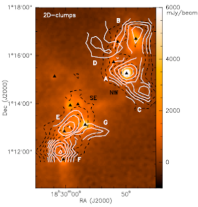
Figure 4: SCUBA map of the 850 $\mu$m continuum emission (colour scale) overplotted with the positions of the submillimetre sources (triangles), the C¹⁷O J=1-0 2D-clumps (solid white contours and letters) and the NW and SE sub-clusters (black dashed contours). The solid white contours are the intensity integrated over the correspondent velocity range for each clump. These are stepped by 0.2 K kms^-1, except for weaker 2D-clumps G and D, stepped by 0.1 K kms^-1 (in T${}_{A}^{*}$). The lower level of each clump is the same as the specified on Table 2. The NW and SE sub-clusters contours are integrated intensity over the entire velocity range. Contours are stepped by 0.25 K kms^-1, with the lower contour at 1.25 K kms^-1 (in T${}_{\mathrm{A}}^{*}$).

The listed virial masses of the clumps adopt a density profile of $\rho\propto r^{-2}$. The velocity FWHM of each clump was estimated by averaging all the spectra assigned to that clump and has an estimated uncertainty of $\sim$0.1 kms^-1. The clumps identified by this method will be referred to as the 2D-clumps hereafter.

The virial mass (M_virial) and the gas mass (M_cf) were also calculated for the two sub-clusters, NW and SE. The method was the same as for the clumps except the density profile for the sub-cluster gas was assumed to be $\rho\propto r^{-1.5}$, which is expected to be more appropriate for these larger size regions. If the same $\rho\propto r^{-2}$ as for the clumps had been adopted, the derived sub-cluster mass would be a factor of 25% smaller.

The clumps are shown on Fig.4, and the physical parameters summarized on Table 2, where: RA_peak and Dec_peak are the position where the emission peaks within each clump; V_peak is the velocity at the peak position, with an uncertainty of 0.05 kms^-1; area is the surface in the map occupied by each clump; M_cf is the mass of the clump calculated from clumpfind outputs; M_virial is the virial mass; Ratio M_virial/M_cf is a measurement of how bound each clump is - a gravitationally bound structure should have a ratio around unity, but given the uncertainties of these calculations, we consider a structure to be unbound if the ratio is above 2; I_low represents the lower contouring level assumed when running the algorithm for each different clump (increasing with steps of 0.10 K kms^-1); and, finally, I_peak shows the integrated intensity in T${}_{\mathrm{A}}^{*}$as measured at the peak position.

Observational sources of uncertainty include the distance to Serpens and the line width. Uncertainties on the line width in particular might be a special issue in the SE region where the two velocity components observed in C¹⁸O may become important in broadening the C¹⁷O line. Systematic uncertainties in M_cf include uncertainty in the adopted gas temperature and fractional abundance of C¹⁷O. Finally, the systematic uncertainties on the M_virial include source geometry effects and the neglection of additional terms in the virial equation (due to external pressure, magnetic pressure, etc.). Amongst all the possible sources of uncertainty, the greatest is likely to be the factional abundance of C¹⁷O, given that our non-LTE study of C¹⁸O at 8 positions (Sec. 5) show a mean depletion factor of 2.5 (App. B). Given the observational and possible systematic uncertainties on the calculations, the virial ratio is perhaps best seen as a useful tool to compare the different structures within a cloud rather than absolute measure of the gravitational equilibrium of any given clump.

The NW and SE sub-clusters are extended regions, and therefore, the peak positions and velocities correspond to one of the smaller identified clumps lying within the sub-cluster. The NW sub-cluster peaks at the position of clump A (& SMM1) and the SE sub-cluster peaks at the position of clump F (north of SMM11). Similarly, the velocities quoted for the peak for the sub-clusters are not the mean velocity of the sub-clusters, but the velocity at the peak of the strongest clump.

Note that even though both sub-clusters, SE and NW, have similar masses (M_cf), they each have a different equilibrium status, with a factor of 3 difference between their respective virial ratio. Interestingly, even when considering some depletion (Appendix  B), the SE region is likely super-virial whereas the NW, due to its smaller line width, is marginally sub-virial. About 67% of the mass in the NW region and 40% of the mass in the SE region is associated with the clumps. Four of the clumps (A, B, C and F) are individually within a factor of three of being in virial equilibrium. Accounting for some depletion of C¹⁸O (Appendix  B), M_cf could increase up to a factor of 2.5, which would make all these four clumps relatively bound structures. Clump D is a factor of $\sim 6$ super-virial, and is likely to be less affected by depletion as the dust densities are lower, likely identifying this clump as part of a more diffuse region which is less bound than the NW sub-cluster. Finally, even accounting for possible depletion, clumps, E and G, with mass ratios of $\sim 13$ and $\sim 5$, are likely unbound structures. They may either represent shocked regions where the line width is intrinsically high (from 1.6 to 2.2 kms^-1) or regions where, as mentioned in section 2.1.2, two blended velocity components contribute to the emission along the same line of sight. The HFS fitting of a single component in this case would result in a broadening of the line width due to blending of the two components. However, in Sec. 4.3 we see that even after separating the components, the line width of at least one of them is still broader than seen anywhere in the NW, pointing to a genuine broad line emission. In summary, the SE sub-cluster is much more dynamic than the NW, with a kinematic support a few times higher, both when comparing individual clumps and the overall sub-clusters.

3.2 C¹⁷O 3D-Clumps

Although the 2D clumpfinding is valuable for comparison with the dust continuum, it is limited in its ability to represent the true structure of the cloud. The 3D clumpfind automatically studies the datacube in all three dimensions of space-space-velocity. In particular, 3D clumpfind should provide a better understanding of the cloud’s structure where clumps may overlap along a line of sight but have different velocities, or where the emission is narrow in velocity making it weak in integrated intensity maps. Therefore we have complemented the 2D study of the structure of the C¹⁷O using the 3D version of the clumpfind within the Starlink package.

Table 3: Properties of the 3D-clumps

3D-clump	RApeak	Decpeak	Vpeak	Area	FWHM	Mcf	Mvirial	Ratio	Tpeak
ID	(J2000)	(J2000)	(kms-1)	(arcmin2)	(kms-1)	(M⊙)	(M⊙)	(Mvirial/Mcf)	(K)
1	18:29:51.0	1:15:04	8.64	3.93	1.0	9.0	10.5	1.2	2.0
2	18:29:49.2	1:16:09	8.56	3.46	1.4	7.3	20.0	2.7	1.6
3	18:30:01.6	1:11:47	8.67	2.30	2.0	6.3	31.2	4.9	1.3
4	18:29:49.2	1:09:57	8.20	1.43	0.3	0.6	0.4	0.7	1.1
5	18:29:47.0	1:13:58	8.80	1.53	1.2	2.5	9.1	3.6	1.0
6	18:29:55.0	1:12:41	8.51	1.13	1.1	1.3	6.4	4.9	0.9
7	18:30:10.3	1:13:25	8.09	1.00	0.4	0.6	1.0	1.7	1.1
8	18:29:44.8	1:17:04	8.80	1.77	0.9	1.2	5.3	4.4	1.1
9	18:29:47.0	1:09:24	8.41	0.73	0.4	0.3	0.6	2.0	1.0
10	18:30:00.1	1:12:52	7.68	1.13	1.5	1.6	13.7	8.6	0.8
11	18:29:58.7	1:15:04	8.23	0.73	0.9	0.8	4.0	5.0	0.8
12	18:30:06.0	1:11:58	7.36	1.07	1.2	0.8	8.4	10.5	0.7
13	18:29:57.9	1:15:48	7.88	1.67	0.6	0.7	2.6	3.7	0.7
14	18:29:57.2	1:11:47	8.67	0.90	0.8	0.4	3.0	7.5	0.7
15	18:29:55.7	1:16:20	7.73	1.37	0.8	0.6	3.9	6.5	0.8
16	18:29:47.0	1:11:48	8.80	0.93	0.3	0.2	0.3	1.5	0.7

Similarly to Pineda et al. (2009), we also found that the results on the 3D clumpfind analysis to be very sensitive to the parameters used, especially in characterising the weaker emitting regions. Stronger clumps were unequivocally detected with a wide range of parameters, but changing the step size and/or the number of pixels per clump allowed to be adjacent to a bad pixel would result in the merging of several clumps into one, or unrealistic extensive splitting of clumps into several small structures, or even non-detection of some structures expected to be detected. For this reason, the initial 2D study is essential as a reference point to understand the main structure of the cloud, which could be significantly misrepresented by relying, uncritically and exclusively on the 3D clumpfind analysis. The best configuration parameters we found for this analysis were: the first contour level, $\mathrm{T_{low}}$, of 0.6 K; the global noise level of the data, r.m.s., of 0.2 K; and the spacing between the contour levels, $\mathrm{\Delta T}$, of 0.05 K.

This analysis identified a total of 16 clumps which will be called the 3D-clumps hereafter. These clumps are shown on Figure 5 as integrated intensity maps in T${}_{\mathrm{A}}^{*}$.kms^-1 plotted over the continuum 850 $\mu$m data from SCUBA. Table 3 shows the properties of the 3D clumps as numbered and plotted on Figure 5. The nine first columns are as in Table 2 the last column being the intensity at the peak position in T${}_{\mathrm{A}}^{*}$. Once again, masses were calculated after correcting for the IRAM 30m telescope efficiency for the C¹⁷O J=1$\rightarrow$0.

Due to the difficulty in interpreting partial spectra split by 3D clumpfind between multiple spatially coincident clumps, the mean line width of the 3D-clumps was recovered using a different approach to that used for the 2D-clumps. The velocity dispersion, $\sigma$, of each clump was estimated by determining the velocity range where the emission of the clump was above $e^{-1/2}$ of its peak intensity. This was done by visually inspecting these thresholded channel maps of each clump. The quoted FWHM is $2.35\leavevmode\nobreak\ \sigma$ and has an estimated uncertainty of 0.1 kms^-1, twice the uncertainty of the peak velocity, 0.05 kms^-1.

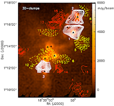
Figure 5: SCUBA map of the 850 $\mu$m continuum emission (colour scale) overplotted with all the C¹⁷O J=1-0 3D-clumps integrated intensity maps (contours and numbers). The numbering of the cores is based on their peak intensity. The different contour style and colours identify clumps starting at different contour levels. The white solid contours are the clumps with the stronger integrated emission, with contours starting at 1 K kms^-1, the dashed yellow contours start at 0.3 K kms^-1, and the solid red contours start at 0.1 K kms^-1 step. For all clumps, the contour step is 0.1 K kms^-1.

The mass of the clumps within the NW sub-cluster inferred from the size and integrated intensity of 3D-clumps 1, 2, 5 and 8 correspond to about 65% of the total mass of that sub-cluster. Including clumps number 11, 13 and 15 in this calculation, the fraction of gas-mass in the clumps rises to 70%. The 3D-clumps 3, 6, 10, 12 and 14 constitute 40% of the mass of the SE sub-cluster. This is consistent with the results from the 2D-clumps.

Since the velocity structure in the region can affect the deduced clump structure, we also experimented with 3D clumpfind on the C¹⁸O J=1$\rightarrow$0 data. The results from this differed from those of C¹⁷O only in that two clumps (3D-clumps 3 and 10) were subdivided into 2 and 3 sub-clumps respectively. Collectively, these sub-clumps had properties very similar to their respective C¹⁷O clumps. The presence of these possible sub-clumps does not significantly alter the interpretation of the region for the purpose of our analysis, indicating that the C¹⁷O clumps adequately describe Serpens.

3.3 Structure of the region: combining information from 2D and 3D-clumps

The north region has two clear clumps unequivocally identified in both 2D and 3D methods: 2D-clumps A and B, which correspond to 3D-clumps 1 and 2 respectively. Both peak close to the position of the strongest submillimetre sources in this region (SMM1 and SMM9), and trace the gas around them in good agreement to the cold dense dust traced by the 850 $\mu$m emission.

A region with higher velocity gas was detected with the 2D analysis as 2D-clump C which corresponds to 3D-clump 5. This region has quite strong integrated emission making it detectable in the 2D search. However, as it peaks at a very similar velocity to clump 1/A, the 3D search failed to separate these two in some of our trial runs of the 3D analysis. This clump is associated with very little submillimetre continuum emission but quite strong C¹⁷O (and C¹⁸O) emission. The fact that it is also seen in N₂H⁺ (Olmi & Testi, 2002) and not in ¹²CO tracing outflows (SFLPaper), is consistent with the possibility of this being a denser region, close to being bound, directly associated with the NW sub-cluster. It could, for example, be a very young prestellar core about to become gravitationally unstable and collapse (Walsh et al., 2007).

A region detected with the 3D analysis which was not seen in the 2D search was 3D-clump 8. This clump is detected at high velocities (8.8 kms^-1) and seems to surround the clump 2/B associated with SMM9, perhaps as a shell. Although apparently somewhat super-virial clump, if affected by a depletion of C¹⁸O by a factor of 2-3 (Appendix  B), this clump could be gas undergoing gravitational collapse.

Finally there is also a low velocity region situated at the left of the main clumps of the NW sub-cluster - detected as a single clump with the 2D method (clump D, on Fig. 4) and as three separate clumps with the 3D clumpfind (11, 13 and 15 on Figure 5). This region has a very small mass ($\sim$ 1 - 2 M_⊙) and is about 5 times super-virial. It seems to be a quiescent region at lower velocities than the main cloud and connecting to the main cloud very close to the edge of the NW sub-cluster as seen on dust emission.

The bulk of emission on this NW sub-cluster presents a very coherent structure in space and velocity throughout. It does not appear to be as filamentary as the SE sub-cluster and the emission appears confined to relatively dense, cool compact regions.

The SE sub-cluster is quite different from the NW cluster, both in spatial structure and velocity, even though this is not obvious from the dust emission. Note the higher virial ratios for the clumps within the SE sub-cluster, when compared to the ones in the NW, supporting once again the idea of more kinetic support in the south, even when the 3D velocity-separated clumps are considered. Comparing the 2D and 3D results, shows the C¹⁷O emission is more complex with none of the gas emission peaks coincide with any of the compact submillimetre sources. The main peaks of the C¹⁷O emission in this region lie in the filament seen in dust continuum emission, between the compact sources. The 2D-clumps E and F were detected as 3D-clumps 10 and 3 respectively. However, the 3D search found a more diffuse clump, 3D-clump 12, which peaks east of the filament but with its edges still overlapping spatially with 3D-clump 10 and 3, having lower velocities than these two: 7.36 kms^-1 of clump 12, versus 7.68 kms^-1 and 8.67 kms^-1 of clump 10 and 3 respectively. Despite being adjacent, and with overlapping edges, 3D-clumps 3 and 10 have a difference of 1 kms^-1 between their peak velocities. There is a similar velocity difference between clump 10 and clump 6, west of the filament: 3D-clump 6, detected in the 2D analysis as 2D-clump G, has a peak velocity of 8.51 kms^-1, $\sim$0.8 kms^-1 higher than its neighbour. These four 3D-clumps (3, 6, 10 and 12), with two sets of different peak velocities (at $\sim$7.5 kms^-1 and $\sim$8.5 kms^-1), overlap with each other at low intensities mainly throughout this filamentary structure of the SE sub-cluster, even though their emission peaks are spatially offset. This also shows that the double velocity structure in the SE sub-cluster (Section 2.1.2) is to some extent, recoverable from a single line fit using a 3D clumpfind analysis.

The remaining clumps detected in the SE sub-clusters trace the less dense gas around this main filament. These were not detected in the 2D search mainly due to their very narrow line widths, between 0.3 and 0.5 kms^-1, making them faint in integrated intensity maps. Note that the dominant emission detected east of the filament has lower velocities (3D-clump 7 has a peak velocity of 8.09 kms^-1), whereas the regions detected to the west have higher velocities (3D-clumps 4, 9 and 16), with mean velocities from 8.20 kms^-1 to 8.80 kms^-1.

Globally, there appears to be a velocity gradient from east to west of nearly 1 kms^-1 over slightly more than 0.1 pc. However, this is not a smooth gradient throughout, as in the filamentary structure there are spatially-overlapping clumps with very different velocities. This velocity structure is further investigated using the C¹⁸O lines, which are not split by hyperfine structure in Section 4.2.

4 Dynamics of the cloud: velocity and line width

4.1 Outflows

One important issue when studying gas dynamics in regions of active star formation is the extent to which the line widths of molecular species are influenced by outflows. Using the available data, we looked for the influence of outflows on the size scale of the cores by investigating the spectra associated with all the submillimetre sources, looking for possible wing emission.

Although wings on C¹⁸O lines have proven to be able to trace outflow interaction (Fuller & Ladd, 2002), in Serpens and with the 0.45K rms noise of our dataset (Section 2.1) no wings were found. The lines towards sources with known outflows are well fitted by a single Gaussian. For example, Fig 3 (top panel) shows the C¹⁸O towards SMM1, a source known to have an outflow, e.g. Hurt & Barsony 1996, is well represented by a single Gaussian component. In the SFLPaper, we have also searched for evidence of the influence of outflows in the C¹⁸O emission by comparing the C¹⁸O J=3$\rightarrow$2 emission to the ¹²CO J=3$\rightarrow$2 emission tracing the outflows. No correlation nor anti-correlation between the C¹⁸O emission and the outflows is found in the region. Both these approaches lead us to conclude that the Serpens C¹⁸O emission is not influenced by outflows and, therefore, the velocity components we detect in C¹⁸O are related to the global cloud dynamics.

4.2 Position - Velocity structure

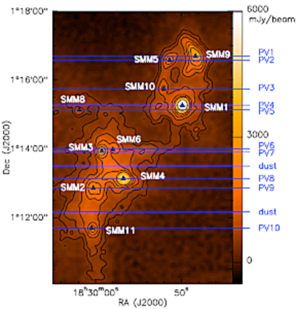
Figure 6: SCUBA 850 $\mu$m map of Serpens in colour scale and contours (contours as in Fig.1), showing the cuts used for the position-velocity diagrams of C¹⁸O J=1-0 emission (Fig. 7, 8 and 9). The cuts made crossing the SMM sources are denoted as PV#, where # is the number of the cut, starting from the north. There are two cuts which are denoted as “dust” which do not intercept any source, but were made to understand the velocity structure around the dust filament.

PV1

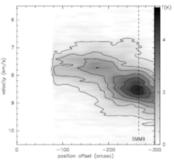
PV2

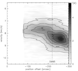
PV3

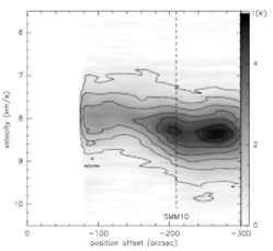
PV4

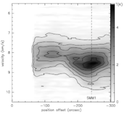
Figure 7: Position-velocity diagrams of the C¹⁸O J=1$\rightarrow$0 emission. The cuts are horizontal slices of the map, as shown in Fig. 6. The sources name and RA position are indicated in each figure (dashed line). The declinations are presented in Table 1 and the RA varies from $18^{h}$$30^{m}$$06^{s}$ to $18^{h}$$29^{m}$$46^{s}$ (from 0 to -300 ^′′ offset respectively). The gray scale shows the line intensity in T${}_{\mathrm{A}}^{*}$.

PV5

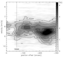
PV6

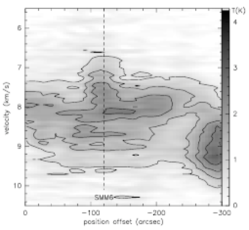
PV7

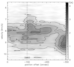
dust

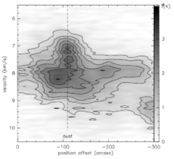
Figure 8: Same type of position-velocity diagrams as Fig.7 for the SE sub-cluster. The RA also varies from $18^{h}$$30^{m}$$06^{s}$ to $18^{h}$$29^{m}$$46^{s}$ (from 0 to -300 ^′′ offset respectively). PV diagrams displayed in descending declination, as they appear on Fig. 6.

PV8

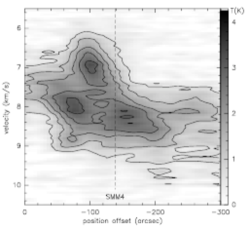
PV9

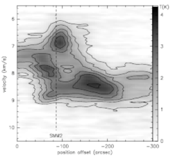
dust

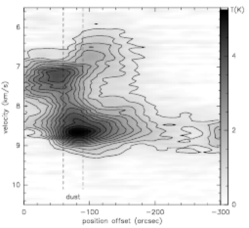
PV10

Figure 9: Fig. 8 continued: remaining position-velocity diagrams of the SE sub-cluster as plotted on Fig. 6.

As revealed by the C¹⁷O (Section 3.1), the NW region is mostly traced by higher velocity emission, the exception being the region offset to the east of the sub-cluster. On the other hand, the SE is not so homogeneous, containing both higher and lower velocity components, which overlap approximately where the filamentary structure is seen in the continuum observations. The C¹⁸O shows very well defined double peaked emission along the southern region, that starts disappearing as we move north. Figure 3 shows two examples of spectra in this region, and Fig. 9 shows the evolution of the double component along the map. The existence of a double-peaked spectrum in other optically thin tracers such as N₂H⁺ (Olmi & Testi, 2002) rules out self absorption as an explanation of the double peaked C¹⁸O emission (cf Section 2.1.2).

On the basis of a study of the line centroid velocity (despite the presence of double peaked lines) Olmi & Testi (2002) argued that the region is undergoing global rotation. However position-velocity diagrams of horizontal slices along the C¹⁸O map are incompatible with this interpretation (Fig. 6 and Fig. 7 to 9). Moving from north to south, and slicing at the declination of each SMM source, we can see the two separate clouds, very well distinguished close to SMM11. For simple rotation, we would expect to see a smooth gradient along the velocity axis as the RA changes. Instead we observe two velocity components, clearly separated in the southern part of Serpens (see e.g. PV10) and merging together when moving to the north of the sub-cluster (see e.g. PV7). At this point, the two components are barely distinct lines, producing broad, non-gaussian profile. Furthermore, the SMM sources in the SE sub-cluster appear at the edges of the double velocity region (hereafter referred to as the interface), whilst the filamentary structure seen in dust follows the interface region itself (see the PV diagrams labeled as “dust” on Fig. 8 and 9).

The lower velocity cloud (hereafter LVC) appears to be interacting with the high velocity cloud (hereafter HVC), apparently provoking the enhanced dust emission between SMM2, SMM3, SMM4 and SMM6 - and also the elongated filament that extends south towards SMM11 and beyond. A dynamical interaction between two clouds, as indicated by this space-velocity structure and the turbulent motions found towards the south, might have triggered this episode of star formation along the filament (Sec. 6).

4.3 Decomposition of the C¹⁸O line components

To investigate the velocity structure of the C¹⁸O J=1$\rightarrow$0 emission we have decomposed the datacube in two, by fitting two velocity components to the C¹⁸O spectra and then creating a model datacube from the Gaussian fits, for each of the two components. The results of this decomposition are shown in Fig. 10 and Fig. 11.

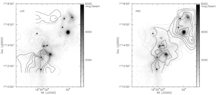
Figure 10: Integrated intensity maps as a result of the separation of the two line components of the C¹⁸O J=1-0 transition, under the assumption of two different clouds seen along the line of sight. The LVC is shown on the left and HVC on the right. The background grey scale shows the 850 $\mu$m emission tracing the cold dust, with its respective submillimetre sources plotted as triangles. The contours represent the integrated intensity of the modelled Gaussians (fitting the data in T${}_{\mathrm{A}}^{*}$). Contour key: left (LVC) at 0.2 K kms^-1 (dashed) and 1.5, 2.5, 3.2 and 4.0 K kms^-1 (solid); right (HVC) at 2.5 and 3.0 K kms^-1 (dashed) and 3.2, 4.0, 5.0, 5.5 and 6.0 K kms^-1 (solid).

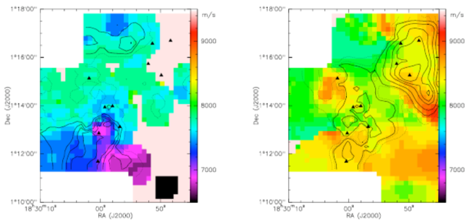
Figure 11: Velocity structure maps of Serpens, as a result of the separation of the two line components of the C¹⁸O J=1-0 transition. As in Fig. 10, the LVC is represented on the left and HVC on the right. The submillimetre sources are plotted as triangles, and the contours represent the integrated intensity as in Fig. 10. The colour scale is now the centroid velocity of the same modelled Gaussians, where the light pink colour represents the lack of a fit to that velocity component.

The data were first rebinned to 0.1 kms^-1 velocity channels. Then, for each spectrum, the line was fitted with a single Gaussian and then a double Gaussian. The two Gaussian fit was selected as the model for the line only if: i) the difference between the central velocities of the two Gaussian fit ($\Delta V$) was greater than 0.35 kms^-1 or ii) both lines were relatively strong with the peak intensity ratio of the stronger to the weaker line less than 2.4. The value of 2.4 was determined by a careful analysis of various line fits which showed that if the ratio was more than 2.4, the weaker line fit was poorly fit. The remaining spectra were fitted with a single Gaussian. An example of this fitting is shown on Figure 3 (lower panel). From this fitting procedure, two model datacubes were created, one for each velocity component, allowing us to study the two clouds separately. The higher velocity component (HVC) of the double peaked lines, as well as the single lines with central velocity greater than 7.8 kms^-1, were included in the HVC datacube; lower-velocity lines and single lines peaking below 7.8 kms^-1 were incorporated in the LVC model datacube.

Figure 10 shows the spatial distribution of the LVC and HVC using the integrated intensity from the model datacubes. Overall, the HVC traces the distribution of the 850 $\mu$m continuum emission better than the LVC. The HVC emission is stronger in the north, but it lies along the filament containing both sub-clusters, extending roughly in a SE-NW direction. The LVC is roughly aligned along the S-N direction and is stronger in the south, where it meets the HVC.

Figure 11 shows again the integrated intensity of the modelled datacubes for each component, but shows also the velocity structure of each cloud. In the NW sub-cluster, the HVC appears at velocities around 8.4 kms^-1, with the exception of a few regions at the edges of the cloud, which appear to reach velocities as high as 8.8 kms^-1. The region which stands out from the bulk of this sub-cluster is the region SW of SMM1, which is not present in the dust emission even though it is rather strong in gas emission, having the highest velocities of the entire cloud (reaching 9 kms^-1). The LVC, in the NW sub-cluster, is spatially offset to east, with velocities of 7.5 - 7.8 kms^-1, similar to most of the emission in the south.

The region between the two sub-clusters, dominated by the emission from the HVC, has the systemic velocity of Serpens (around 8.0 kms^-1) possibly due to the merging of the two components. Note that the emission here is rather weak, and the presence of SVS2, a more evolved (flat spectrum) near-IR source (Kaas et al., 2004), suggests this region may be more evolved.

In the SE sub-cluster, the HVC velocities range from 8 and 8.5 kms^-1, being higher towards the southern end of the filament. On the other hand, the LVC shows a velocity gradient increasing from west to east - contrary to the HVC. The material west of the southern filament, has velocities of about 6.8 - 7 kms^-1. At the centre of the filament the velocities are around 7.5 kms^-1, translating into a gradient of $\sim$ 5 kms^-1pc^-1. To the east of the filament the velocities are approximately constant and around 7.5 kms^-1. Therefore, it seems that the clouds have a greater offset in velocities in the far-south end of the filament, converging into one intermediate velocity as one moves north. When two lines can no longer be separated, the emission becomes a single broader line, centered at the intermediate velocities ($\sim$ 8 kms^-1).

The line width in the SE sub-cluster, specially where the two components merge, is around 2 kms^-1. This is almost twice the line width of the NW ($\sim$ 1 kms^-1). This difference is reflected as a four times higher kinetic support in the SE region, in comparison to the NW region. This is consistent with the C¹⁷O J=1$\rightarrow$0 analysis (Section 3.1), where it was showed that the NW sub-cluster is a bound structure, whereas the SE sub-cluster was somewhat super-virial. The SE is therefore much more dynamic than the NW, as already foreseen by the C¹⁷O analysis.

5 Physical properties: Temperatures and column densities

The optical depth of the C¹⁸O can be estimated from the ratio of the integrated intensities of the C¹⁸O and C¹⁷O J=1$\rightarrow$0 transitions. Over the mapped region the observed ratio shows little coherent spatial structure and is approximately constant with a value consistent with the abundance ratio of the species, $\sim$3.5 (e.g. Penzias, 1980; Frerking et al., 1982) implying the emission from both species is optically thin.

To better understand the correlation between the dust and gas in this region, Figure 12 shows a pixel-by-pixel comparison of the 850 $\mu$m flux density against the integrated intensity of the three transitions of C¹⁸O, all convolved to a common resolution of 24^′′. For the purpose of these scatter plots, we have oversampled the data to a pixel size of $2.5^{\prime\prime}$, in order to better distinguish the trends.

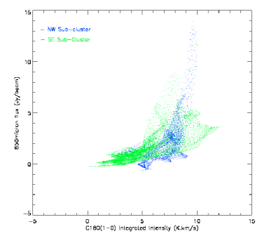
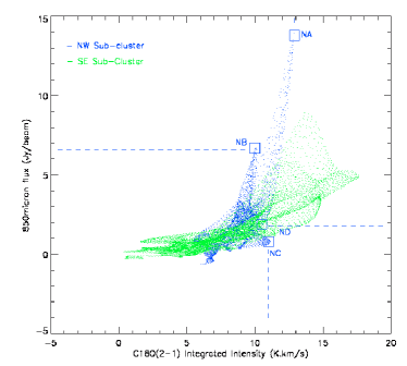
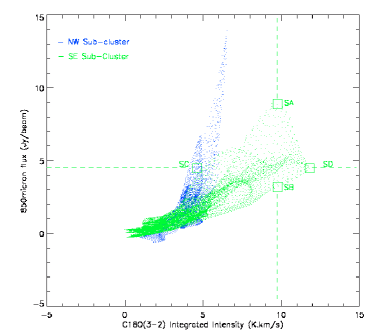
Figure 12: Scatter plots of the SCUBA 850 $\mu$m dust emission against the C¹⁸O integrated intensity over the whole range of velocities (top: J=1$\rightarrow$0, middle: J=2$\rightarrow$1, bottom: J=3$\rightarrow$2). Blue points show the NW sub-cluster and green points the SE sub-cluster. The four positions chosen in each sub-cluster to investigate with non-LTE modelling shown on the middle panel for the NW region and the lower panel for the SE region. These positions are also indicated on Fig. 13.

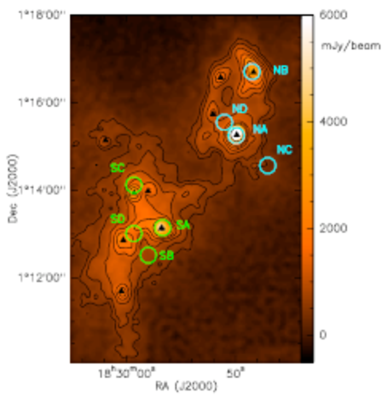
Figure 13: Map showing the positions of the selected regions for the non-LTE RADEX study indicated by blue and green circles (for the positions in the NW and SE sub-clusters, respectively) and labeled as in Fig. 12. The contours and colour scale show the SCUBA 850 $\mu$m emission as in Fig. 6.

Overall, the distribution of points is very similar for the three transitions. There is a general correlation between dust and gas, especially for the weaker emission (Fig. 12). However, the distributions also show structure which consistently appears across all three transitions. The very prominent peaks of dust emission corresponding to the stronger submillimetre sources are obvious, and although in general there is an increase in the C¹⁸O emission at these positions, the dust peaks do not correspond to global peaks in the C¹⁸O emission. Indeed the nature of the relationship between the C¹⁸O emission and the dust appears different in the NW and SE sub-clusters.

Focusing on the NW region (blue in Fig. 12), the plots are dominated by the two dust peaks, each of which is associated with a well defined, but separate, increase in C¹⁸O emission. Comparing the C¹⁸O intensity, the emission becomes weaker moving to higher energy transitions. On the other hand, the SE sub-cluster (green in the figure) shows a different trend from transition to transition, becoming stronger at higher transitions. In addition, there appears to be a more pronounced general correlation in this region between the dust and line emission. Nevertheless, there are clearly structures departing from this trend: several 850 $\mu$m peaks corresponding to SMM sources; and C¹⁸O peaks, which do not have significant submillimetre emission.

5.1 LTE Analysis

From the dust continuum emission, the volume densities in the Serpens sub-clusters are typically higher than the critical densities of each of the three transitions (Table 4) observed here. We therefore initially calculate the gas properties assuming LTE (local thermodynamic equilibrium) using a rotation diagram analysis. Despite its uncertainties, the rotation diagram method is robust in retrieving the column density structure and trends throughout the region, as well as the approximate absolute column densities.

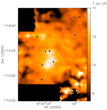
Figure 14: LTE excitation temperature map in colour scale. The dotted black contours show the dust 850 $\mu$m emission at 0.6, 1.2 and 1.8 Jy beam^-1.

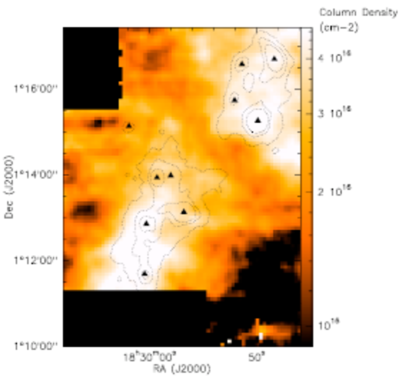
Figure 15: Column density map (colour scale) derived from the rotation diagram method. The dust 850 $\mu$m emission is overplotted in dotted black contours, at the same levels as in Fig. 14.

Table 4: Critical densities (n_critical) at 10K and 20K for C¹⁸O

C18O	Au	Ku	ncritical
transition	(s-1)	(10-11 cm3s-1)	(103 cm-3)
		10K – 20K	10K – 20K
J=1$\rightarrow$0	6.266$\times$10-8	3.3 – 3.3	1.9 – 1.9
J=2$\rightarrow$1	6.011$\times$10-7	7.2 – 6.5	8.3 – 9.3
J=3$\rightarrow$2	2.172$\times$10-6	7.9 – 7.1	27 – 30

These values were derived using the information provided by the Leiden Atomic and Molecular Database (Schoeier et al., 2005): A_u being the Einstein Coefficient for the upper level, and K_u the respective collision rate at both 10 K and 20 K.

Fig. 14 shows a map of the excitation temperature across the region constructed from the 24^′′ resolution integrated intensity maps sampled with 5^′′ pixels (as in the original IRAM data). This shows the NW and SE sub-clusters to have different temperature structures. The NW appears very homogeneous with no significant temperature peaks and with temperatures ranging from 9 to 10 K. In contrast the SE region has both higher temperatures, ranging from $\sim$ 10 to 14 K and a much more peaked distribution. Interestingly, this enhanced temperature in the south does not peak on the SMM protostars but rather between them, along the dust filament which corresponds to the interface region seen on the PV diagrams (Fig. 8 and 9).

The C¹⁸O column density map (Fig. 15) calculated from the rotation diagram recovers more of the dust structure than the temperature map. Both the south and north sub-clusters are evident as denser regions, even though the dust and gas column densities peaks are not always coincident, especially in the SE. The mean C¹⁸O column densities are very similar in the north and the south. The regions with higher gas column density (the entire NW sub-cluster and the filament between SMM11 and SMM2 in the SE sub-cluster) have a lower temperature. Conversely the regions with slightly lower gas column density (between SMM2, SMM4, SMM3 and SMM6 in the SE sub-cluster) have higher temperature. The region south-west of the NW sub-cluster which appears to have a relatively high gas column density seems to have very similar properties to the rest of the NW sub-cluster and yet it is not detected in dust emission.

5.2 Non-LTE Analysis

To better understand the physical conditions of Serpens and the apparent discrepancies between the gas and dust emission, we have selected 4 key positions in the NW and another 4 in the SE using the scatter plots (Fig. 12) for more detailed analysis. The selected positions are indicated on Fig. 13. These positions correspond to interesting features in the correlations between the dust and gas emission, selected to span the range of the correlation. For these positions we performed a non-LTE analysis using RADEX.

We created a $500\times 500$ grid of gas column density (ranging from 10¹² to 10¹⁹ cm^-2) and temperature (ranging from 5 K to 40 K). For each grid point we used RADEX to calculate the C¹⁸O integrated intensities for all three transitions (denoted as $I_{(J_{up}-J_{low})}$). For each position modelled, a volume density determined from the submillimetre dust continuum emission was adopted, assuming a cloud depth of 0.2 pc (based on the projected size of the dust emission), a dust opacity of 0.02 cm²g^-1 at 850 $\mu$m (van der Tak et al., 1999; Johnstone & Bally, 2006) and a dust temperature of 10 K for all but three positions. The three exceptions are: position NA ($\equiv$SMM1) where 38 K was adopted from the SED fit by Davis et al. (1999), and positions NB($\equiv$SMM9) and SA$(\equiv$SMM4), where we adopted a temperature of 25 K, consistent with the $>20$ K determined by Davis et al. (1999). For each of the southern positions, we assumed the H₂ volume density to be the same for both C¹⁸O velocity components. Changing the dust temperature or the assumed cloud depth changes the estimated the H₂ volume densities, however this only becomes important if the derived volume densities becomes lower than the critical densities for our transitions. We have tested these effects using RADEX, and the resulting column densities and kinetic temperatures remain unaffected by changes in the assumed dust temperature between 10 K and 40 K, or in the assumed depth between 0.1pc and 0.3pc. If the transitions are thermalised, only the fractional abundance of C¹⁸O will be affected by changing the assumed H₂ column density.

Table 5: Modelling results for the 8 positions selected from the scatter plots (App. A).

	H2	Line	Central	non-LTE	non-LTE	LTE
Position	volume density	width	velocity	column density	Tkin	Texc
	($\times\leavevmode\nobreak\ 10^{5}$ cm-3)	(kms-1)	(kms-1)	($\times\leavevmode\nobreak\ 10^{15}$ cm-2)	(K)	(K)
NA	2.60	1.6	8.5	15.4	11.7	10.3
NB	2.25	1.5	8.4	11.9	10.6	9.5
NC	1.62	1.9	8.5	11.9	10.5	9.5
ND	6.50	1.4	8.5	13.5	11.4	9.5
SA1	2.98	2.2	7.8	6.4	18.2	13.4
SA2	2.98	1.0	8.3	4.2	6.6
SB1	3.99	1.5	6.9	6.0	11.9	12.7
SB2	3.99	1.1	8.5	4.4	14.8
SC1	6.28	1.7	7.7	5.8	11.7	10.2
SC2	6.28	1.2	8.7	1.4	14.2
SD1	7.81	1.1	6.9	7.3	16.6	12.8
SD2	7.81	1.4	8.2	5.8	14.4

Positions starting with N are in the NW sub-cluster while positions in the southern region start with S. For the positions in the SE, the labels 1 and 2 identify the low and high velocity components respectively.

The central velocity, line widths and integrated intensity of each transition were retrieved from the data by fitting the average spectrum within a 5^′′ radius of each position. The central velocity and line widths shown in Table 5 are the average over the three transitions, and have an uncertainty of the order of 0.1 kms^-1. For the 4 positions in the NW sub-cluster, this procedure is straight-forward as the lines of all three transitions are well represented by single Gaussians. However, the spectra of the SE sub-cluster positions, having two velocity components, was separately fitted with 2 Gaussians in order to investigate any possible differences between the two components. We used a $\chi^{2}$ comparison to find the best fit of the RADEX models to the observed ratios $I_{(1-0)}$/$I_{(2-1)}$ and $I_{(1-0)}$/$I_{(3-2)}$ as well as the absolute value of $I_{(1-0)}$.

In calculating the $\chi^{2}$, the relative errors of the input integrated intensities were assumed to be equal to the relative errors in the intensity, T_mb), given by the r.m.s. of the line fit given by class. The results from the RADEX models are presented in Table 5. For comparison, the table also includes the temperature and column densities retrieved using the rotation diagram method. The $\chi^{2}$ surfaces are shown in App. A, while App. B shows the input and best fit integrated intensities for the three lines, as well as the implied abundances from the non-LTE analysis.

Table 5 shows that in the NW region the LTE (rotation diagram) and non-LTE (RADEX) analyses are in good agreement. Both the rotation diagram and RADEX show variations in T_ex of only 1 K. They produce absolute values of temperature which differ by at most 10%, and the trend in temperature between positions is similar. Comparison of the C¹⁸O column densities and the H₂ column density calculated from the dust continuum emission at the same positions, imply C¹⁸O abundances a factor of $\sim$2.5 smaller than typical values (App. B). Given the low optical depth of the C¹⁸O emission (Sec. 5), the low C¹⁸O column density, and hence abundance, implies that the C¹⁸O is depleted with respect to the molecular hydrogen, even in the warmer envelope of SMM1, consistent with the results of Hogerheijde et al. (1999).

Somewhat surprisingly given the low optical depth of the C¹⁸O and despite its depletion, neither the LTE nor the non-LTE analysis finds evidence of increased temperatures towards the apparently warmer inner regions of the embedded protostars. Although the dust emission indicates the presence of warm dust towards the protostars (Davis et al., 1999), the C¹⁸O emission implies low and uniform temperatures. Although dilution of the warm inner region within the 24^′′ beam may contribute to the difficulty in detecting the warmest gas, it is surprising that no evidence of any temperature increase is seen. CO is predicted to freeze-out on to grain surfaces at temperatures below $\sim 18$K, consistent with the low C¹⁸O excitation temperature, but not at dust temperatures of, for instance, $\sim 30$K seen towards SMM1. Since this is above the sublimation temperature of pure CO ice it is possible the CO could be trapped in a water rich ice, which would only sublime and return CO to the gas phase at temperatures of $\sim$100 K (e.g. Visser et al., 2009).

The southern region is more complex. In terms of column density, for all four positions the non-LTE results show the LVC to have slightly higher column density that the HVC. We find that the LTE and non-LTE approaches agree in the sense that the northern positions and SD have higher values of C¹⁸O total column density (summed over both velocity components where necessary). These are followed with decreasing column density by SB, then SA and finally SC .

SA is at the position of SMM4, where there are two components of the C¹⁸O emission, a strong low velocity component (SA1) plus a weaker high velocity component (SA2). In the J=3$\rightarrow$2 transition, the high velocity component becomes faint and difficult to separate from the lower velocity component (see Table 6 in App. B). This weak J=3$\rightarrow$2 emission constrains the temperature to 6.6 K for the higher velocity component (SA2). At SC the two cloud components are also significantly blended. The temperature of the LVC at this position (SC1) is $\sim$11 K, constrained within $\sim$1 K (App. A), with the weaker HVC warmer, but somewhat less well constrained.

In general, in the south, the lower velocity component has a higher temperature toward the most central positions studied (SA and SD). Then at SB and SC, at the edges of the dust emission, the temperatures are similar with both components still higher than the temperatures generally found to the north ($\sim$12 K and 14 K in the south versus $\sim$11 K in the north). Overall, and with the exception of SA, the HVC has higher temperatures than in the north, around $\sim$14 K. On the other hand, the LVC traces the temperature trend as identified by the LTE study (Fig. 14) better than the HVC, but the absolute LTE temperatures are between the non-LTE values for LVC and HVC.

Therefore, we conclude the temperature rise toward the south is real. Such a rise is consistent with a scenario where this region is tracing the interaction/collision between two clouds, with a shock layer with higher temperatures and complex motions at the interface.

6 Discussion

6.1 Two different sub-clusters in Serpens

Our study of the Serpens Main Cluster has shown that two apparently very similar protoclusters as seen in submillimetre dust continuum emission can reveal very different dynamical and physical properties in molecular lines. Despite all the outflows seen in ¹²CO in the region, the denser gas around the cores seen in C¹⁸O and C¹⁷O does not seem to be perturbed and is able to provide details of the quiescent material in the cloud.

In the NW sub-cluster the bulk of emission has a velocity around 8.5 kms^-1. However, there is a lower velocity component of the gas east of the sub-cluster (Fig. 7) with the transition between these component being rather smooth. The velocity difference between the submillimetre sources in this sub-cluster is small, ranging from 0.1 to 0.3 kms^-1.

The physical conditions in this NW sub-cluster are also rather coherent. Temperatures and column densities derived from both LTE and non-LTE analyses are consistent and show little variation within the sub-cluster. The C¹⁸O emission peaks are mostly consistent with the dust peaks. Clump-finding studies of this region retrieved two main peaks which are directly related to the two stronger submillimetre sources in the NW sub-cluster: SMM1 and SMM9. However there are no evident temperature peaks associated with the submillimetre sources. The remaining gas emission in the sub-cluster is either associated with these main peaks or weaker structures surrounding the main bulk of the dust emission. The gas column density very closely follows the clumps/integrated intensity distribution of the gas, particularly in the lower J transitions tracing the colder gas.

The SE sub-cluster on the other hand is a much richer region in its dynamics and properties. There are two velocity components/clouds along the line of sight, clearly identified using both clump-finding and position-velocity diagrams. These two clouds appear to be interacting. They are more offset in velocity in the south and start to mix moving to the north within the sub-cluster. Furthermore, the submillimetre sources in this region appear at the edges of the interface of the two components, whereas the dust filament appears in the interface. Most of the southern submillimetre sources appear to have a stronger association with the HVC, despite having some emission from the LVC along the same line of sight. A counterexample however is SMM2 which, as can be seen in the PV diagrams, has a stronger C¹⁸O J=1$\rightarrow$0 lower velocity component. The overall dust filament, as seen in 850 $\mu$m, coincides with the N-S lane where the two components overlap, suggesting it is tracing the interface region between the components, the region where they are interacting. Ultimately, this interaction might have been responsible for triggering the star formation episode in the SE sub-cluster.

In contrast to the NW sub-cluster, the LTE temperature in the SE sub-cluster is both higher and more structured, peaking close to the ridge of dust continuum emission. Unlike the north, the two velocity components in the south are difficult to fit with a single well defined temperature. The general trend, however, points to higher temperatures in the southern sub-cluster than in the northern sub-cluster.

The modelled column density map (Fig. 15) closely traces the emission from the lower transitions (J=1$\rightarrow$0). The high C¹⁸O column density regions in the SE are not associated with any of the submillimetre sources, but rather the southern filament. The region with enhanced temperature, however, does not coincide with the highest column density regions. The uniform dust emission over this SE region results from the southern filament having lower temperature but higher column density whereas the northern part of the SE sub-cluster is slightly less dense, but warmer, resulting in equivalent 850 $\mu$m dust emission.

6.2 A Proposed Scenario

The velocity, temperature and density structure of Serpens suggest a more complex picture than simple rotation which has previously been invoked to explain the velocity structure (e.g. Olmi & Testi, 2002).

It is known that cloud-cloud or flow collisions happen in the Galaxy as molecular clouds move within the spiral arms. Furthermore, simulations of cloud-cloud collisions (e.g. Kitsionas & Whitworth, 2007) have shown that density enhancements in the collision layers can be high enough to trigger star formation. Additionally, clouds are commonly seen as filamentary structures, not only during, but also prior, to star formation. We suggest that the two velocity components seen in Serpens are tracing two clouds along the line of sight and that the interaction of these clouds is a key ingredient in the star formation in Serpens.

We propose that we are seeing two somewhat filamentary clouds traveling toward each other and colliding where the southern sub-cluster is being formed. The cloud coming toward us is to the east while the cloud moving away from us is to the west, and represents the main cloud. An inclination angle between the two filaments could explain why the two velocity components are spatially offset in the north but overlapping in the south. This scenario explains both the double peaked profiles of the optically thin lines and their distribution along what has previously been identified as the ‘rotation axis’ of this region.

If the north region was initially close to collapse, the direct collision of the clouds in the south could indirectly trigger or speed up this collapse in the north without significantly enhancing the temperature or perturbing the intrinsic, ‘well behaved’ velocity and column density structure. In the south, however, such a collision makes it easy to understand why the density and temperature enhancements are not necessarily associated with the sources, as they are being generated by an external trigger: the collision.

Note in addition, that in the south, unlike the majority of the sources in the north, there is a poor correlation between the submillimetre sources (Davis et al., 1999) and 24 $\mu$m sources (Harvey et al., 2007b), as shown in Fig. 1, suggesting a wider spread of ages of the protostars in the south than in the north. Such an age spread would be consistent with a collision in the sense that a collision is not a one-off event but rather an ongoing process.

A first test to this collision scenario is the timescale for which such clouds would cross each other, their interaction time. We assume that each cloud is a filament of radius of 0.1 pc (similar to the size of the dust 850 $\mu$m emission). In addition we adopt a collision velocity of 1 km s^-1 (approximately the mean observed velocity difference, along the line of sight, between the two components). The timescale from when the clouds start colliding until they are completely separated, assuming a head on collision, is $4\times 10^{5}$ years, consistent with the estimated $\sim 10^{5}$ year age of the region (Harvey et al., 2007a; Kaas et al., 2004).

Several simulations of cloud collisions such as proposed here exist in the literature. For example, SPH simulations of clump-clump collisions from Kitsionas & Whitworth (2007), have shown that two approaching clumps with a slow collision velocity of 1 kms^-1 (Mach number of 5), can indeed trigger star formation in the collision layer. Specific simulations of the proposed collision in Serpens will be presented in a subsequent paper (Duarte-Cabral et al. 2010 in prep.)

7 Conclusions

The dynamics and structure of the Serpens Main Cluster have been studied in detail, as an example of a complex low mass star cluster forming region. This study has provided a view of the dynamics and structure of the region. The Main Cluster comprises a very young star forming region subdivided into two sub-clusters. A careful investigation of the clump structure and excitation in the region shows that these two sub-clusters have similar overall masses but quite different properties.

The NW sub-cluster is homogeneous in velocity and temperature structure, with the submillimetre sources well correlated with the gas peaks as well as with the 24 $\mu$m sources. On the other hand, in the SE sub-cluster there are two velocity components in the gas and the gas temperature is more variable. The gas column density and temperature peaks do not coincide with the submillimetre sources, but rather lay in the regions between them. Furthermore, the 24 $\mu$m sources in the south are poorly correlated with the dust emission.

Our analysis suggests a scenario of cloud-cloud collision triggering the star formation in the SE cub-cluster, potentially inducing perturbations which indirectly affect the NW sub-cluster, hastening somewhat its collapse. SPH simulations of this scenario, to better understand how well it can reproduce observables, such as the velocity profile and the column density properties of the region, will be presented in a future paper.

We thank the anonymous referee for helpful comments which helped improve this paper. Ana Duarte Cabral is funded by the Fundação para a Ciência e a Tecnologia of Portugal, under the grant reference SFRH/BD/36692/2007. IRAM is supported by INSU/CNRS (France), MPG (Germany), and IGN (Spain). The data reduction and analysis was done using the GILDAS software (http://www.iram.fr/IRAMFR/GILDAS) and the Starlink software (http://starlink.jach.hawaii.edu/starlink). The James Clerk Maxwell Telescope (JCMT) is operated by the Joint Astronomy Centre, on behalf of the Particle Physics and Astronomy Research Council of the United Kingdom, the Netherlands Organization for Scientific Research, and the National Research Council of Canada. This research used the facilities of the Canadian Astronomy Data Centre operated by the National Research Council of Canada with the support of the Canadian Space Agency.

Appendix A $\chi^{2}$ surfaces for RADEX fits

Figures 17 to 23) show the $\chi^{2}$ surfaces from the non-LTE analysis of the line integrated intensity ratios for each of the positions studied. The $\chi^{2}$ has been calculated using Eq. (4), where $I_{(J_{up}-J_{low})}^{\mathrm{obs}}$ is the observed integrated intensity of the transition between J_up and J_low, $\Delta$(x) is the uncertainty on the quantity $x$ and, finally, $I_{(J_{up}-J_{low})}^{\mathrm{radex}}$ is the integrated intensity for each transition as modelled by RADEX, for each combination of temperature and gas column density.

$$\chi^{2}=\left(\frac{I_{(1-0)}^{\mathrm{obs}}/I_{(2-1)}^{\mathrm{obs}}-I_{(1-0)}^{\mathrm{radex}}/I_{(2-1)}^{\mathrm{radex}}}{\Delta(I_{(1-0)}^{\mathrm{obs}}/I_{(2-1)}^{\mathrm{obs}})}\right)^{2}+\left(\frac{I_{(1-0)}^{\mathrm{obs}}/I_{(3-2)}^{\mathrm{obs}}-I_{(1-0)}^{\mathrm{radex}}/I_{(3-2)}^{\mathrm{radex}}}{\Delta(I_{(1-0)}^{\mathrm{obs}}/I_{(3-2)}^{\mathrm{obs}})}\right)^{2}+\left(\frac{I_{(1-0)}^{\mathrm{obs}}-I_{(1-0)}^{\mathrm{radex}}}{\Delta(I_{(1-0)}^{\mathrm{obs}})}\right)^{2}$$ (4)

For each case, the $\chi^{2}$ is plotted as a function of the RADEX output temperature and gas column density. Given the use of 3 quantities in the fit, we consider $\chi^{2}<3$, i.e. the reduced-$\chi^{2}<1$ a good fit. All figures have contours at $\chi^{2}=1$, 2 and 3 with the exception of ND (Fig. 19) and SD (Fig. 23).

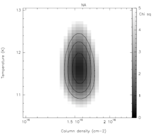
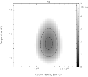
Figure 16: $\chi^{2}$ surface for the integrated intensity ratios at position NA.

Figure 17: $\chi^{2}$ surface for the integrated intensity ratios at position NB.

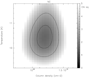
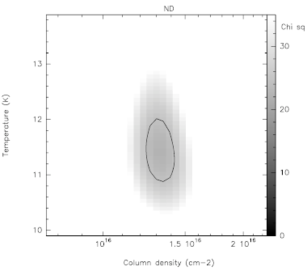
Figure 18: $\chi^{2}$ surface for the integrated intensity ratios at position NC.

Figure 19: $\chi^{2}$ surface for the integrated intensity ratios at position ND. Contour at 25.

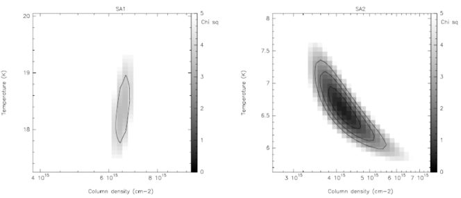
Figure 20: $\chi^{2}$ surfaces for the integrated intensity ratios at position SA: SA1 (LVC) on the left, and SA2 (HVC) on the right.

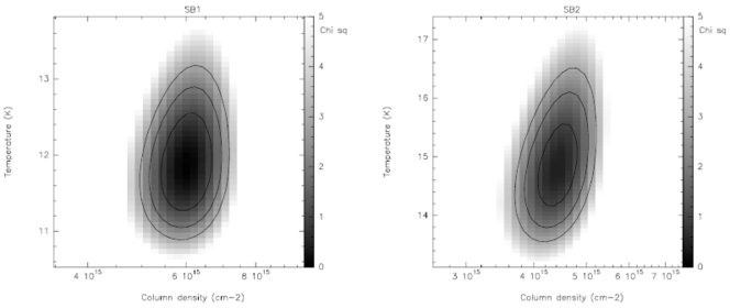
Figure 21: $\chi^{2}$ surface for the integrated intensity ratios at position SB: SB1 (LVC) on the left, and SB2 (HVC) on the right.

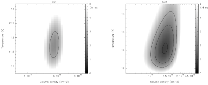
Figure 22: $\chi^{2}$ surface for the integrated intensity ratios at position SC: SC1 (LVC) on the left and SC2 (HVC) on the right.

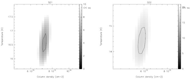
Figure 23: $\chi^{2}$ surface for the integrated intensity ratio at position SD: SD1 (LVC) on the left, and SD2 (HVC) on the right. Note the different colour scale for SC2. Contours are 6 for SD1 and 18 for SD2

Appendix B C¹⁸O intensities and abundances

Table 6 presents the best fit integrated intensities from the non-LTE (RADEX) modelling (§ A) , together with the observed values, and the implied C¹⁸O abundances.

Table 6: Modelled integrated intensities and resulting abundances.

		Observed			Best fit		H2	C18O	C18O
Position	I(1-0)	I(2-1)	I(3-2)	I(1-0)	I(2-1)	I(3-2)	column	column	fractional
		(K kms-1)			(K kms-1)		density	density	abundance
							($10^{23}$cm-2)	($10^{15}$cm-2)	($\times 10^{-8}$)
NA	9.15	10.65	6.94	9.23	10.42	7.28	1.60	15.4	9.6
NB	7.47	8.87	4.76	7.44	8.15	5.20	1.39	11.9	8.6
NC	8.14	10.35	4.90	8.13	9.29	5.57	1.00	11.9	12.0
ND	7.90	10.09	4.82	7.99	8.88	6.20	4.01	13.5	3.4
SA1	4.69	10.57	8.46	4.75	9.84	9.01	1.84	6.4	5.8
SA2	2.42	1.98	0.50	2.50	2.02	0.64		4.2
SB1	4.63	6.66	4.20	4.74	6.72	4.37	2.46	6.0	4.2
SB2	3.32	5.99	4.31	3.35	5.73	4.50		4.4
SC1	4.61	7.37	3.87	4.72	6.82	4.37	3.87	5.8	1.9
SC2	1.17	2.58	1.45	1.21	2.23	1.71		1.4
SD1	4.81	7.44	7.31	5.01	8.53	7.34	4.82	7.3	2.7
SD2	4.41	8.66	4.66	4.45	7.42	5.74		5.8

Positions of the NW sub-cluster are identified as starting with N, while the south positions start with S. For the positions in the SE, the labels 1 and 2 identify the lower (LVC) and higher velocity (HVC) components respectively. Where there are two velocity component lines, the C¹⁸O fractional abundance was calculated using the total column density of C¹⁸O, summing both components.

For positions ND, SB, SC and SD, the H₂ column densities derived from the dust and used to estimate the abundance of C¹⁸O were calculated using a dust temperature of 10K. Assuming a temperature of 15K for all 4 positions (ND, SB, SC and SD) would reduce the H₂ column densities by a factor of 2.1, representing an equivalent rise of the fractal abundance of C¹⁸O by the same amount.

The derived C¹⁸O fractional abundance (which is averaged along the line of sight) implies a depletion of C¹⁸O of between a factor of 1.4 (for NC) and 4.3 (for SC), with an average of 2.5 compared to the abundance of $1.7\times 10^{-7}$ in dark clouds (Frerking et al. 1982). Given that the ratio between C¹⁷O and C¹⁸O has shown these two species to be optically thin, with an intensity ratio of $\sim$3.5, a factor 2.5 depletion of C¹⁸O implies the same depletion factor for C¹⁷O.

References

- Blitz (1993) Blitz, L. 1993, in Protostars and Planets III, ed. E. H. Levy & J. I. Lunine, 125–161
- Cambrésy (1999) Cambrésy, L. 1999, A&A, 345, 965
- Curtis et al. (2009) Curtis, E. I., Richer, J. S., & Buckle, J. V. 2009, MNRAS, 1566
- Davis et al. (2000) Davis, C. J., Chrysostomou, A., Matthews, H. E., Jenness, T., & Ray, T. P. 2000, ApJ, 530, L115
- Davis et al. (1999) Davis, C. J., Matthews, H. E., Ray, T. P., Dent, W. R. F., & Richer, J. S. 1999, MNRAS, 309, 141
- Di Francesco et al. (2008) Di Francesco, J., Johnstone, D., Kirk, H., MacKenzie, T., & Ledwosinska, E. 2008, ApJS, 175, 277
- Eiroa et al. (1992) Eiroa, C., Torrelles, J. M., Gomez, J. F., et al. 1992, PASJ, 44, 155
- Enoch et al. (2007) Enoch, M. L., Glenn, J., Evans, II, N. J., et al. 2007, ApJ, 666, 982
- Frerking et al. (1982) Frerking, M. A., Langer, W. D., & Wilson, R. W. 1982, ApJ, 262, 590
- Fuller & Ladd (2002) Fuller, G. A. & Ladd, E. F. 2002, ApJ, 573, 699
- Fuller & Myers (1993) Fuller, G. A. & Myers, P. C. 1993, ApJ, 418, 273
- Graves et al. (2010) Graves, S. F., Richer, J. S., Buckle, J. V., et al. 2010, MNRAS, in press
- Harvey et al. (2007a) Harvey, P., Merín, B., Huard, T. L., et al. 2007a, ApJ, 663, 1149
- Harvey et al. (2007b) Harvey, P. M., Rebull, L. M., Brooke, T., et al. 2007b, ApJ, 663, 1139
- Hodapp (1999) Hodapp, K. W. 1999, AJ, 118, 1338
- Hogerheijde et al. (1999) Hogerheijde, M. R., van Dishoeck, E. F., Salverda, J. M., & Blake, G. A. 1999, ApJ, 513, 350
- Hurt & Barsony (1996) Hurt, R. L. & Barsony, M. 1996, ApJ, 460, L45+
- Hurt et al. (1996) Hurt, R. L., Barsony, M., & Wootten, A. 1996, ApJ, 456, 686
- Johnstone & Bally (2006) Johnstone, D. & Bally, J. 2006, ApJ, 653, 383
- Jørgensen et al. (2002) Jørgensen, J. K., Schöier, F. L., & van Dishoeck, E. F. 2002, A&A, 389, 908
- Kaas et al. (2004) Kaas, A. A., Olofsson, G., Bontemps, S., et al. 2004, Astronomy and Astrophysics, 421, 623
- Kitsionas & Whitworth (2007) Kitsionas, S. & Whitworth, A. P. 2007, MNRAS, 378, 507
- Lada & Lada (2003) Lada, C. J. & Lada, E. A. 2003, ARA&A, 41, 57
- Ladd et al. (1998) Ladd, E. F., Fuller, G. A., & Deane, J. R. 1998, ApJ, 495, 871
- Olmi & Testi (2002) Olmi, L. & Testi, L. 2002, A&A, 392, 1053
- Penzias (1980) Penzias, A. A. 1980, in IAU Symposium, Vol. 87, Interstellar Molecules, ed. B. H. Andrew, 397–402
- Peretto et al. (2006) Peretto, N., André, P., & Belloche, A. 2006, A&A, 445, 979
- Pineda et al. (2009) Pineda, J. E., Rosolowsky, E. W., & Goodman, A. A. 2009, ApJ, 699, L134
- Schoeier et al. (2005) Schoeier, F. L., van der Tak, F. F. S., van Dishoeck, E. F., & Black, J. H. 2005, VizieR Online Data Catalog, 343, 20369
- Straižys et al. (1996) Straižys, V., Černis, K., & Bartašiūte, S. 1996, Baltic Astronomy, 5, 125
- van der Tak et al. (2007) van der Tak, F. F. S., Black, J. H., Schöier, F. L., Jansen, D. J., & van Dishoeck, E. F. 2007, A&A, 468, 627
- van der Tak et al. (1999) van der Tak, F. F. S., van Dishoeck, E. F., Evans, II, N. J., Bakker, E. J., & Blake, G. A. 1999, ApJ, 522, 991
- Visser et al. (2009) Visser, R., van Dishoeck, E. F., Doty, S. D., & Dullemond, C. P. 2009, A&A, 495, 881
- Walsh et al. (2007) Walsh, A. J., Myers, P. C., Di Francesco, J., et al. 2007, ApJ, 655, 958
- Ward-Thompson et al. (2007) Ward-Thompson, D., Di Francesco, J., Hatchell, J., et al. 2007, PASP, 119, 855
- Williams et al. (1994) Williams, J. P., de Geus, E. J., & Blitz, L. 1994, ApJ, 428, 693
- Williams & Myers (1999) Williams, J. P. & Myers, P. C. 1999, ApJ, 518, L37
- Williams & Myers (2000) Williams, J. P. & Myers, P. C. 2000, ApJ, 537, 891