Slice sampling covariance hyperparameters
of latent Gaussian models

Abstract

The Gaussian process (GP) is a popular way to specify dependencies between random variables in a probabilistic model. In the Bayesian framework the covariance structure can be specified using unknown hyperparameters. Integrating over these hyperparameters considers different possible explanations for the data when making predictions. This integration is often performed using Markov chain Monte Carlo (MCMC) sampling. However, with non-Gaussian observations standard hyperparameter sampling approaches require careful tuning and may converge slowly. In this paper we present a slice sampling approach that requires little tuning while mixing well in both strong- and weak-data regimes.

1 Introduction

Many probabilistic models incorporate multivariate Gaussian distributions to explain dependencies between variables. Gaussian process (GP) models and generalized linear mixed models are common examples. For non-Gaussian observation models, inferring the parameters that specify the covariance structure can be difficult. Existing computational methods can be split into two complementary classes: deterministic approximations and Monte Carlo simulation. This work presents a method to make the sampling approach easier to apply.

In recent work Murray et al. [1] developed a slice sampling [2] variant, elliptical slice sampling, for updating strongly coupled a-priori Gaussian variates given non-Gaussian observations. Previously, Agarwal and Gelfand [3] demonstrated the utility of slice sampling for updating covariance parameters, conventionally called hyperparameters, with a Gaussian observation model, and questioned the possibility of slice sampling in more general settings. In this work we develop a new slice sampler for updating covariance hyperparameters. Our method uses a robust representation that should work well on a wide variety of problems, has very few technical requirements, little need for tuning and so should be easy to apply.

1.1 Latent Gaussian models

We consider generative models of data that depend on a vector of latent variables $\mathbf{f}$ that are Gaussian distributed with covariance $\Sigma_{\theta}$ set by unknown hyperparameters $\theta$. These models are common in the machine learning Gaussian process literature [e.g. 4] and throughout the statistical sciences. We use standard notation for a Gaussian distribution with mean $\mathbf{m}$ and covariance $\Sigma$,

$$\mathcal{N}(\mathbf{f};\mathbf{m},\Sigma)\equiv|2\pi\Sigma|^{-\nicefrac{{1}}{{2}}}\exp\kern-1.0pt\big{(}\vbox{\hbox{\scalebox{0.8}{$-{\textstyle\frac{1}{2}}(\mathbf{f}\!-\!\mathbf{m})^{\top}\Sigma^{-1}(\mathbf{f}\!-\!\mathbf{m})$}}}\big{)},$$ (1)

and use ${\mathbf{f}\sim\mathcal{N}(\mathbf{m},\Sigma)}$ to indicate that $\mathbf{f}$ is drawn from a distribution with the density in (1).

The generic form of the generative models we consider is summarized by

$$\begin{split}\text{covariance hyperparameters}&~{}~{}\theta\sim p_{h}\kern-1.0pt,\\ \text{latent variables}&~{}~{}\mathbf{f}\sim\mathcal{N}(0,\Sigma_{\theta}),\\ \text{and a conditional likelihood}&~{}~{}P(\mathrm{data}\kern 1.0pt|\kern 1.0pt\mathbf{f})=\mathcal{L}(\mathbf{f}).\end{split}$$

The methods discussed in this paper apply to covariances $\Sigma_{\theta}$ that are arbitrary positive definite functions parameterized by $\theta$. However, our experiments focus on the popular case where the covariance is associated with $N$ input vectors $\{\mathbf{x}_{n}\}_{n=1}^{N}$ through the squared-exponential kernel,

$$({\Sigma_{\theta}})_{ij}\kern-1.0pt=\kern-1.0ptk(\mathbf{x}_{i},\mathbf{x}_{j})\kern-1.0pt=\kern-1.0pt\sigma_{f}^{2}\exp\!\Big{(}\kern-2.0pt-\kern-1.0pt{\textstyle\frac{1}{2}}\kern-1.0pt\textstyle\sum_{d=1}^{D}\kern-3.0pt\frac{(x_{d,i}-x_{d,j})^{2}}{\ell_{d}^{2}}\kern-1.0pt\Big{)},$$ (2)

with hyperparameters $\theta\!=\!\{\sigma_{f}^{2},\{\ell_{d}\}\}$. Here $\sigma_{f}^{2}$ is the ‘signal variance’ controlling the overall scale of the latent variables $\mathbf{f}$. The $\ell_{d}$ give characteristic lengthscales for converting the distances between inputs into covariances between the corresponding latent values $\mathbf{f}$.

For non-Gaussian likelihoods we wish to sample from the joint posterior over unknowns,

$$P(\mathbf{f},\theta\kern 1.0pt|\kern 1.0pt\mathrm{data})=\textstyle\frac{1}{Z}\,\mathcal{L}(\mathbf{f})\,\mathcal{N}(\mathbf{f};0,\Sigma_{\theta})\,p_{h}\kern-1.0pt(\theta)\,.$$ (3)

We would like to avoid implementing new code or tuning algorithms for different covariances $\Sigma_{\theta}$ and conditional likelihood functions $\mathcal{L}(\mathbf{f})$.

2 Markov chain inference

A Markov chain transition operator $T(z^{\prime}\!\leftarrow\!z)$ defines a conditional distribution on a new position $z^{\prime}$ given an initial position $z$. The operator is said to leave a target distribution $\pi$ invariant if $\pi(z^{\prime})\!=\!\int T(z^{\prime}\!\leftarrow\!z)\,\pi(z)\;\mathrm{d}z$. A standard way to sample from the joint posterior (3) is to alternately simulate transition operators that leave its conditionals, $P(\mathbf{f}\kern 1.0pt|\kern 1.0pt\mathrm{data},\theta)$ and $P(\theta\kern 1.0pt|\kern 1.0pt\mathbf{f})$, invariant. Under fairly mild conditions the Markov chain will equilibrate towards the target distribution [e.g. 5].

Recent work has focused on transition operators for updating the latent variables $\mathbf{f}$ given data and a fixed covariance $\Sigma_{\theta}$ [6, 1]. Updates to the hyperparameters for fixed latent variables $\mathbf{f}$ need to leave the conditional posterior,

$$P(\theta\kern 1.0pt|\kern 1.0pt\mathbf{f})\propto\mathcal{N}(\mathbf{f};0,\Sigma_{\theta})\,p_{h}\kern-1.0pt(\theta),$$ (4)

invariant. The simplest algorithm for this is the Metropolis–Hastings operator, see Algorithm 1. Other possibilities include slice sampling [2] and Hamiltonian Monte Carlo [7, 8].

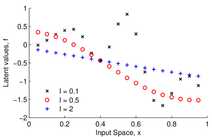
(a) Prior draws

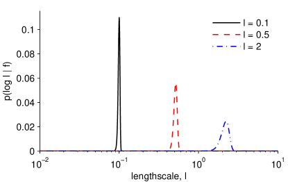
(b) Lengthscale given $\mathbf{f}$

Figure 1: LABEL:sub@fig:priordraws Shows draws from the prior over $\mathbf{f}$ using three different lengthscales in the squared exponential covariance (2). LABEL:sub@fig:postcondf Shows the posteriors over log-lengthscale for these three draws.

Alternately fixing the unknowns $\mathbf{f}$ and $\theta$ is appealing from an implementation standpoint. However, the resulting Markov chain can be very slow in exploring the joint posterior distribution. Figure 1a shows latent vector samples using squared-exponential covariances with different lengthscales. These samples are highly informative about the lengthscale hyperparameter that was used, especially for short lengthscales. The sharpness of $P(\theta\kern 1.0pt|\kern 1.0pt\mathbf{f})$, Figure 1b, dramatically limits the amount that any Markov chain can update the hyperparameters $\theta$ for fixed latent values $\mathbf{f}$.

2.1 Whitening the prior

Often the conditional likelihood is quite weak; this is why strong prior smoothing assumptions are often introduced in latent Gaussian models. In the extreme limit in which there is no data, i.e. $\mathcal{L}$ is constant, the target distribution is the prior model, $P(\mathbf{f},\theta)\!=\!\mathcal{N}(\mathbf{f};0,\Sigma_{\theta})\,p_{h}\kern-1.0pt(\theta)$. Sampling from the prior should be easy, but alternately fixing $\mathbf{f}$ and $\theta$ does not work well because they are strongly coupled. One strategy is to reparameterize the model so that the unknown variables are independent under the prior.

Independent random variables can be identified from a commonly-used generative procedure for the multivariate Gaussian distribution. A vector of independent normals, $\boldsymbol{\nu}$, is drawn independently of the hyperparameters and then deterministically transformed:

$$\boldsymbol{\nu}\sim\mathcal{N}(0,{\mathbb{I}}),\qquad\mathbf{f}=L_{\kern-1.0pt\Sigma_{\theta}}\boldsymbol{\nu},\qquad\text{where~{}}{L_{\kern-1.0pt\Sigma_{\theta}}^{\vphantom{\top}}L_{\kern-1.0pt\Sigma_{\theta}}^{\top}\!=\!\Sigma_{\theta}}.$$ (5)

Notation: Throughout this paper $L_{C}$ will be any user-chosen square root of covariance matrix $C$. While any matrix square root can be used, the lower-diagonal Cholesky decomposition is often the most convenient. We would reserve $C^{1/2}$ for the principal square root, because other square roots do not behave like powers: for example, $\mathrm{chol}(C)^{-1}\neq\mathrm{chol}(C^{-1})$.

We can choose to update the hyperparameters $\theta$ for fixed $\boldsymbol{\nu}$ instead of fixed $\mathbf{f}$. As the original latent variables $\mathbf{f}$ are deterministically linked to the hyperparameters $\theta$ in (5), these updates will actually change both $\theta$ and $\mathbf{f}$. The samples in Figure 1a resulted from using the same whitened variable $\boldsymbol{\nu}$ with different hyperparameters. They follow the same general trend, but vary over the lengthscales used to construct them.

The posterior over hyperparameters for fixed $\boldsymbol{\nu}$ is apparent by applying Bayes rule to the generative procedure in (5), or one can laboriously obtain it by changing variables in (3):

$$P(\theta\kern 1.0pt|\kern 1.0pt\boldsymbol{\nu},\mathrm{data})\propto P(\theta,\boldsymbol{\nu},\mathrm{data})=P(\theta,\mathbf{f}\!=\!L_{\kern-1.0pt\Sigma_{\theta}}\boldsymbol{\nu},\mathrm{data})\left|L_{\kern-1.0pt\Sigma_{\theta}}\right|\propto\dots\propto\mathcal{L}(\mathbf{f}(\theta,\boldsymbol{\nu}))\,p_{h}\kern-1.0pt(\theta).$$ (6)

Algorithm 2 is the Metropolis–Hastings operator for this distribution. The acceptance rule now depends on the latent variables through the conditional likelihood $\mathcal{L}(\mathbf{f})$ instead of the prior $\mathcal{N}(\mathbf{f};0,\Sigma_{\theta})$ and these variables are automatically updated to respect the prior. In the no-data limit, new hyperparameters proposed from the prior are always accepted.

Algorithm 1 M–H transition for fixed $\mathbf{f}$

1:Current $\mathbf{f}$ and hyperparameters $\theta$;
proposal dist. $q$; covariance function $\Sigma_{()}$.

2:Next hyperparameters

3:Propose: $\theta^{\prime}\sim q(\theta^{\prime}\,;\,\theta)$

4:Draw $u\sim\mathrm{Uniform}(0,1)$

5:if ${u<\frac{\mathcal{N}(\mathbf{f};0,\Sigma_{\theta^{\prime}})\,p_{h}\kern-1.0pt(\theta^{\prime})\,q(\theta\,;\,\theta^{\prime})}{\mathcal{N}(\mathbf{f};0,\Sigma_{\theta})\,p_{h}\kern-1.0pt(\theta)\,q(\theta^{\prime};\,\theta)}}$ 

6:     return $\theta^{\prime}$ $\triangleright$ Accept new state

7:else

8:     return $\theta$ $\triangleright$ Keep current state

Algorithm 2 M–H transition for fixed $\boldsymbol{\nu}$

1:Current state $\theta$, $\mathbf{f}$; proposal dist. $q$;
covariance function $\Sigma_{()}$; likelihood $\mathcal{L}()$.

2:Next $\theta$, $\mathbf{f}$

3:Solve for $\mathcal{N}(0,{\mathbb{I}})$ variate: $\boldsymbol{\nu}\!=\!L_{\kern-1.0pt\Sigma_{\theta}}^{-1}\mathbf{f}$

4:Propose $\theta^{\prime}\sim q(\theta^{\prime}\,;\,\theta)$

5:Compute implied values: $\mathbf{f}^{\prime}\!=\!L_{\kern-1.0pt\Sigma_{\theta^{\prime}}}\boldsymbol{\nu}$

6:Draw $u\sim\mathrm{Uniform}(0,1)$

7:if ${u<\frac{\mathcal{L}(\mathbf{f}^{\prime})\,p_{h}\kern-1.0pt(\theta^{\prime})\,q(\theta\,;\,\theta^{\prime})}{\mathcal{L}(\mathbf{f})\,p_{h}\kern-1.0pt(\theta)\,q(\theta^{\prime};\,\theta)}}$ 

8:     return $\theta^{\prime}$, $\mathbf{f}^{\prime}$ $\triangleright$ Accept new state

9:else

10:     return $\theta$, $\mathbf{f}$ $\triangleright$ Keep current state

3 Surrogate data model

Neither of the previous two algorithms are ideal for statistical applications, which is illustrated in Figure 2. Algorithm 2 is ideal in the “weak data” limit where the latent variables $\mathbf{f}$ are distributed according to the prior. In the example, the likelihoods are too restrictive for Algorithm 2’s proposal to be acceptable. In the “strong data” limit, where the latent variables $\mathbf{f}$ are fixed by the likelihood $\mathcal{L}$, Algorithm 1 would be ideal. However, the likelihood terms in the example are not so strong that the prior can be ignored.

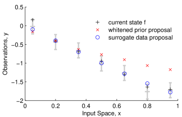
Figure 2: A regression problem with Gaussian observations illustrated by $2\sigma$ gray bars. The current state of the sampler has a short lengthscale hyperparameter ($\ell\!=\!0.3$); a longer lengthscale ($\ell\!=\!1.5$) is being proposed. The current latent variables do not lie on a straight enough line for the long lengthscale to be plausible. Whitening the prior (Section 2.1) updates the latent variables to a straighter line, but ignores the observations. A proposal using surrogate data (Section 3, with $S_{\theta}$ set to the observation noise) sets the latent variables to a draw that is plausible for the proposed lengthscale while being close to the current state.

For regression problems with Gaussian noise the latent variables can be marginalised out analytically, allowing hyperparameters to be accepted or rejected according to their marginal posterior $P(\theta\kern 1.0pt|\kern 1.0pt\mathrm{data})$. If latent variables are required they can be sampled directly from the conditional posterior $P(\mathbf{f}\kern 1.0pt|\kern 1.0pt\theta,\mathrm{data})$. To build a method that applies to non-Gaussian likelihoods, we create an auxiliary variable model that introduces surrogate Gaussian observations that will guide joint proposals of the hyperparameters and latent variables.

We augment the latent Gaussian model with auxiliary variables, $\mathbf{g}$, a noisy version of the true latent variables:

$$P(\mathbf{g}\kern 1.0pt|\kern 1.0pt\mathbf{f},\theta)=\mathcal{N}(\mathbf{g};\,\mathbf{f},S_{\theta}).$$ (7)

For now $S_{\theta}$ is an arbitrary free parameter that could be set by hand to either a fixed value or a value that depends on the current hyperparameters $\theta$. We will discuss how to automatically set the auxiliary noise covariance $S_{\theta}$ in Section 3.2.

The original model, $\mathbf{f}\sim\mathcal{N}(0,\Sigma_{\theta})$ and (7) define a joint auxiliary distribution $P(\mathbf{f},\mathbf{g}\kern 1.0pt|\kern 1.0pt\theta)$ given the hyperparameters. It is possible to sample from this distribution in the opposite order, by first drawing the auxiliary values from their marginal distribution

$$P(\mathbf{g}\kern 1.0pt|\kern 1.0pt\theta)=\mathcal{N}(\mathbf{g};\,0,\Sigma_{\theta}\!+\!S_{\theta}),$$ (8)

and then sampling the model’s latent values conditioned on the auxiliary values from

$$P(\mathbf{f}\kern 1.0pt|\kern 1.0pt\mathbf{g},\theta) =\mathcal{N}(\mathbf{f};\,\mathbf{m}_{\theta\kern-1.0pt,\mathbf{g}},R_{\theta}),\text{where some standard manipulations give:}$$

$$R_{\theta} =(\Sigma_{\theta}^{-1}\!+\!S_{\theta}^{-1})^{-1}=\Sigma_{\theta}\!-\!\Sigma_{\theta}(\Sigma_{\theta}\!+\!S_{\theta})^{-1}\Sigma_{\theta}=S_{\theta}\!-\!S_{\theta}(S_{\theta}\!+\!\Sigma_{\theta})^{-1}S_{\theta},$$

$$\mathbf{m}_{\theta\kern-1.0pt,\mathbf{g}} =\Sigma_{\theta}(\Sigma_{\theta}\!+\!S_{\theta})^{-1}\mathbf{g}=R_{\theta}^{\vphantom{-1}}S_{\theta}^{-1}\mathbf{g}.$$ (9)

That is, under the auxiliary model the latent variables of interest are drawn from their posterior given the surrogate data $\mathbf{g}$. Again we can describe the sampling process via a draw from a spherical Gaussian:

$$\boldsymbol{\eta}\sim\mathcal{N}(0,{\mathbb{I}}),\qquad\mathbf{f}=L_{\kern-1.0ptR_{\theta}}\boldsymbol{\eta}+\mathbf{m}_{\theta\kern-1.0pt,\mathbf{g}},\qquad\text{where~{}}{L_{\kern-1.0ptR_{\theta}}}^{\vphantom{\top}}L_{\kern-1.0ptR_{\theta}}^{\top}\!=\!R_{\theta}.$$ (10)

We then condition on the “whitened” variables $\boldsymbol{\eta}$ and the surrogate data $\mathbf{g}$ while updating the hyperparameters $\theta$. The implied latent variables $\mathbf{f}(\theta,\boldsymbol{\eta},\mathbf{g})$ will remain a plausible draw from the surrogate posterior for the current hyperparameters. This is illustrated in Figure 2.

We can leave the joint distribution (3) invariant by updating the following conditional distribution derived from the above generative model:

$$P(\theta\kern 1.0pt|\kern 1.0pt\boldsymbol{\eta},\mathbf{g},\mathrm{data})\propto P(\theta,\boldsymbol{\eta},\mathbf{g},\mathrm{data})\propto\mathcal{L}\big{(}\mathbf{f}(\theta,\boldsymbol{\eta},\mathbf{g})\big{)}\,\mathcal{N}(\mathbf{g};0,\Sigma_{\theta}\!+\!S_{\theta})\,p_{h}\kern-1.0pt(\theta).$$ (11)

The Metropolis–Hastings Algorithm 3 contains a ratio of these terms in the acceptance rule.

3.1 Slice sampling

The Metropolis–Hastings algorithms discussed so far have a proposal distribution $q(\theta^{\prime};\theta)$ that must be set and tuned. The efficiency of the algorithms depend crucially on careful choice of the scale $\sigma$ of the proposal distribution. Slice sampling [2] is a family of adaptive search procedures that are much more robust to the choice of scale parameter.

Algorithm 4 applies one possible slice sampling algorithm to a scalar hyperparameter $\theta$ in the surrogate data model of this section. It has a free parameter $\sigma$, the scale of the initial proposal distribution. However, careful tuning of this parameter is not required. If the initial scale is set to a large value, such as the width of the prior, then the width of the proposals will shrink to an acceptable range exponentially quickly. Stepping-out procedures [2] could be used to adapt initial scales that are too small. We assume that axis-aligned hyperparameter moves will be effective, although reparameterizations could improve performance [e.g. 9].

Algorithm 3 Surrogate data M–H

1:$\theta$, $\mathbf{f}$; prop. dist. $q$; model of Sec. 3.

2:Next $\theta$, $\mathbf{f}$

3:Draw surrogate data: $\mathbf{g}\sim\mathcal{N}(\mathbf{f},S_{\theta})$

4:Compute implied latent variates:
$\boldsymbol{\eta}\!=\!L_{\kern-1.0ptR_{\theta}}^{-1}(\mathbf{f}-\mathbf{m}_{\theta\kern-1.0pt,\mathbf{g}})$

5:Propose $\theta^{\prime}\sim q(\theta^{\prime}\,;\,\theta)$

6:Compute function $\mathbf{f}^{\prime}\!=\!L_{\kern-1.0ptR_{\theta^{\prime}}}\boldsymbol{\eta}+\boldsymbol{m}_{\theta^{\prime},\mathbf{g}}$

7:Draw $u\sim\mathrm{Uniform}(0,1)$

8:if ${u<\frac{\mathcal{L}(\mathbf{f}^{\prime})\,\mathcal{N}(\mathbf{g};0,\Sigma_{\theta^{\prime}}\!+\!S_{\theta^{\prime}})\,p_{h}\kern-1.0pt(\theta^{\prime})\,q(\theta\,;\,\theta^{\prime})}{\mathcal{L}(\mathbf{f})\,\mathcal{N}(\mathbf{g};0,\Sigma_{\theta}\!+\!S_{\theta})\,p_{h}\kern-1.0pt(\theta)\,q(\theta^{\prime}\,;\,\theta)}}$ 

9:     return $\theta^{\prime}$, $\mathbf{f}^{\prime}$ $\triangleright$ Accept new state

10:else

11:     return $\theta$, $\mathbf{f}$ $\triangleright$ Keep current state

Algorithm 4 Surrogate data slice sampling

1:$\theta$, $\mathbf{f}$; scale $\sigma$; model of Sec. 3.

2:Next $\mathbf{f}$, $\theta$

3:Draw surrogate data: $\mathbf{g}\sim\mathcal{N}(\mathbf{f},S_{\theta})$

4:Compute implied latent variates:
$\boldsymbol{\eta}\!=\!L_{\kern-1.0ptR_{\theta}}^{-1}(\mathbf{f}-\mathbf{m}_{\theta\kern-1.0pt,\mathbf{g}})$

5:Randomly center a bracket:$v\sim\mathrm{Uniform}(0,\sigma),\;\;\theta_{\sf{min}}\!=\!\theta\!-\!v,\;\;\theta_{\sf{max}}\!=\!\theta_{\sf{min}}\!+\!\sigma$

6:Draw $u\sim\mathrm{Uniform}(0,1)$

7:Determine threshold:
$y=u\,\mathcal{L}(\mathbf{f})\,\mathcal{N}(\mathbf{g};0,\Sigma_{\theta}\!+\!S_{\theta})\,p_{h}\kern-1.0pt(\theta)$

8:Draw proposal: $\theta^{\prime}\sim\mathrm{Uniform}(\theta_{\sf{min}},\theta_{\sf{max}})$

9:Compute function $\mathbf{f}^{\prime}\!=\!L_{\kern-1.0ptR_{\theta^{\prime}}}\boldsymbol{\eta}+\boldsymbol{m}_{\theta^{\prime},\mathbf{g}}$

10:if $\mathcal{L}(\mathbf{f}^{\prime})\,\mathcal{N}(\mathbf{g};0,\Sigma_{\theta^{\prime}}\!+\!S_{\theta^{\prime}})\,p_{h}\kern-1.0pt(\theta^{\prime})>y$ 

11:     return $\mathbf{f}^{\prime}$, $\theta^{\prime}$

12:else if $\theta^{\prime}<\theta$ 

13:     Shrink bracket minimum: $\theta_{\sf{min}}=\theta^{\prime}$

14:else

15:     Shrink bracket maximum: $\theta_{\sf{max}}=\theta^{\prime}$

16:goto 8

3.2 The auxiliary noise covariance $S_{\theta}$

The surrogate data $\mathbf{g}$ and noise covariance $S_{\theta}$ define a pseudo-posterior distribution that softly specifies a plausible region within which the latent variables $\mathbf{f}$ are updated. The noise covariance determines the size of this region. The first two baseline algorithms of Section 2 result from limiting cases of $S_{\theta}\!=\!\alpha{\mathbb{I}}$: 1) if $\alpha\!=\!0$ the surrogate data and the current latent variables are equal and the acceptance ratio reduces to that of Algorithm 1. 2) as $\alpha\!\rightarrow\!\infty$ the observations are uninformative about the current state and the pseudo-posterior tends to the prior. In the limit, the acceptance ratio reduces to that of Algorithm 2. One could choose $\alpha$ based on preliminary runs, but such tuning would be burdensome.

For likelihood terms that factorize, $\mathcal{L}(\mathbf{f})\!=\!\prod_{i}\mathcal{L}_{i}(f_{i})$, we can measure how much the likelihood restricts each variable individually:

$$P(f_{i}\kern 1.0pt|\kern 1.0pt\mathcal{L}_{i},\theta)\propto\mathcal{L}_{i}(f_{i})\;\mathcal{N}(f_{i};0,(\Sigma_{\theta})_{ii}).$$ (12)

A Gaussian can be fitted by moment matching or a Laplace approximation (matching second derivatives at the mode). Such fits, or close approximations, are often possible analytically and can always be performed numerically as the distribution is only one-dimensional. Given a Gaussian fit to the site-posterior (12) with variance $v_{i}$, we can set the auxiliary noise to a level that would result in the same posterior variance at that site alone: ${(S_{\theta})_{ii}\!=\!(v_{i}^{-1}\!-\!{(\Sigma_{\theta})_{ii}}^{-1})^{-1}}$. (Any negative $(S_{\theta})_{ii}$ must be thresholded.) The moment matching procedure is a grossly simplified first step of “assumed density filtering” or “expectation propagation” [10], which are too expensive for our use in the inner-loop of a Markov chain.

4 Related work

We have discussed samplers that jointly update strongly-coupled latent variables and hyperparameters. The hyperparameters can move further in joint moves than their narrow conditional posteriors (e.g., Figure 1b) would allow. A generic way of jointly sampling real-valued variables is Hamiltonian/Hybrid Monte Carlo (HMC) [7, 8]. However, this method is cumbersome to implement and tune, and using HMC to jointly update latent variables and hyperparameters in hierarchical models does not itself seem to improve sampling [11].

Christensen et al. [9] have also proposed a robust representation for sampling in latent Gaussian models. They use an approximation to the target posterior distribution to construct a reparameterization where the unknown variables are close to independent. The approximation replaces the likelihood with a Gaussian form proportional to $\mathcal{N}(\mathbf{f};\hat{\mathbf{f}},\Lambda(\hat{\mathbf{f}}))$:

$$\textstyle\hat{\mathbf{f}}=\operatorname*{argmax}_{\mathbf{f}}\mathcal{L}(\mathbf{f}),\qquad\Lambda_{ij}(\hat{\mathbf{f}})=\left.\frac{\partial^{2}\log\mathcal{L}(\mathbf{f})}{\partial f_{i}\,\partial f_{j}}\right|_{\hat{\mathbf{f}}},$$ (13)

where $\Lambda$ is often diagonal, or it was suggested one would only take the diagonal part. This Taylor approximation looks like a Laplace approximation, except that the likelihood function is not a probability density in $\mathbf{f}$. This likelihood fit results in an approximate Gaussian posterior $\mathcal{N}(\mathbf{f};\mathbf{m}_{\theta\kern-1.0pt,\mathbf{g}=\hat{\mathbf{f}}},R_{\theta})$ as found in (9), with noise $S_{\theta}\!=\!\Lambda(\hat{\mathbf{f}})^{-1}$ and data $\mathbf{g}\!=\!\hat{\mathbf{f}}$.

Thinking of the current latent variables as a draw from this approximate posterior, ${\boldsymbol{\omega}\!\sim\!\mathcal{N}(0,{\mathbb{I}})},\hskip 4.30554pt\mathbf{f}\!=\!L_{\kern-1.0ptR_{\theta}}\boldsymbol{\omega}\!+\!\mathbf{m}_{\theta\kern-1.0pt,\hat{\mathbf{f}}}$, suggests using the reparameterization ${\boldsymbol{\omega}=L_{\kern-1.0ptR_{\theta}}^{-1}(\mathbf{f}-\mathbf{m}_{\theta\kern-1.0pt,\hat{\mathbf{f}}})}$. We can then fix the new variables and update the hyperparameters under

$$P(\theta\kern 1.0pt|\kern 1.0pt\boldsymbol{\omega},\mathrm{data})\propto\mathcal{L}(\mathbf{f}(\boldsymbol{\omega},\theta))\,\mathcal{N}(\mathbf{f}(\boldsymbol{\omega},\theta);0,\Sigma_{\theta})\,p_{h}\kern-1.0pt(\theta)\left|L_{\kern-1.0ptR_{\theta}}\right|.$$ (14)

When the likelihood is Gaussian, the reparameterized variables $\boldsymbol{\omega}$ are independent of each other and the hyperparameters. The hope is that approximating non-Gaussian likelihoods will result in nearly-independent parameterizations on which Markov chains will mix rapidly.

Taylor expanding some common log-likelihoods around the maximum is not well defined, for example approximating probit or logistic likelihoods for binary classification, or Poisson observations with zero counts. These Taylor expansions could be seen as giving flat or undefined Gaussian approximations that do not reweight the prior. When all of the likelihood terms are flat the reparameterization approach reduces to that of Section 2.1. The alternative $S_{\theta}$ auxiliary covariances that we have proposed could be used instead.

The surrogate data samplers of Section 3 can also be viewed as using reparameterizations, by treating $\boldsymbol{\eta}\!=\!L_{\kern-1.0ptR_{\theta}}^{-1}(\mathbf{f}-\mathbf{m}_{\theta\kern-1.0pt,\mathbf{g}})$ as an arbitrary random reparameterization for making proposals. A proposal density $q(\boldsymbol{\eta}^{\prime},\theta^{\prime};\boldsymbol{\eta},\theta)$ in the reparameterized space must be multiplied by the Jacobian $|L_{\kern-1.0ptR_{\theta^{\prime}}}^{-1}|$ to give a proposal density in the original parameterization. The probability of proposing the reparameterization must also be included in the Metropolis–Hastings acceptance probability:

$$\textstyle\min\left(1,\;\frac{P(\theta^{\prime},\mathbf{f}^{\prime}\kern 1.0pt|\kern 1.0pt\mathrm{data})\cdot P(\mathbf{g}\kern 1.0pt|\kern 1.0pt\mathbf{f}^{\prime},S_{\theta^{\prime}})\cdot q(\theta;\theta^{\prime})\,|L_{\kern-1.0ptR_{\theta}}^{-1}|}{P(\theta,\mathbf{f}\kern 1.0pt|\kern 1.0pt\mathrm{data})\cdot P(\mathbf{g}\kern 1.0pt|\kern 1.0pt\mathbf{f},S_{\theta})\cdot q(\theta^{\prime};\theta)\,|L_{\kern-1.0ptR_{\theta^{\prime}}}^{-1}|}\right).$$ (15)

A few lines of linear algebra confirms that, as it must do, the same acceptance ratio results as before. Alternatively, substituting (3) into (15) shows that the acceptance probability is very similar to that obtained by applying Metropolis–Hastings to (14) as proposed by Christensen et al. [9]. The differences are that the new latent variables $\mathbf{f}^{\prime}$ are computed using different pseudo-posterior means and the surrogate data method has an extra term for the random, rather than fixed, choice of reparameterization.

The surrogate data sampler is easier to implement than the previous reparameterization work because the surrogate posterior is centred around the current latent variables. This means that 1) no point estimate, such as the maximum likelihood $\hat{\mathbf{f}}$, is required. 2) picking the noise covariance $S_{\theta}$ poorly may still produce a workable method, whereas a fixed reparameterized can work badly if the true posterior distribution is in the tails of the Gaussian approximation. Christensen et al. [9] pointed out that centering the approximate Gaussian likelihood in their reparameterization around the current state is tempting, but that computing the Jacobian of the transformation is then intractable. By construction, the surrogate data model centers the reparameterization near to the current state.

5 Experiments

We empirically compare the performance of the various approaches to GP hyperparameter sampling on four data sets: one regression, one classification, and two Cox process inference problems. Further details are in the rest of this section, with full code as supplementary material. The results are summarized in Figure 3 followed by a discussion section.

In each of the experimental configurations, we ran ten independent chains with different random seeds, burning in for 1000 iterations and sampling for 5000 iterations. We quantify the mixing of the chain by estimating the effective number of samples of the complete data likelihood trace using R-CODA [12], and compare that with three cost metrics: the number of hyperparameter settings considered (each requiring a small number of covariance decompositions with $O(n^{3})$ time complexity), the number of likelihood evaluations, and the total elapsed time on a single core of an Intel Xeon 3GHz CPU.

The experiments are designed to test the mixing of hyperparameters $\theta$ while sampling from the joint posterior (3). All of the discussed approaches except Algorithm 1 update the latent variables $\mathbf{f}$ as a side-effect. However, further transition operators for the latent variables for fixed hyperparameters are required. In Algorithm 2 the “whitened” variables $\boldsymbol{\nu}$ remain fixed; the latent variables and hyperparameters are constrained to satisfy $\mathbf{f}\!=\!L_{\kern-1.0pt\Sigma_{\theta}}\boldsymbol{\nu}$. The surrogate data samplers are ergodic: the full joint posterior distribution will eventually be explored. However, each update changes the hyperparameters and requires expensive computations involving covariances. After computing the covariances for one set of hyperparameters, it makes sense to apply several cheap updates to the latent variables. For every method we applied ten updates of elliptical slice sampling [1] to the latent variables $\mathbf{f}$ between each hyperparameter update. One could also consider applying elliptical slice sampling to a reparameterized representation, for simplicity of comparison we do not. Independently of our work Titsias [13] has used surrogate data like reparameterizations to update latent variables for fixed hyperparameters.

Methods

We implemented six methods for updating Gaussian covariance hyperparameters. Each method used the same slice sampler, as in Algorithm 4, applied to the following model representations. fixed: fixing the latent function $\mathbf{f}$ [14]. prior-white: whitening with the prior. surr-site: using surrogate data with the noise level set to match the site posterior (12). We used Laplace approximations for the Poisson likelihood. For classification problems we used moment matching, because Laplace approximations do not work well [15]. surr-taylor: using surrogate data with noise variance set via Taylor expansion of the log-likelihood (13). Infinite variances were truncated to a large value. post-taylor and post-site: as for the surr- methods but a fixed reparameterization based on a posterior approximation (14).

Binary Classification (Ionosphere)

We evaluated four different methods for performing binary GP classification: fixed, prior-white, surr-site and post-site. We applied these methods to the Ionosphere dataset [16], using 200 training data and 34 dimensions. We used a logistic likelihood with zero-mean prior, inferring lengthscales as well as signal variance. The -taylor methods reduce to other methods or don’t apply because the maximum of the log-likelihood is at plus or minus infinity.

Gaussian Regression (Synthetic)

When the observations have Gaussian noise the post-taylor reparameterization of Christensen et al. [9] makes the hyperparameters and latent variables exactly independent. The random centering of the surrogate data model will be less effective. We used a Gaussian regression problem to assess how much worse the surrogate data method is compared to an ideal reparameterization. The synthetic data set had 200 input points in 10-D drawn uniformly within a unit hypercube. The GP had zero mean, unit signal variance and its ten lengthscales in (2) drawn from $\mathrm{Uniform}(0,\surd{10})$. Observation noise had variance 0.09. We applied the fixed, prior-white, surr-site/surr-taylor, and post-site/post-taylor methods. For Gaussian likelihoods the -site and -taylor methods coincide: the auxiliary noise matches the observation noise ($S_{\theta}=0.09\,{\mathbb{I}}$).

Cox process inference

We tested all six methods on an inhomogeneous Poisson process with a Gaussian process prior for the log-rate. We sampled the hyperparameters in (2) and a mean offset to the log-rate. The model was applied to two point process datasets: 1) a record of mining disasters [17] with 191 events in 112 bins of 365 days. 2) 195 redwood tree locations in a region scaled to the unit square [18] split into $25\!\times\!25\!=\!625$ bins. The results for the mining problem were initially highly variable. As the mining experiments were also the quickest we re-ran each chain for 20,000 iterations.

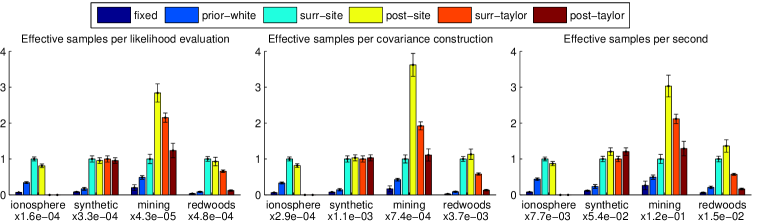
Figure 3: The results of experimental comparisons of six MCMC methods for GP hyperparameter inference on four data sets. Each figure shows four groups of bars (one for each experiment) and the vertical axis shows the effective number of samples of the complete data likelihood per unit cost. The costs are per likelihood evaluation (left), per covariance construction (center), and per second (right). Means and standard errors for 10 runs are shown. Each group of bars has been rescaled for readability: the number beneath each group gives the effective samples for the surr-site method, which always has bars of height 1. Bars are missing where methods are inapplicable (see text).

6 Discussion

On the Ionosphere classification problem both of the -site methods worked much better than the two baselines. We slightly prefer surr-site as it involves less problem-specific derivations than post-site.

On the synthetic test the post- and surr- methods perform very similarly. We had expected the existing post- method to have an advantage of perhaps up to 2–3$\times$, but that was not realized on this particular dataset. The post- methods had a slight time advantage, but this is down to implementation details and is not notable.

On the mining problem the Poisson likelihoods are often close to Gaussian, so the existing post-taylor approximation works well, as do all of our new proposed methods. The Gaussian approximations to the Poisson likelihood fit most poorly to sites with zero counts. The redwood dataset discretizes two-dimensional space, leading to a large number of bins. The majority of these bins have zero counts, many more than the mining dataset. Taylor expanding the likelihood gives no likelihood contribution for bins with zero counts, so it is unsurprising that post-taylor performs similarly to prior-white. While surr-taylor works better, the best results here come from using approximations to the site-posterior (12). For unreasonably fine discretizations the results can be different again: the site- reparameterizations do not always work well.

Our empirical investigation used slice sampling because it is easy to implement and use. However, all of the representations we discuss could be combined with any other MCMC method, such as [19] recently used for Cox processes. The new surrogate data and post-site representations offer state-of-the-art performance and are the first such advanced methods to be applicable to Gaussian process classification.

An important message from our results is that fixing the latent variables and updating hyperparameters according to the conditional posterior — as commonly used by GP practitioners — can work exceedingly poorly. Even the simple reparameterization of “whitening the prior” discussed in Section 2.1 works much better on problems where smoothness is important in the posterior. Even if site approximations are difficult and the more advanced methods presented are inapplicable, the simple whitening reparameterization should be given serious consideration when performing MCMC inference of hyperparameters.

Acknowledgements

We thank an anonymous reviewer for useful comments. This work was supported in part by the IST Programme of the European Community, under the PASCAL2 Network of Excellence, IST-2007-216886. This publication only reflects the authors’ views. RPA is a junior fellow of the Canadian Institute for Advanced Research.

References

- Murray et al. [2010] Iain Murray, Ryan Prescott Adams, and David J.C. MacKay. Elliptical slice sampling. Journal of Machine Learning Research: W&CP, 9:541–548, 2010. Proceedings of the 13th International Conference on Artificial Intelligence and Statistics (AISTATS).
- Neal [2003] Radford M. Neal. Slice sampling. Annals of Statistics, 31(3):705–767, 2003.
- Agarwal and Gelfand [2005] Deepak K. Agarwal and Alan E. Gelfand. Slice sampling for simulation based fitting of spatial data models. Statistics and Computing, 15(1):61–69, 2005.
- Rasmussen and Williams [2006] Carl Edward Rasmussen and Christopher K. I. Williams. Gaussian Processes for machine learning. MIT Press, 2006.
- Tierney [1994] Luke Tierney. Markov chains for exploring posterior distributions. The Annals of Statistics, 22(4):1701–1728, 1994.
- Titsias et al. [2009] Michalis Titsias, Neil D Lawrence, and Magnus Rattray. Efficient sampling for Gaussian process inference using control variables. In Advances in Neural Information Processing Systems 21, pages 1681–1688. MIT Press, 2009.
- Duane et al. [1987] Simon Duane, A. D. Kennedy, Brian J. Pendleton, and Duncan Roweth. Hybrid Monte Carlo. Physics Letters B, 195(2):216–222, September 1987.
- [8] Radford M. Neal. MCMC using Hamiltonian dynamics. To appear in the Handbook of Markov Chain Monte Carlo, Chapman & Hall / CRC Press, 2011. http://www.cs.toronto.edu/~radford/ftp/ham-mcmc.pdf.
- Christensen et al. [2006] Ole F. Christensen, Gareth O. Roberts, and Martin Skãld. Robust Markov chain Monte Carlo methods for spatial generalized linear mixed models. Journal of Computational and Graphical Statistics, 15(1):1–17, 2006.
- Minka [2001] Thomas Minka. Expectation propagation for approximate Bayesian inference. In Proceedings of the 17th Annual Conference on Uncertainty in Artificial Intelligence (UAI), pages 362–369, 2001. Corrected version available from http://research.microsoft.com/~minka/papers/ep/.
- Choo [2000] Kiam Choo. Learning hyperparameters for neural network models using Hamiltonian dynamics. Master’s thesis, Department of Computer Science, University of Toronto, 2000. Available from http://www.cs.toronto.edu/~radford/ftp/kiam-thesis.ps.
- Cowles et al. [2006] Mary Kathryn Cowles, Nicky Best, Karen Vines, and Martyn Plummer. R-CODA 0.10-5, 2006. http://www-fis.iarc.fr/coda/.
- Titsias [2010] Michalis Titsias. Auxiliary sampling using imaginary data, 2010. Unpublished.
- Neal [1999] Radford M. Neal. Regression and classification using Gaussian process priors. In J. M. Bernardo et al., editors, Bayesian Statistics 6, pages 475–501. OU Press, 1999.
- Kuss and Rasmussen [2005] Malte Kuss and Carl Edward Rasmussen. Assessing approximate inference for binary Gaussian process classification. Journal of Machine Learning Research, 6:1679–1704, 2005.
- Sigillito et al. [1989] V. G. Sigillito, S. P. Wing, L. V. Hutton, and K. B. Baker. Classification of radar returns from the ionosphere using neural networks. Johns Hopkins APL Technical Digest, 10:262–266, 1989.
- Jarrett [1979] R. G. Jarrett. A note on the intervals between coal-mining disasters. Biometrika, 66(1):191–193, 1979.
- Ripley [1977] Brian D. Ripley. Modelling spatial patterns. Journal of the Royal Statistical Society, Series B, 39:172–212, 1977.
- Girolami and Calderhead [2011] Mark Girolami and Ben Calderhead. Riemann manifold Langevin and Hamiltonian Monte Carlo methods. Journal of the Royal Statistical Society. Series B (Methodological), 2011. To appear.