PINGSoft: an IDL visualisation and manipulation tool
for Integral Field Spectroscopic data

Abstract

In this article we introduce PINGSoft, a set of IDL routines designed to visualise and manipulate, in an interactive and friendly way, Integral Field Spectroscopic data. The package is optimised for large databases and a fast visualisation rendering. Here we describe its major characteristics and requirements, providing examples and describing its capabilities. The PINGSoft package is freely available at: http://www.ast.cam.ac.uk/research/pings

1 Introduction

The data reduction, manipulation and visualisation of Integral Field Spectroscopy (IFS) observations possess an intrinsic complexity given the nature of the data and the vast amount of information recorded even in a single observation. In spite of the obvious advantages of this technique in tackling known scientific problems, in opening up new lines of research, and the increasing number of instruments available to astronomers, 2-dimensional (2D) spectroscopy is a technique that is relatively little used.

Nowadays only few groups around the world are capable of reducing and analysing, in a systematic and homogeneous way, the huge volume of data generated by IFS observations, and these groups tend to be involved with a particular instrument, implying that most 2D data reduction, visualization and analysis packages are orientated towards and limited to a single instrument, so that experience with one instrument does not necessarily guarantee the ability to work on another.

The data processing of IFS observations requires several steps before any science can be extracted, and some of them are particular for specific science cases. They include the (complex) data reduction, mapping, source extraction, continuum fitting, emission/absorption line fitting, deconvolution, cross-correlation, etc. Most of these operations are not independent tasks, and visual/spatial checking of the cube at every step is essential for a correct data treatment and eventual scientific interpretation. On this regard, exploring, visualising and manipulating IFS reduced data by standard means still represents a challenge in the 2D spectroscopy community, fact that perhaps has discouraged part of the community into getting involved to this field.

There have been important efforts towards a standardisation of IFS visualisation and manipulation tools, one is represented by the Euro3D Research Training Network (Walsh and Roth, 2002), who developed the E3D visualization tool (Sánchez, 2004), a package which allows the user to view an 2D image at any wavelength slice, to explore the spectra at any spaxel, and to perform simple analyses, being capable of handling several data formats. Its main limitation resides in the multiple library dependencies during installation, specially important for non-native linux platforms. QFitsView by Thomas Ott, is a generic FITS viewer program capable of handling IFS data and performing basic analysis operations on practically any OS flavour. However on most cases, the final reduced cubes need to be reformatted in order to use this tool.

Other major astronomical packages include visualisation and manipulation tools for IFS data as part of their releases, examples are the GAIA and DATACUBE packages, as part of the Starlink project, the wavextract IRAF task (by Jeremy Walsh) and some expected 3D tools in the upgrade of the Groningen Image Processing System, GIPSY (van der Hulst et al., 1992). The recently launched p3d software for IFS data reduction (Sandin et al., 2010) also integrates some level of visualisation, but it is restricted to the reduction pipeline. All these tools allow a quick-look and basic manipulation of IFS observations, but depend to a certain extent on their major software packages, and in some cases, on compilation libraries and data formats. Furthermore, they are restricted to a graphical user interface (GUI), without a command-line based option, which might be a restriction while handling large IFS databases.

In order to overcome some of these limitations, the PINGSoft package was envisaged, i.e. a set of tools especially designed to visualise and manipulate, in an interactive and friendly way, IFS data regardless of the original instrument and spaxel size/shape, able to run on practically any computer platform and with minimal library requirements. In this article, the PINGSoft package is presented, including a general description of the program, installation requirements, examples of its performance with real data and a summary of all routines included within the distribution, in the hope that the community will find it useful, and in a way to contribute with the proliferation of IFS-based astronomical research.

2 The PINGSoft package

The PINGS software, or PINGSoft, was originally developed during the PPAK IFS Nearby Galaxies Survey, or PINGS project (Rosales-Ortega et al., 2010), which used the PMAS (Roth et al., 2005) Integral Field Unit (IFU) in the PPAK mode (Verheijen et al., 2004; Kelz et al., 2006; Kelz and Roth, 2006) at the Centro Astronómico Hispano Alemán (CAHA) at Calar Alto, Spain. Given the large size of the 2D spectroscopic mosaics observed by PINGS, these routines were conceived to handle a large amount of data, therefore their implementation for equal or smaller fields of view and/or with similar instrumental setups is straightforward.

PINGSoft is written in the IDL programming language and consists of a set of individual routines called as command lines with a specific syntax in an IDL running terminal. The main drawback of the IDL environment is its commercial character. However, nowadays practically any astronomical centre around the world has a running institutional license of IDL available for its community, making possible to install very easily any IDL-based software, without compilation/library dependencies and/or platform issues.

The PINGSoft routines should be seen as the starting point to visualise and manipulate the (usually) large data formats produced by any IFU observation. More sophisticated visualisation and analysis would require tailored-built codes for the specific instrument and scientific case. However, given that the PINGSoft codes are not in the form of pre-compiled binaries and the source is completely open, the user can extract and modify any of the routines for more specific and personalised tasks, which is another advantage compared to other pre-compiled visualisation software.

In terms of data formats, practically any IFS data can be adapted to work with PINGSoft, regardless of the original data format (e.g. 3D cubes, RSS, FITS tables, etc.), and the size/shape of the spaxel. Given that these routines were developed for the PPAK instrument, they are perfectly suited for they immediate implementation to the CALIFA data.

The public version of PINGSoft includes the basic tools to visualise spatially and spectrally the IFS data, to extract regions of interest by hand or within a given geometric aperture, to integrate the spectra within a given region, to read, edit and write IFS FITS files, and to perform simple analyses to the IFS data. Additionally, some miscellaneous codes useful for generic tasks performed in astronomy and spectroscopy are also included. For more sophisticated visualisation/analyses the updated versions of the E3D and R3D software (Sánchez, 2004, 2006) are recommended, which include several routines for a detailed semi-automated spectroscopic analysis (SSP continuum fitting, emission line fitting, etc.).

3 Installation requirements

All the installation requirements and instructions are explained in detailed in the PINGSoft documentation found at the project webpage. Here we just summarise the main requirements and installations steps to give the reader an idea of the complexity in the installation of PINGSoft.

In order to run properly, PINGSoft should be installed in a UNIX, Linux, Mac or Windows computer via a terminal window running any IDL version greater than 6.0. The user should download the TAR file containing the PINGSoft library (i.e. pingsoft.tar.gz) from the project webpage, then extract it into a folder of his preference. This will create a directory named pingsoft/, with all the codes of the distribution and additional subdirectories. In order to work properly, PINGSoft requires the entire content of both the NASA IDL Astronomy User’s Library and the set of routines created by David W. Fanning, known as the Coyote Library. As these are very common IDL routines, they are probably already installed as part of the IDL library of the user’s institute. Otherwise, a personal copy can be downloaded from http://idlastro.gsfc.nasa.gov and http://www.dfanning.com/documents/programs.html respectively; both libraries must be extracted and installed in the same way as PINGSoft. Finally, the pingsoft/ directory (as well as any other new library) and a PINGSOFT_PATH variable should be defined in the user’s system, e.g. at the startup script that controls the shell of the OS system.

This is everything that the user needs to install the package, to check if the installation was done correctly, open a new terminal and type:

% echo $PINGSOFT_PATH

which should print something like: /path_to_your_IDL_directory/pingsoft

Then, in an IDL running terminal:

IDL> check_pingsoft
% Compiled module: CHECK_PINGSOFT.
% Compiled module: PINGSOFT_DISPLAY.

 Checking display...

 Checking paths...

 Checking files...

 PINGSoft installed successfully...!

4 The RSS data format

PINGSoft works with the Row Stacked Spectra or RSS format (Sánchez, 2004, 2006), plus a corresponding position table in ASCII format. A RSS file consists in a 2D FITS image in which the $X$-axis corresponds to the dispersion axis, and the other one corresponds to a given spatial ordering of the spectra determined by the position table, i.e. the $N$-row in the $Y$-axis corresponds to the spectrum at the position $(X_{N},\,Y_{N})\equiv(\Delta{\rm RA}_{N},\,\Delta{\rm Dec}_{N})$ from a $(0,\,0)$ reference point (in arcseconds), which is the $N$ entry of the ASCII file position table. The number of rows on the RSS FITS file is equal to the total number of spectra of the IFS data, i.e. the spectra are stacked one on top of each other in the $Y$-axis. This is the standard output format for reduced PMAS/PPAK data, and for the PINGS and CALIFA projects.

For instruments in which the standard output is a 3D spectral cube, individual spectra can be extracted at any spatial position and stored in a RSS file. The spatial location of the spectra can be then recorded in a ASCII file to create the position table. This technique has been tested successfully with data obtained with the VIMOS instrument (Fevre et al., 1998). The cube2rss.pro routine included in PINGSoft can easily convert a 3D cube into a RSS file.

The format of the input position table should be the following:

C       1.34       1.34      1
1     -13.936      0.000     1
2      15.686      3.019     1
3       0.000     12.071     1
4     -13.936     12.077     1
5      13.935     12.077     1
6     -10.452      6.038     1
...

where the first line determines the size and shape of the spaxel (see below), and the following entries correspond to: ID_# X_offset Y_offset flag, where ID_# is the spectrum number identification (integer value) and flag might be any numerical value (used sometimes for internal quality control). The size and shape of the spaxels is determined by the first two entries of the first line of the position table, the first character should be either a C or S, which corresponds to a circular (e.g. fibre, PPAK) or square (e.g. PMAS, VIMOS) spaxel, and the second entry should be a floating number corresponding to the radius or side length respectively, e.g.:

    C  1.34    (’C’ircular spaxel, with a radius 1.34 arcsec, e.g. PPAK)

    S  0.67    (’S’quare spaxel, with sides of length 0.67 arcsec, e.g. VIMOS)

the $PINGSOFT_PATH/pos_tables directory contains more position table examples.

In addition to the format restrictions mentioned above, the RSS file should be wavelength calibrated and the spectral information should be included in the FITS header, namely the CRPIX1, CRVAL1 and CDELT1 values. If the IFS data to analyse is in the RSS format with corresponding position tables, then PINGSoft should work smoothly and the visualisation/manipulation should be straightforward (e.g. CALIFA data).

5 PINGSoft by examples

All the PINGSoft routines are called via command lines in a terminal running IDL. The syntax of any program can be obtained by entering the name of the procedure without any other parameter. The routines are also documented within the .pro files, where an explanation, syntax and examples of the routines are included as comments at the beginning of the file.

The potential of the software can be illustrated by introducing the prototype procedure from which the rest of the main routines were based. This code is called view_rss.pro, which displays interactively a visualisation of any RSS file, including its spatial and spectral information. The PINGSoft distribution includes some RSS example files in the directory $PINGSOFT_PATH/examples/, they correspond to different versions of a PINGS dithered observation of the central part of NGC 4625, covering from 6000 to 6650 Å; the main files are the following:

• pings.n4625_331.fits: single PPAK exposure, corresponding to the central hexagon of the instrument; the RSS file contains 331 spectra.

• pings.n4625_382.fits: same as before, but including the sky and calibration fibres of the instrument, for a total of 382 spectra.

• pings.n4625_dither.fits: mosaic of the dithered observation including the three exposures (without the sky/calibration fibres); the RSS file contains 993 spectra.

• pings.n4625_pos#.fits: individual pointings of the mosaic described above, where # goes from 1 to 3; each RSS file contains 331 spectra.

These files will be used in the following sections in order to introduce the main routines of PINGSoft. All the example commands used in this article can be found in the file PINGSoft_examples.pro.

view_rss

This routine provides a 2D interactive visualisation of the spaxels and spectra of a RSS file. Generally the program requires the name (and path) of the RSS file and its position table (as IDL strings). However, there are a number of special cases in which the program identifies the format of the RSS file (by the number of spectra and header information), and therefore the user does not need to include the entry for the position table, these cases are:

1. PMAS single pointing, all three resolutions ($16\times 16$ spaxels).

2. PPAK single pointing (331 spectra).

3. PPAK 3 pointings dither mosaic (993 spectra).

4. Full PPAK pointing, including the sky and calibration fibres (382 spectra).

5. VIMOS single pointing, all resolutions in both configurations¹ ($40\times 40$ and $80\times 80$ spaxels).

6. VIMOS HR dithered ‘super-cube’ (square 4 pointing dither pattern, $44\times 44$ spaxels, $29.7^{\prime\prime}\times 29.7^{\prime\prime}$).

For example, to visualise a single PPAK pointing of NGC 4625 (central hexagon, 331 fibres), type:

IDL> view_rss, ’pings.n4625_331.fits’

which produces the same visualisation as:

IDL> view_rss, ’pings.n4625_331.fits’, ’ppak_331.txt’

i.e. including explicitly the name of the position table.

The program displays two windows (see Figure 1), on the right a visualisation of the spatial distribution of spaxels. The color-scale corresponds to a pseudo-narrow band image of a certain width centered at a given wavelength. The spatial units are assumed to be arcseconds in a standard North (up) East (left) configuration. On the left, the window shows the spectrum of the spaxel corresponding to the position of the mouse, the wavelength range is extracted from the information on the RSS FITS header, the fibre ID shown on the top of the window corresponds to the position of the spectrum in the RSS file (in the IDL format, i.e. starting at zero).

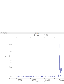
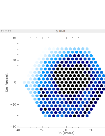
Figure 1: Screen shots of the visualisation windows generated by the view_rss command, on the right the spatial distribution of spaxels, on the left the spectral window showing the spectrum of a particular region of NGC 4625.

Additional information is shown on the IDL terminal where the program was called, a left-click prints the spaxel information including the fibre ID, the offset from the reference spaxel (in arcsec), and if the WCS information is included in the FITS header, it shows the coordinates of the spaxel in sexagesimal and degree units, e.g.

IDL> view_rss, ’pings.n4625_331.fits’

 RSS spectra viewer
 ==================

 Move mouse over the mosaic to plot the spectra

 Options:

   LEFT-click: spaxel information

 MIDDLE-click: selects and stores spaxels by subsequent left-clicks

  RIGHT-click: QUIT


  Spaxel ID    RA offset   Dec offset         RA               Dec            RA deg    Dec deg

       269      17.4200     -12.0779     12h 41m 54.6s    41d 16m 10.8s     190.47765  41.269655
       164     -3.48400      0.00000     12h 41m 52.8s    41d 16m 22.8s     190.46992  41.273010
       267     -8.71893     -21.1184     12h 41m 52.3s    41d 16m  1.7s     190.46799  41.267144
        39      10.4520      12.0779     12h 41m 54.0s    41d 16m 34.9s     190.47507  41.276365

A middle-button click prompts for a PREFIX used to generate a new series of files, all the subsequent left-clicks over the interactive right window will store the position and index of the selected spaxels which are outlined in red. When the program is terminated (by a right-click on the right window) the following files are created:

    Extracted RSS:   PREFIX_rss.fits    (Extracted RSS of the selected spaxels)
   Position table:   PREFIX_pt.txt      (Position table of the new RSS file)
      IDL indices:   PREFIX_index.txt   (Original indices of the selected spaxels)
 Integrated ASCII:   PREFIX_integ.txt   (Integrated spectrum in ASCII format)
  Integrated FITS:   PREFIX_integ.fits  (Integrated spectrum in FITS format)

and the spectral window shows the integrated spectrum of the selected spaxels.

The left panel of Figure 2 shows an example of some selected spaxels from the previous visualisation. The extracted RSS can be visualised again using view_rss, e.g. if the chosen prefix was test1, then the selected spaxels can be displayed by:

IDL> view_rss, ’test1_rss.fits’, ’test1_pt.txt’, /draw

where test1_rss.fits is the new created RSS file and test1_pt.txt is the corresponding position table file, both shown in the right panel of Figure 2.

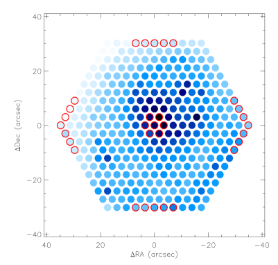
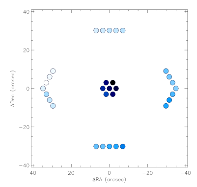
Figure 2: Visualisation examples of spaxel extraction using the middle-click option of the view_rss command. On the left, a single frame of NGC 4625 showing the selected spaxels outlined in red. On the right, visualisation of the selected spaxels by using the view_rss command on the generated RSS and position table files.

Several options are available to better visualise the data, including the central wavelength, width and intensity scaling of the pseudo narrow-band image, different fonts and colour tables, flux intensity and spectral ranges, etc. If the command name of any PINGSoft routine is entered without any keywords, the user will get online help with the correct syntax and available options, e.g.

IDL> view_rss

 CALLING SEQUENCE:

        view_rss, ’RSS.fits’ [, ’pos_table.txt’, MIN_FLUX=min_flux, MAX_FLUX=max_flux, LMIN=lmin, LMAX=lmax, $
                             BAND=band, WIDTH=width, CT=ct, FONT=font, /DRAW, /LINEAR, /GAMMA, /LOG, /ASINH, /PS]


      ’RSS.fits’:  String of the wavelength calibrated RSS FITS file.

 ’pos_table.txt’:  String of the position table of the RSS file in ASCII format (in NE configuration).
                   (compulsory if not included in the default instruments/setups)

    MIN/MAX_FLUX:  Minimum/maximum flux in the spectral window to be plot,
                   if not set these are floating value.

       LMIN/LMAX:  Defines wavelength range on the spectral window,
                   if not set values are taken from the RSS header.

            BAND:  Central wavelength of the narrow band used to display the data,
                   defaults: BAND=6563 (i.e. Halpha) if within the spectral range,
                   else BAND=mean(lambda).

           WIDTH:  Width of the band to display the data, if not set the default is 100 Angstroms.

              CT:  IDL Color Table used to display the data (default ct=1, BLUE/WHITE).

            FONT:  Vector-drawn IDL font to be used, default: 3 (Simplex Roman)

           /DRAW:  Draws the contour of the spaxels.

         /LINEAR:  Displays the range of intensities using a linear min/max scaling.

          /GAMMA:  Displays the range of intensities using a power-law (gamma) scaling.

            /LOG:  Displays the range of intensities using a logarithmic scaling.

          /ASINH:  Displays the range of intensities using an inverse hyperbolic sine function scaling.

             /PS:  Writes a Postscript file of the spaxels visualisation.

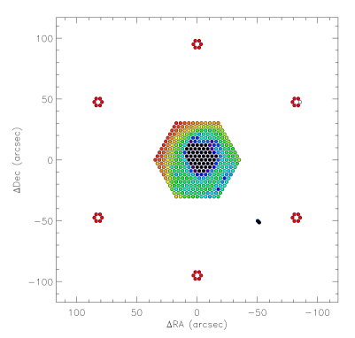
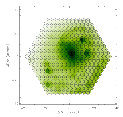
Figure 3: Example of visualisation windows generated by the view_rss command using the /PS option. The left panel corresponds to the full bundle of the PPAK instrument, including the sky and calibration fibres. The right panel corresponds to the dithered mosaic of the nuclear part of NGC 4625. See the text for more details.

If the /PS keyword is set, the program does not display a visualisation on the screen, instead writes a Postscript file of the distribution of spaxels (right window) with the selected display options (see Figure 3).

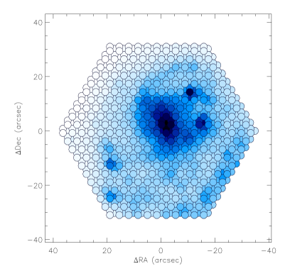
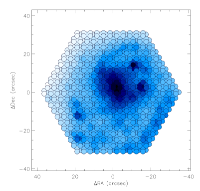
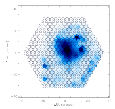
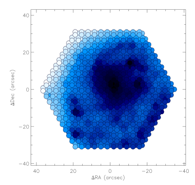
Figure 4: Examples of different visualisations of NGC 4625 generated by the view_rss command using different intensity scaling functions. Top-left panel: a linear scaling, /LINEAR; top-right: a power-law function, /GAMMA; bottom-left: a logarithmic scaling, /LOG, bottom-right: an inverse hyperbolic sine function, /ASINH. See the text for more details.

Intensity scaling

The default colour-scale of the visualisation is obtained by sampling the range of intensities within the chosen narrow band into an ad hoc colour dynamic range of 255 values (i.e. equal to the number of values in a given IDL colour table). However, very different ranges of intensities are expected depending of the object, spectral range and signal-to-noise of the observations. Given that the main purpose of this routine is to visualise easily the IFS data, several intensity scaling functions are available to the user in order to improve the contrast and the identification of spectral features: a full linear (min/max) sampling, a power-law (gamma) function, a logarithmic transformation, and an inverse hyperbolic sine scaling.

For the /GAMMA transformation, the default value is $\gamma=0.7$; for the /LOG scaling, the exponent default value is 2; for the /ASINH function, the default $\beta$ value is 10. For a full explanation of the scaling functions and these parameters see the documentation of the individual routines. Figure 4 shows the visualisation of the dithered mosaic of NGC 4625 using the different intensity scalings mentioned above.

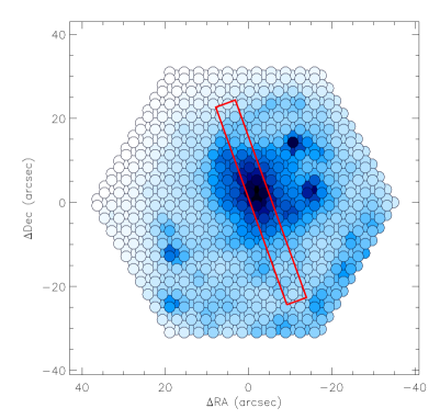
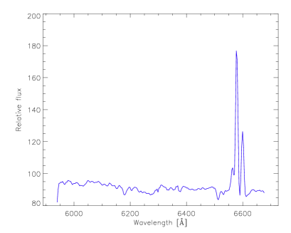
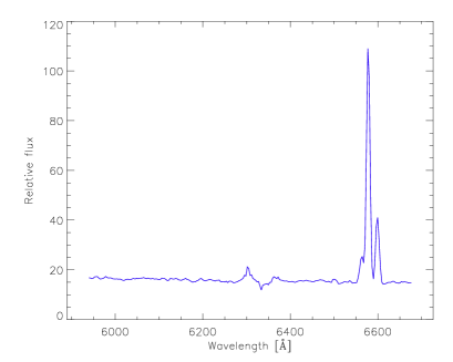
Figure 5: Examples of spectra extraction using a slit aperture (top-left) and a circular aperture (top-right) on the dithered mosaic of NGC 4625, using the extract_slit and extract_aperture respectively. The bottom panels show the integrated spectra extracted within each aperture.

6 PINGSoft list of routines

The main visualisation code in PINGSoft is view_rss, there is an additional routine for visualising specific sections of a RSS file where the ID of the spaxels are known (see below). The rest of the routines in the PINGSoft can be classified into three categories: a) Spectra extraction and integration; b) RSS and FITS manipulation and c) Miscellaneous codes. In this section we include a description of all the available PINGSoft routines, it is beyond the scope of this article to explain every single code and give examples in each case. Detailed descriptions can be found in the documentation.

Visualisation

view_rss: Provides a 2D interactive visualisation of the spaxels and spectra of a RSS file.

view_spaxel: Displays the spectra of previously selected spaxels.

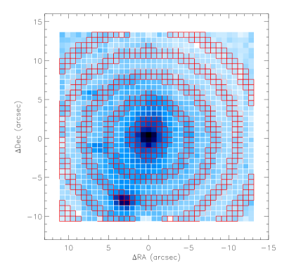
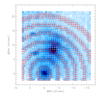
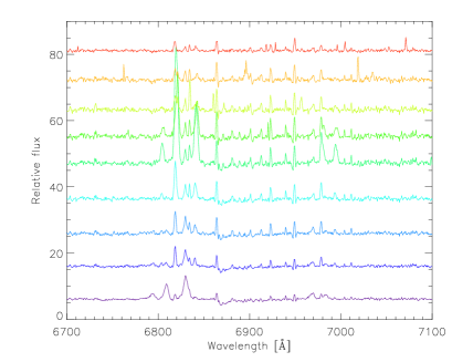
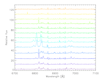
Figure 6: Example of an average radial extraction using both the extract_radial and shift_ptable routines on a VIMOS field of the local LIRG IRAS F06076-2139, after Arribas et al. (2008). Top left-panel: extraction performed at the centre of the field. Top right-panel: extraction performed with a shifted reference point, centered on the nucleus of the South-East galaxy. The bottom panels show the integrated spectra within each ring, with radius increasing from the bottom to top in each case.

Spectra extraction and integration

extract_index: Extracts new a RSS file and generates a new position table based on an index vector.

extract_region: Extracts the spectra of regions selected by hand.

extract_slit: Extracts the spectra within a rectangular aperture, resembling a long-slit observation (see left-panel of Figure 5).

extract_aperture: Extracts the spectra within a circular aperture (see right-panel of Figure 5).

extract_radial: Extracts radial average spectra within consecutive rings from a reference point (see Figure 6).

integrate_rss: Integrates the spectra contained in a RSS file into a single spectrum.

RSS and FITS manipulation

read_rss: Reads a RSS FITS file and stores the data into an IDL vector.

merge_rss: Merges a list of RSS files into a single RSS file.

show_hdr: Shows on screen the header of a FITS file, which can be written to an ASCII file.

write_hdr: Adds or updates an entry in the header of a FITS file, using the fxaddpar.pro utility.

copy_hdr: Copies the header of one FITS file to another.

Miscellaneous codes

cube2rss: Converts a 3D FITS cube with dimensions $X$, $Y$, $\lambda$ to a RSS FITS file + an ad hoc position table in ASCII format.

write_wcs: Adds or updates the WCS (World Coordinate Systems) entries in a FITS header.

get_new_pt: Generates a new position table based on an index of selected spaxels.

shift_ptable: Shifts the reference point or applies an offset to a given position table (an application of this routine is shown in Figure 6).

merge_ptable: Concatenates a list of position table files into a single one for mosaicking purposes.

offset2radec: Transforms small angle offsets in arcsec from a reference point to equatorial coordinates.

radec2offset: Transforms equatorial coordinates to small angle offsets from a given reference point.

7 Summary

The PINGSoft package presented in this article is a set of IDL routines developed for the PINGS project with a special emphasis on visualisation and manipulation of IFS-based data. One of its major advantages with respect other IFS visualisation tools reside in its portability to practically any OS platform with a running version of the IDL data language, a common software in most astronomical research institutes nowadays. The code is completely transparent to the user, allowing to create tailored-based routines depending on each scientific case. The package is run via command lines, which allows more flexibility during repetitive tasks (especially when dealing with large databases), and more precision in some cases (e.g. when defining extraction position/apertures). On the other hand, the spatial and spectral visualisations are fully interactive and optimised for large data files (e.g. mosaics), making the visualisation rendering faster and less prone to errors than other GUI-based visualisation tools.

PINGSoft includes routines to extract regions of interest by hand or within a given geometric aperture, to integrate the spectra within a given region, to convert 3D cubes to the RSS format, to read, edit and write RSS FITS files, and some other miscellaneous codes especially useful in astronomy and spectroscopy. PINGSoft is far from being perfect or complete, the main intention is to help a broad audience to be more familiar with IFS data, but bugs, errors and inconsistencies (especially with instruments not tested so far) are expected. For comments, suggestions and bug reports please contact the author. The PINGSoft package is freely available at:

http://www.ast.cam.ac.uk/research/pings

under the Software section. If you find this package useful on your research, please acknowledge the use of PINGSoft by citing the corresponding reference in your publications. PINGSoft is licensed under GPLv3.

Acknowledgements. I would like to acknowledge the Mexican National Council for Science and Technology (CONACYT) and the Dirección General de Relaciones Internacionales (SEP) for the financial support during the period in which PINGSoft was developed.

References

- Arribas et al. (2008) Arribas, S., Colina, L., Monreal-Ibero, A., Alfonso, J., García-Marín, M., Alonso-Herrero, A., Mar 2008. Vlt-vimos integral field spectroscopy of luminous and ultraluminous infrared galaxies. i. the sample and first results. A&A 479, 687.
- Fevre et al. (1998) Fevre, O. L., Vettolani, G. P., Maccagni, D., Mancini, D., Picat, J. P., Mellier, Y., Mazure, A., Saisse, M., et al., Jul 1998. Virmos: visible and infrared multiobject spectrographs for the vlt. Proc. SPIE Vol. 3355 3355, 8.
- Kelz and Roth (2006) Kelz, A., Roth, M. M., Jun 2006. Experiences with the pmas-ifus. NewAR 50, 355.
- Kelz et al. (2006) Kelz, A., Verheijen, M. A. W., Roth, M. M., Bauer, S. M., Becker, T., Paschke, J., Popow, E., Sánchez, S. F., et al., Jan 2006. Pmas: The potsdam multi-aperture spectrophotometer. ii. the wide integral field unit ppak. PASP 118, 129.
- Rosales-Ortega et al. (2010) Rosales-Ortega, F. F., Kennicutt, R. C., Sánchez, S. F., Díaz, A. I., Pasquali, A., Johnson, B. D., Hao, C. N., Mar 2010. Pings: the ppak ifs nearby galaxies survey. MNRAS, 461.
- Roth et al. (2005) Roth, M. M., Kelz, A., Fechner, T., Hahn, T., Bauer, S.-M., Becker, T., Böhm, P., Christensen, L., et al., Jun 2005. Pmas: The potsdam multi-aperture spectrophotometer. i. design, manufacture, and performance. PASP 117, 620.
- Sánchez (2004) Sánchez, S. F., Mar 2004. E3d, the euro3d visualization tool i: Description of the program and its capabilities. AN 325, 167.
- Sánchez (2006) Sánchez, S. F., Jan 2006. Techniques for reducing fiber-fed and integral-field spectroscopy data: An implementation on r3d. AN 327, 850.
- Sandin et al. (2010) Sandin, C., Becker, T., Roth, M. M., Gerssen, J., Monreal-Ibero, A., Böhm, P., Weilbacher, P., Feb 2010. p3d: a general data-reduction tool for fiber-fed integral-field spectrographs. arXiv 1002, 4406.
- van der Hulst et al. (1992) van der Hulst, J. M., Terlouw, J. P., Begeman, K. G., Zwitser, W., Roelfsema, P. R., Jan 1992. The groningen image processing system, gipsy. Astronomical Data Analysis Software and Systems I 25, 131.
- Verheijen et al. (2004) Verheijen, M. A. W., Bershady, M. A., Andersen, D. R., Swaters, R. A., Westfall, K., Kelz, A., Roth, M. M., Mar 2004. The disk mass project; science case for a new pmas ifu module. AN 325, 151.
- Walsh and Roth (2002) Walsh, J. R., Roth, M. M., Sep 2002. Developing 3d spectroscopy in europe. The Messenger (ISSN 0722-6691) 109, 54.
- Westmoquette et al. (2009) Westmoquette, M. S., Exter, K. M., Christensen, L., Maier, M., Lemoine-Busserolle, M., Turner, J., Marquart, T., May 2009. The integral field spectroscopy (ifs) wiki. arXiv 0905, 3054.