Differential influence of instruments in nuclear core activity evaluation by data assimilation

Abstract

The global activity fields of a nuclear core can be reconstructed using data assimilation. Data assimilation allows to combine measurements from instruments, and information from a model, to evaluate the best possible activity within the core. We present and apply a specific procedure which evaluates this influence by adding or removing instruments in a given measurement network (possibly empty). The study of various network configurations of instruments in the nuclear core establishes that influence of the instruments depends both on the independant instrumentation location and on the chosen network.

Keywords: Data assimilation, neutronic, activities reconstruction, nuclear in-core measurements, data acquisition network

1 Introduction

Data assimilation has been widely developed in earth sciences and especially meteorology. Introducing data assimilation was an important step to improve weather forecasts [1, 2, 3]. Such a technique is now used operationally in all meteorological office. The efficiency of data assimilation for field reconstruction has already been demonstrated in several articles in meteorology [4, 5, 6].

The purpose is to use this technique to make an optimal reconstruction of the activity field in a nuclear core using both measurements and information coming from a numerical model. This approach was also used for nuclear core neutronic state evaluation, and particularly nuclear activity field [7, 8].

In [8], the authors demonstrate how this method is tolerant to instrument loss and that this effect is related to the instrument repartition. The aim of the present article is to go further in the understanding of the instruments location and accuracy effect, and focus more specifically on the individual contribution of each instrument. To achieve this goal, the method is based on the statistical occurrence of instruments with respect to the global quality of the reconstruction associated.

The next section describes the general data assimilation concepts that are used all along this article. Then the parametrisation of data assimilation components are presented in details. From those bases of data assimilation, the specific methodology used to track the individual influence of an instrument on data assimilation is described. Finally, using all previous information, an investigation is done on the instrument location and error modelling effect on the influence of instrument in the core is done.

2 Data assimilation

Here are briefly introduced the useful data assimilation key points to understand their use as applied here [9, 10, 11]. But data assimilation is a wider domain and these techniques are for example the keys of the nowadays meteorological operational forecast [12]. This is through advanced data assimilation methods that the weather forecast has been drastically improved during the last 30 years. Those techniques use all the available data, such as satellite measurements, as well as sophisticated numerical models.

The ultimate goal of data assimilation methods is to estimate the inaccessible true value of the system state, $\mathbf{x}^{t}$ where the $t$ index stands for ”true state” in the so colled ”control space”. The basic idea of most of data assimilation method is to combine information from an a priori on the state of the system (usually called $\mathbf{x}^{b}$, with $b$ for ”background”), and measurements (referenced as $\mathbf{y}^{o}$). The background is usually the result of numerical simulations but can also be derived from any a priori knowledge. The result of data assimilation is called the analysis, denoted by $\mathbf{x}^{a}$, and it is an estimation of the true state $\mathbf{x}^{t}$ researched.

The control and observation spaces are not necessary the same, a bridge between them needs to be build. This is the observation operator $H$ that transform values from the space of the background to the space of observations. For our data assimilation purpose we will use its linearisation $\mathbf{H}$ around the observation values. The inverse operation to go from space of observations to space of the background is given by the transpose $\mathbf{H}^{T}$ of $\mathbf{H}$.

Two other ingredients are necessary. The first one is the covariance matrix of observation errors, defined as $\mathbf{R}=E[(\mathbf{y}^{o}-H(\mathbf{x}^{t})).(\mathbf{y}^{o}-H(\mathbf{x}^{t}))^{T}]$ where $E[.]$ is the mathematical expectation. It can be obtained from the known errors on unbiased measurements which means $E[\mathbf{y}^{o}-H(\mathbf{x}^{t})]=0$. The second one is the covariance matrix of background errors, defined as $\mathbf{B}=E[(\mathbf{x}^{b}-\mathbf{x}^{t}).(\mathbf{x}^{b}-\mathbf{x}^{t})^{T}]$. It represents the error on the a priori state, assuming it to be unbiaised following the $E[\mathbf{x}^{b}-\mathbf{x}^{t}]=0$ no biais property. There are many ways to get this a priori state and background error matrices. However, those matrix are commonly the output of a model and an evaluation of accuracy, or the result of expert knowledge.

It can be proved, within this formalism, that the Best Unbiased Linear Estimator (BLUE) $\mathbf{x}^{a}$, under the linear and static assumptions, is given by the following equation:

$$\mathbf{x}^{a}=\mathbf{x}^{b}+\mathbf{K}\big{(}\mathbf{y}^{o}-H\mathbf{x}^{b}\big{)},$$ (1)

where $\mathbf{K}$ is the gain matrix:

$$\mathbf{K}=\mathbf{B}\mathbf{H}^{T}(\mathbf{H}\mathbf{B}\mathbf{H}^{T}+\mathbf{R})^{-1}.$$ (2)

Moreover, we can get the analysis error covariance matrix $\mathbf{A}$, characterising the analysis errors $\mathbf{x}^{a}-\mathbf{x}^{t}$. This matrix can be expressed from $\mathbf{K}$ as:

$$\mathbf{A}=(\mathbf{I}-\mathbf{K}\mathbf{H})\mathbf{B},$$ (3)

where $\mathbf{I}$ is the identity matrix.

It is worth noting that solving Equation 1 is, if the probability distribution is Gaussian, equivalent to minimise the following function $J(\mathbf{x})$, $\mathbf{x}^{a}$ being the optimal solution:

$$J(\mathbf{x})=(\mathbf{x}-\mathbf{x}^{b})^{T}\mathbf{B}^{-1}(\mathbf{x}-\mathbf{x}^{b})\vskip 6.0pt plus 2.0pt minus 2.0pt+\big{(}\mathbf{y}^{o}-\mathbf{H}\mathbf{x}\big{)}^{T}\mathbf{R}^{-1}\big{(}\mathbf{y}^{o}-\mathbf{H}\mathbf{x}\big{)}.$$ (4)

This minimisation is known in data assimilation as 3D-Var methodology [9].

3 Data assimilation implementation

The framework of this study is the standard configuration of a 900 MWe nuclear Pressurized Water Reactor (PWR900). To perform data assimilation, both simulation code and data are needed. For the simulation code, the EDF experimental calculation code for nuclear core COCAGNE in a standard configuration is used. The description of the basic features of this model are done in Section 3.1.

To have a good understanding of the instrumentation effect on nuclear activity reconstruction, various kind of configurations are studied, even some that do not exist operationally and so cannot be tested experimentally. For that purpose, synthetic data are used, that allows to have an homogeneous approach all along the document. Synthetic data is generated from a model simulation, filtered thought an instrument model and noised according to a predefined measurement error density function (Gaussian type).

Figure 1: The positions of MFC instruments in the nuclear core are localised in assemblies in black within the horizontal slice of the core. The assemblies without instrument are marked in white and the reflector, out of the reactive core, is in gray.

In the present case, we study the activity field reconstruction. An horizontal slice of a PWR900 core is represented on the Figure 1. There is a total of $157$ assemblies within this core. Among those assemblies, $50$ are instrumented with Mobiles Fissions Chambers (MFC). Those assemblies are divided verticaly in $29$ vertical levels. Thus, the size of the control $\mathbf{x}$ to be estimated is $4553$ $(157\times 29)$. The size of the observation vector $\mathbf{y}^{o}$ is $1450$ $(50\times 29)$.

3.1 Brief description of the nuclear core model

The aim of a neutronic code like COCAGNE is to evaluate the neutronic activity field and all associated values within the nuclear core. This field depend on the position in the core and on the neutron energy. To do such an evaluation, the population of neutrons are divided in several groups of energy. In the present case only two groups are taken into account giving the neutronic flux $\Phi=(\Phi_{1},\Phi_{2})$ (even if the present code have no limit for the group number). The material properties depend on the position in the core, as the neutronic flux $\Phi$, identified by solving two-group diffusion equations described by:

$$\left\{\begin{array}[]{l}\displaystyle-\mbox{div}(D_{1}\mbox{{grad}}\Phi_{1})+(\Sigma_{a1}+\Sigma_{r})\Phi_{1}=\frac{1}{k}\Big{(}\nu_{1}\Sigma_{f1}\Phi_{1}+\nu_{2}\Sigma_{f2}\Phi_{2}\Big{)}\\ \displaystyle-\mbox{div}(D_{2}\mbox{{grad}}\Phi_{2})+\Sigma_{a2}\Phi_{2}-\Sigma_{r}\Phi_{1}=0,\\ \end{array}\right.$$ (5)

where $k$ is the effective neutron multiplication factor, all the quantities and the derivatives (except $k$) depend on the position in the core, $1$ and $2$ are the group indexes, $\Sigma_{r}$ is the scattering cross section from group $1$ to group $2$, and for each group, $\Phi$ is the neutron flux, $\Sigma_{a}$ is the absorption cross section, $D$ is the diffusion coefficient, $\nu\Sigma_{f}$ is the corrected fission cross section.

The cross sections also depend implicitly on the concentration of boron, which is a substance added in the water used for the primary circuit to control the neutronic fission reaction, throught a feedback supplementary model. This model takes into account the temperature of the materials and of the neutron moderator, given by external thermal and thermo-hydraulic models. A detailed description of the core physic and numerical solving can be found in reference [13].

The overall numerical resolution consists in searching for boron concentration such that the eigenvalue $k$ is equal to $1$, which means that the nuclear power production is stable and self-sustaining. It is named critical boron concentration computation.

The activity in the core is obtained through a combination of the fluxes $\Phi=(\Phi_{1},\Phi_{2})$, given on the chosen mesh of the core. Using homogeneous materials for each assembly (for example $157$ in a PWR900 reactor), and choosing a vertical mesh compatible with the core (usually $29$ vertical levels), this result in a field of activity of size $157\times 29=4553$ that cover all the core.

3.2 The observation operator $H$

The $H$ observation operator is the composition of a selection and of a normalisation procedure. The selection procedure extracts the values corresponding to effective measurement among the values of the model space. The normalisation procedure is a scaling of the value with respect to the geometry and power of the core. The overall operation is non linear. However, with a range of value compatible with assimilation procedure, we can calculate the linear associated operator $\mathbf{H}$. This observation matrix is a $(4553\times 1450)$ matrix.

3.3 The background error covariance matrix $\mathbf{B}$

The $\mathbf{B}$ matrix represents the covariance between the spatial errors for the the background. The $\mathbf{B}$ matrix is estimated as the product of a correlation matrix $\mathbf{C}$ by a scaling factor to set variances.

The correlation $\mathbf{C}$ matrix is built using a positive function that defines the correlations between instruments with respect to a pseudo-distance in model space. Positive functions have the property (via Bochner theorem) to build symmetric defined positive matrix when they are used as matrix generator [14, 15]. In the present case, Second Order Auto-Regressive (SOAR) function is used to prescribe the $\mathbf{C}$ matrix. In such a function, the amount of correlation depends from the euclidean distance between spatial points. The radial and vertical correlation length ($L_{r}$ and $L_{z}$ respectively, associated to the radial $r$ coordinate and the vertical $z$ coordinate) have different values, which means we are dealing with a global pseudo euclidean distance. The used function can be expressed as follow:

$$C(r,z)=\left(1+\frac{r}{L_{r}}\right)\left(1+\frac{|z|}{L_{z}}\right)\exp{\left(-\frac{r}{L_{r}}-\frac{|z|}{L_{z}}\right)}.$$ (6)

The matrix obtained by the above Equation 6 is a correlation matrix. It is then multiplied by a suitable variance coefficient to get covariance matrix. This coefficient is obtained by statistical study of difference between model and measurements in real case. In real cases, this value is set around a few percent. In our case, the size of the $\mathbf{B}$ matrix is related to the size of model space so it is $(4553\times 4553)$.

3.4 The observation error covariance matrix $\mathbf{R}$

The observation error covariance matrix $\mathbf{R}$ is approximated by a diagonal matrix. It means we assume here that no significant correlation exists between the measurement errors of the MFC. The usual modelling consists on taking the diagonal values as a percentage of the observation values. This can be expressed as:

$$\mathbf{R}_{jj}=\left(\alpha\mathbf{y}^{o}_{j}\right)^{2},\quad\forall j$$ (7)

In our case, the $\alpha$ parameter is fixed according to the accuracy of the measurement and the representative error associated to the instrument, and is the same for all the diagonal coefficients.

This hypothesis of error dependence of the measure amplitude is an usual one. Such an modelling error means that location with a large signal are the one with the higher error. In the following, a constant observation variance is also used. This leads to define the $\mathbf{R}$ matrix diagonal according to the following equation:

$$\mathbf{R}_{jj}=\beta^{2},\quad\forall j$$ (8)

The size of the $\mathbf{R}$ matrix is related to the size of observation space, so it is $(1450\times 1450)$.

4 Method of instrument quality attribution

To evaluate the quality of individual instruments with respect to the estimation of the core activity field, a reference state is needed. This state, denoted by $\mathbf{x}^{a}_{ref}$, corresponds to the data assimilation analysis using all the available instruments. If $\mathbf{x}^{a}$ denotes an analysis experiment performed with less instruments than the maximum available ones, we denote by $\epsilon=||\mathbf{x}^{a}-\mathbf{x}^{a}_{ref}||$ the norm of its difference with the reference analysis. As $\mathbf{x}^{a}_{ref}$ is the best available analysis, we expect that the norm of the difference $\epsilon$ to increase as the number of instrument decreases. The norm $\epsilon$ is thus a measure of the quality of a given experiment.

We consider a set $P$ of $p$ experiments, for instance all those for which a given number of instruments are removed. If $n$ is the maximum number of available instruments and $k$ the fixed number of removed instruments, there are $p=C_{n}^{k}$ experiments in $P$. We then denote by $\epsilon_{i}$, for $i=1,...,p$, the norms of the differences for each experiment with the reference analysis. We can thus plot the histogram of the $\epsilon_{i}$ series. For instance, the histograms corresponding to different choices of $k$ can be compared. The average of the $\epsilon_{i}$ series increases when $p$ increases, since the quality of the analyses decreases when instruments are removed. Its root mean square provides information on the homogeneity of the instrument quality for the field reconstruction.

Dealing with the $\epsilon_{i}$ series can provide information about individual instrument. If we select the $\epsilon_{i}$ values above a fixed threshold, for instance the $10\%$ highest values, we can point out, for each corresponding experiment $i$, the set of instruments which has not been removed. For each instrument, we can count how many times it appears in such an experiment and compare this number to the ones obtained with the other instruments. We can thus assess that an instrument appearing a great number of times in experiments leading to these high values of $\epsilon_{i}$ is of poor quality compared to an instrument which seldom appears for these low quality experiments.

5 Application on various core geometry

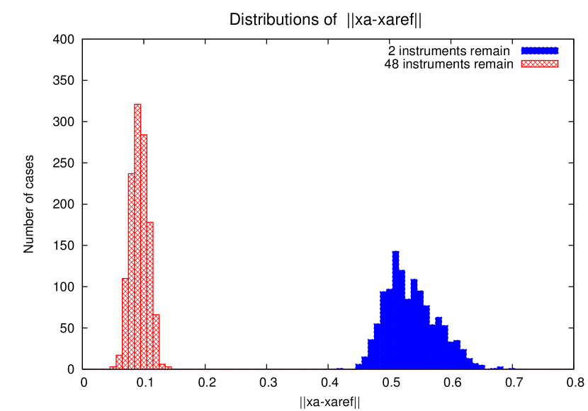
Figure 2: Norm distribution for all the cases where only two instruments are suppressed or remain in the instrument network on a REP900 reactor

First of all, the behaviour of $\epsilon_{i}$ for two extreme cases is examined: when $2$ instruments are removed (i.e. $48$ remain) and when only 2 instruments remain. In both cases, $P$ sets contain $p=1225$ case. This corresponds to all possible combinations to $C^{50}_{2}=C^{50}_{48}=1225$. On Figure 2 are presented the distributions of the $\epsilon_{i}$’s for the cases where two instruments are lost (i.e $48$ remain) or only $2$ remain.

On Figure 2, large differences between the two distributions can be noticed. The shifting of the mean value between those two extreme cases is logical as available information is dramatically changing. Thus the difference of $\epsilon_{i}$ between the two case is changing a lot on the mean. However, the shape of the distribution is also changing. The distribution is a very sharp one when $48$ instruments remain, whereas when only $2$ instruments remain the distribution is broader. The broadening of the distribution shows that the instruments do not have the same influence on the activity field reconstruction. If all instruments have had the same effect on data assimilation, they would have been equivalent. Suppressing whatever instrument would then change the mean value of the distribution of the norm but not the shape. Ideally, this distribution shape should be a very sharp peak. In the present case the distribution when $48$ instruments remain could be a good candidate. Thus if all the instruments where equivalent, only a translation between the distributions of $48$ instruments remains and $2$ instruments remains would have been observed. However, transformation between the two distributions proves that the instruments are not all equivalent.

From that quality measurement, the aim is now to determine the effect of each instrument on the data assimilation results. To archive this goal a detailed study of the distribution of the $\epsilon_{i}$’s is done. Several networks of instruments within the core are considered to obtain an overall understanding of the influence of instruments.

5.1 Standard PWR900 instruments repartition

The first case is a standard PWR900, with data assimilation done as described previously. In this case, the measurement error is proportional to the measure itself as described by Equation 7.

Here are studied the scenarios when only two instruments remain. In such case, the histogram of the $\epsilon_{i}$’s is rather broad, as show in Figure 2. Large distributions (as the one of 2 instruments lost) ensures a better separation of the different classes of instruments that can be present within a given slice in the $\epsilon_{i}$’s values. In a very narrow distribution, as the one where 48 instruments remains of Figure 2, confusion between the different classes associated to a slice in $\epsilon_{i}$ value is more likely.

To quantify the results within a slice of $\epsilon_{i}$ values, first the whole distribution is investigated when no selection on $\epsilon_{i}$ is done. In this case, the distribution of instruments occurrences as defined in Section 4 will be flat. The interesting point for further comparison is its amplitude of $49$ occurrences. This value of amplitude represents $2450=1225\times 2$ coupled references distributed over $50$ instruments. This amplitude gives the reference amount to be compared with a slice of $\epsilon_{i}$ values.

The subset of $10\%$ scenarios that give the highest values is selected to study the influence of instruments among $\epsilon_{i}$ distribution. Assuming an equal influence of all instruments in the $49$ cases, and considering the $10\%$ highest values of $\epsilon_{i}$, the occurence of each instrument should have only a mean value of $4.9$ cases.

The histograms are built according to the method described in Section 4. The result is plotted in Figure 3.

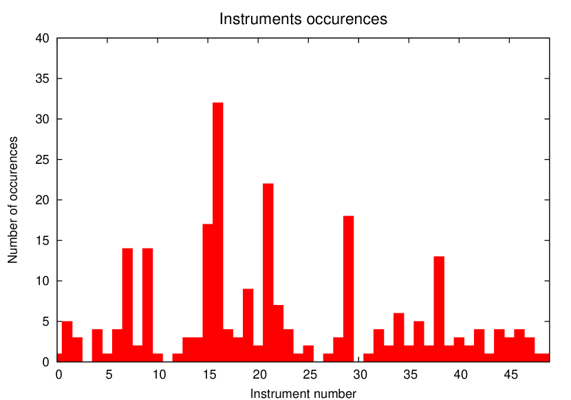
Figure 3: Histogram of the occurrence of the instruments in the $10\%$ scenarios that give the highest values of $\epsilon_{i}$. Each value in abscisse are corresponding to a reference number of one instrument. In ordinate is shown the occurrence of each instrument within remaining instruments list.

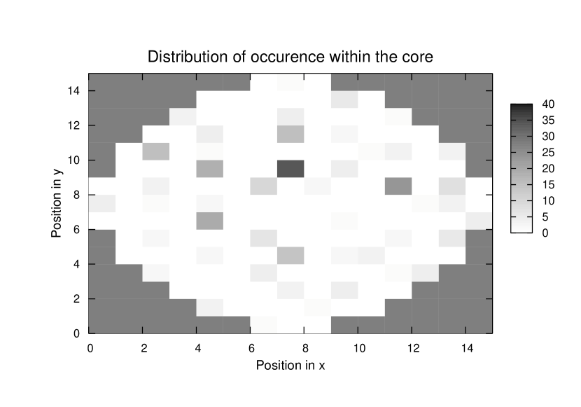
Figure 4: Occurrence of the instruments as a function of their position with in core. The cases kept for doing this histogram are the ones within the $10\%$ highest values of the $\epsilon_{i}$ distribution.

The distribution presented in Figure 3 is not flat, this indicates that the instruments are not equivalent. Moreover the maximum value of occurrence is $32$, which is significantly above the $4.9$ mean value prescribed in the case where all instruments are equivalent. The peaks on Figure 3 are putting in light the instruments that are the least useful for activity field reconstruction. The instruments involved in the low reconstruction quality slice are mainly localised in the centre of the nuclear core as it can be noticed on Figure 4. One hypothesis that can be advanced to explain those differences is the difference of the assembly kind. Looking at the fuel loading pattern we noticed that those effect cannot be explained mainly by the technical specification of the assembly.

This central location of instruments, that are the most present in histogram could be interpreted as a general law. However, the spatial repartition of MFC as show in Figure 1 is complex. Thus, this does not allow to give clear conclusions. However, it worth to notice, comparing Figures 1 and 4, that instruments that are geometrically close do not have necessary the same behaviour. This is the sign of an inner complexity of instrument location effects.

Thus, other configurations need to be investigated to collect more information on this effect. To go further two points need to be considered:

• the hypothesis taken here is to have some measurement error that are proportional to the absolute value of the measurement, as given by Equation 7. This implies that implicit error is higher at location when activity is stronger.

• the instruments repartition is complex. This has the benefit to work in cases that are close to real one. However in the same time it leads to a difficult interpretation.

Thus more theoretical and idealistic configurations need to be considerated to get rid of those both difficulties points and to answer better the question.

5.2 Regular instruments repartition

Figure 5: The MFC instruments within the nuclear core are localised in assemblies in black within the horizontal slice of the core. The assemblies without instrument are marked in white and the reflector is in gray.

To avoid both difficulties presented in previous section, the following instruments configuration is taken:

• a repartition of the instruments within the core following a Cartesian map. The location of the instruments within such a configuration is reported on the Figure 5. Within this configuration, only $40$ MFC are available. This number of instruments is a bit lower than the $50$ of the standard PWR900 case presented in Figure 1. It leads to an overall difference in instruments density and quality of initial reconstruction.

• Measurement errors are taken as constant, as described by Equation 8.

If only the hypothesis on geometry presented above is kept, the overall conclusion of this section is not changed at all. This second hypothesis on measurement error modelling, whatever is the instrument location choice, has low effect on the results.

Using both above hypothesis for the calculation, the same study as the one done for standard configuration, is done here. The analysis is done according to method described in Section 4. In the present case the value of $\mathbf{x}^{a}_{ref}$ is not the same as in the standard case described in Section 5.1. This new value of $\mathbf{x}^{a}_{ref}$ is calculated assuming all the $40$ instruments are localised according to Figure 5. Within such a configuration there are $C^{40}_{2}=780$ possible scenarios when $2$ instruments remain, so all configurations are evaluated.

If all the cases are taken into account, an uniform distribution is obtained. The amplitude of this distribution is $39$. This value represent $1560=780\times 2$ coupled references distributed over $40$ instruments. This means that, for a selection of $10\%$ of the scenarios the mean flat value is around $4.0$. This value is a reference to compare with the values obtained in occurrence distribution within a slice of value of $\mathbf{x}^{a}-\mathbf{x}^{a}_{ref}$.

As in Section 5.1, the ensemble of scenarios that leads to the $10\%$ highest $\mathbf{x}^{a}-\mathbf{x}^{a}_{ref}$ values are investigated. The occurrence of the instruments for the scenarios giving the $10\%$ highest $\mathbf{x}^{a}-\mathbf{x}^{a}_{ref}$ values are plotted in Figure 6.

The peaks in Figure 6 within the distribution prove that the instruments are not equivalent, even in the case of a regular repartition of instruments according to a Cartesian grid. This confirms that all instruments do not have the same effect, whatever is the chosen network. Another point is the quasi symmetry of the distribution with respect to the mean of the chosen numbering. The numbering of the instruments is done from right to left and from top to bottom. Which means that the instruments numbered $1$ at the top left is equivalent to the one numbered $40$ at the bottom right. This classification lead to equivalence between the instruments numbered from $1$ to $20$ with the corresponding one, respectively, between $40$ and $21$. Thus symmetry imposed by numbering appears in the histogram. Moreover, even if a fixed value of the measurement error is imposed, this do not eliminate the effect of location on the instruments. This location effect is then rather dominant with respect to the error effect. To have a better view on a plan of those instruments, their spatial locations within the core are represented in Figure 7.

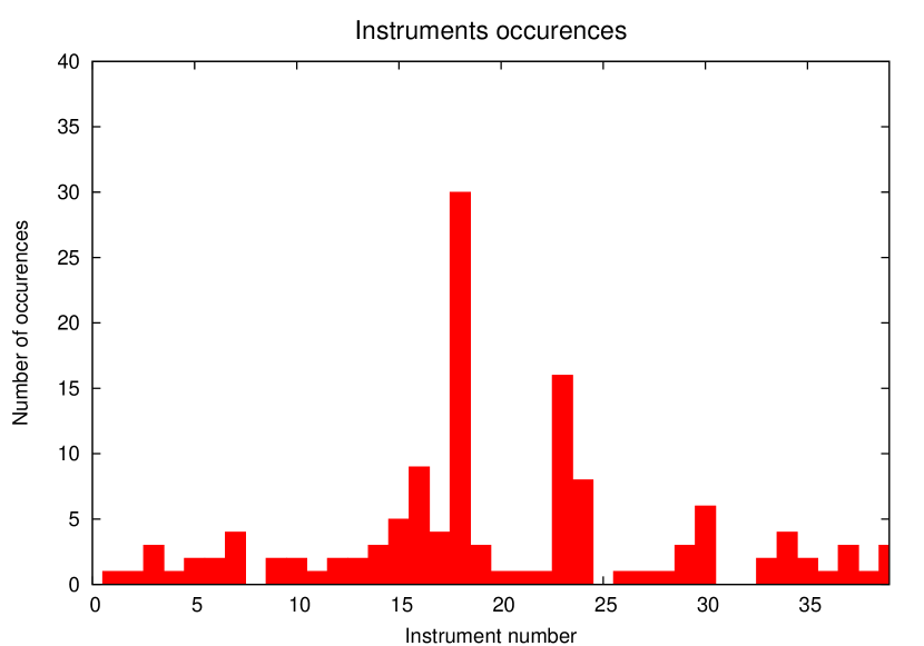
Figure 6: Histogram of the occurrence of the instruments in the $10\%$ scenarios that give the highest values of $\epsilon_{i}$. Each value in abscisse is corresponding to a reference number of one instrument. In ordinate is shown the occurrence of the instruments within remaining instruments list.

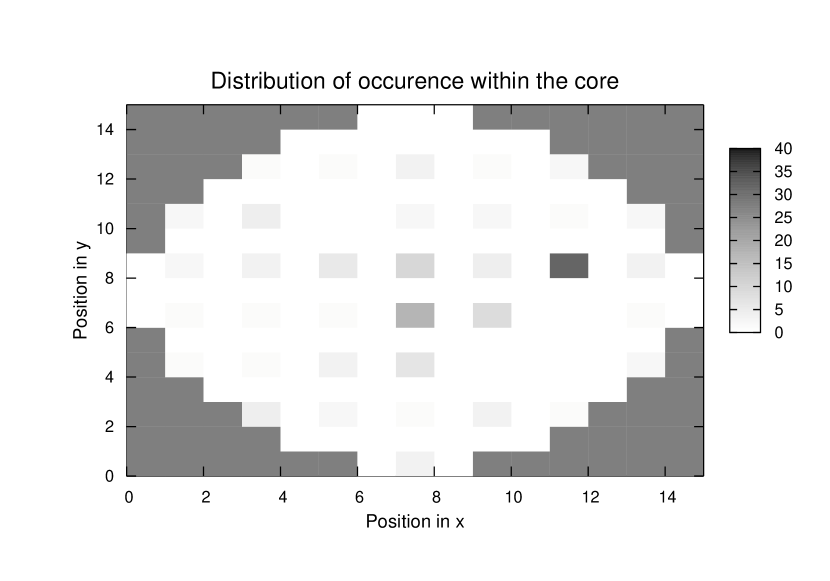
Figure 7: Occurrence of the instruments as a function of their position within the core. The cases kept for doing this histogram are the ones within the $10\%$ highest values of the $\epsilon_{i}$ distribution.

Figure 7 shows the instruments that have a low contribution to the field reconstruction with data assimilation. Those instruments are mainely localised in the centre of the core. In this case this interpretation is easy as the instruments location are distributed regularly as shown in Figure 5. This central location of the instruments confirms what was seen in Figure 6 about the central instruments locations.

Beyond this global similitude, several differences are notable comparing Figure 7 and Figure 4. In Figure 7, the most represented instrument is located in the top middle of the core centre. However, in Figure 6, this instrument is located on the right side of the core. This effect of location changing, on the most represented instrument, can be attributed to the global difference between available instruments positions as measurement error repartition and assembly technical specifications hypothesis can be excluded. No effect of the modelling of the error respect to Equation 7 or Equation 8 can be seen whatever is used. The repetition of the assembly is exactly the same as in standard case and the assembly technical characteristics are not correlated directly to the results.

The conclusion from that point is that locations of the most influential instruments are dominated by the instrumental network pattern chosen for the core. Moreover, the precise location of the most represented instrument can be put in light precisely using statistics on the occurrence of each instrument in specific slice of $\epsilon_{i}$ norm values. In the study presented in Section 5.1 and 5.2, both are assuming that two instruments are added to a non instrumented core. This kind of hypothesis is rather strong and do not allows to conclude in a more general case.

From present step, it seems that the instruments located at the centre are the most represented in the $10\%$ highest $\epsilon_{i}$ values. In this sense, they lead to the worth reconstruction of the core, which seem very paradoxal. To understand that point, it is necessary to keep in mind that within a data assimilation procedure, the measurement provided by an instrument have influence within a rather large radius around the measure itself. This comes from the construction on the $\mathbf{B}$ matrix that is presented in Equation 6. Typically, this matrix is constructed with an influence length of few assemblies. Thus, the improvement through data assimilation is driven by the few measurements that can generated too large modification, that are not optimum on close assemblies. This does not lead to a overall quality improvement of the final analysis.

Such an effect means that it is necessary to have more instruments in the starting network to make a better balance between information they provide. To confirm this hypothesis, the amplitude of the highest peak in Figure 6 give enough information. This plot correspond to the occurrence of a given instruments in the $10\%$ higher value of $\mathbf{x}^{a}-\mathbf{x}^{a}_{ref}$ norm. On Figure 6 maximum peak value is $30$. This value is $23\%$ lower than the flat limit when no selection is done at $39$. This mean that in $23\%$ of the cases, there are a counter balancing of the overconfidenced information given by one instrument. Thus, the influence of other instruments in the network must be considered.

5.3 Half instrumented core with regular repartition

The aim of this section is to comfort conclusions on the influence of starting instrumental network configuration obtained in Section 5.1 and 5.2. To keep the advantage of the flat error and regular distribution new case is build on those basis. The assumption that the core is half instrumented will be done in this part. This means that one half will be considered as fixed one. Then only instruments coming from the other half are added.

To keep the regularity of the distribution, instruments are separated in the fixed or removable categories alternatively using as basis the regular distribution presented in Section 5.2. Thus, two categories of $20$ instruments each are obtained. The location of the instruments for each category is presented on Figure 8. This process to build classes, even if it leads to some asymmetry, allows on overall to keep the convenient regularity features of the initial repartition.

Figure 8: The MFC instruments within the nuclear core are localised in assemblies in black with in the horizontal slice of the core. The assemblies without instrument are marked in white and the reflector is in gray. The left picture is for the instruments that are always kept. The right figure represent instruments that may be suppressed.

Thus, an addition of $2$ instruments from the removable set is done to the set of $20$ fixed instruments. As only $20$ instruments remains the number of possible scenarios is smaller than in Section 5.1 and 5.2 remain. In this case, there are only $C^{2}_{20}$ cases which means $190$ possibilities. As expected, the norm distribution of $\mathbf{x}^{a}-\mathbf{x}^{a}_{ref}$ is a narrower that the previous case. This distribution, contrary to the one presented for two instruments remaining in Figure 2, is rather symmetric. Still the distribution is board enough to make a cut over the $10\%$ higher values of the distribution.

To get a clear view of the instruments, we will make occurrence histogram taking into account only the two instruments that are added. However we will still working in the framework of all instruments set. This new configuration will be analysed according to the method used in Section 5.1 and 5.2.

In the present case only half of the instruments are considered. Thus the plot of occurrence on all the studied scenarios is a sampling function as only the locations with a removable instrument are considered. The frequency of this sampling function is $1/2$ instrument. This characteristic frequency comes from the regular alternative sorting of instruments either in removable set of instruments either in fixed set of instruments. The amplitude of this sampling function is $19$ which correspond to $190\times 2$ divided by the $20$ possibles locations. In this case, this is the difference respect of this sampling function that will be studied. As previously, this is the $10\%$ higher value of norm of $\mathbf{x}^{a}-\mathbf{x}^{a}_{ref}$ distribution that are investigated. The results of the instruments occurrence histogram are plotted on Figure 10. For this $10\%$ subset of instruments, the hypothesis of independence of instruments would leads to an histogram of occurrence as a sampling function of frequency $1/2$ and mean amplitude of $1.9$

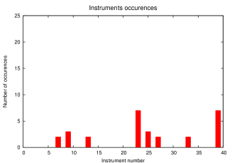
Figure 9: Histogram of the occurrence of instruments for the $10\%$ highest values of the $\epsilon_{i}$ distribution. Each value in abscisse are corresponding to a reference number of one instrument. In ordinate is shown the occurrence of the instruments within remaining instruments list.

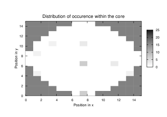
Figure 10: Occurrence of the instruments as a function of their position with in core. The cases kept for doing this histogram are the ones within the $10\%$ highest values of the $\epsilon_{i}$ distribution.

In Figure 10 the pattern of occurrence is not any more a sampling function with a constant amplitude but some peaks appear. The amplitude of the most important peak are around $7$ which is far beyond the mean value of the regular sampling function that is $1.9$. Such a huge amplitude peak signs one more time the non equivalence of all the instruments within the data assimilation procedure. No more symmetry exists in the histogram comparing to Figure 6 and this is even asymmetry that appears. This an interesting change as the instruments selection method should keep some how this symmetry. This sign an influence of the existing instruments network on data assimilation results.

The precise spatial location of the instruments is reported in Figure 10. Comparing the location of the instruments in Figure 10 respect to the case of regular repartition for the same kind of slice in $\mathbf{x}^{a}-\mathbf{x}^{a}_{ref}$ presented in Figure 7 several differences are obvious.

The most interesting point is that in the present case presented in Figure 10 a peak arise at the very bottom of the core. Thus, the MFC that got the lowest influence on reconstruction by data assimilation are in this case not any more localised in the centre of the core. This show one more time a significant difference with results obtained especially in Section 5.2 that is dealing with a very close initial configuration.

Even if the same instrument locations are used originally, those results are very different from the ones presented in Figure 7. Thus we see that both the original present instrumentation as well as the location of the instruments have an effect on the activity field reconstruction quality.

Examining together Figures 4, 10 and 7, we can notice that the instruments that are the least important often seem to be localised in area where the density of instruments present or potentially available is fairly large.

6 Conclusion

One of the purpose of this study was to make a study of the influence of the instruments within a data assimilation procedure to reconstruct activity in nuclear core. The quality of reconstruction is evaluated thought the norm of $\mathbf{x}^{a}-\mathbf{x}^{a}_{ref}$ for all the possible combination of two instruments addition that is the best case in terms of statistic and analysis of the results.

Focusing on the instruments leading to the $10\%$ highest value of $\epsilon_{i}$ when instruments are added to a non instrumented core of PWR900, it can be noticed that they are not equivalent. It appears that within a distribution that is supposed to be flat if all instrument play the same role, some instruments have higher occurrence than other.

This effect can be understood focusing on a Cartesian regular repartition of the instruments. Within this regular configuration, it was shown that the instruments localised in the centre are the least important for activity field reconstruction with data assimilation. This proves that the instruments location is the most important factor that impact the quality reconstruction with data assimilation.

To better understand the effect of adding instruments to a system, we choose to do do the same procedure starting from a core with a half instrumented regular distribution. Through this study, it can be demonstrated that the locations in the center of the least influential instruments is not a general rule.

Within those studies, it is determined, empirically, that the influence of the instruments is related to the density of the present or potentially available instruments around this location.

The determination of the worst instruments (respectively the best) to add to an measurement system, to improve data assimilation with it, is depending on several parameters.

The starting instrumental configuration to which instruments need to be added play a fundamental role. It was proven here that results are very different when instruments are added to a non instrumented system than to a partially (half) instrumented one. Such a non equivalence respect to starting point proves that building a complete instrumental system cannot be done iteratively. Such a system will have limited efficiency as each step is dependant of the previous and not of the global situation.

This imply that, in order to build an optimal measurement network in a nuclear core, it is necessary to be able to take into account all the instruments globally.

Developing tools and diagnostic for a determination of such optimal network is then complex. This is especially true when a lot of measurement are needed. Moreover such a goal can only be achieved through advanced mathematical study and powerful computing usage.

References

- [1] David F. Parrish and John C. Derber. The national meteorological center’s spectral statistical interpolation analysis system. Monthly Weather Review, 120:1747–1763, 1992.
- [2] Ricardo Todling and Stephen E. Cohn. Suboptimal schemes for atmospheric data assimilation based on the kalman filter. Monthly Weather Review, 122:2530–2557, 1994.
- [3] Kayo Ide, Philippe Courtier, Michael Ghil, and Andrew C. Lorenc. Unified notation for data assimilation: operational, sequential and variational. Journal of the Meteorological Society of Japan, 75(1B):181–189, 1997.
- [4] S. M. Uppala and et al. The ERA-40 re-analysis. Quaterly Journal of the Royal Meteorological Society, 131(612, Part B):2961–3012, 2005.
- [5] E. Kalnay and et al. The NCEP/NCAR 40-year reanalysis project. Bulletin of American Meteorological Society, 77:437–471, 1996.
- [6] G. J. Huffman and et al. The global precipitation climatology project (GPCP) combined precipitation dataset. Bulltin of American Meteorological Society, 78:5–20, 1997.
- [7] Sébastien Massart, Samuel Buis, Patrick Erhard, and Guillaume Gacon. Use of 3DVAR and Kalman filter approaches for neutronic state and parameter estimation in nuclear reactors. Nuclear Science and Engineering, 155(3):409–424, 2007.
- [8] Bertrand Bouriquet, Jean-Philippe Argaud, Patrick Erhard, Guillame Gacon, Sébastien Massart, and Sophie Ricci. Robustness of nuclear core activity reconstruction by data assimilation (submited), 2010.
- [9] Olivier Talagrand. Assimilation of observations, an introduction. Journal of the Meteorological Society of Japan, 75(1B):191–209, 1997.
- [10] Eugenia Kalnay. Atmospheric Modeling, Data Assimilation and Predictability. 2003.
- [11] Fran ois Bouttier and Philippe Courtier. Data assimilation concepts and methods. Meteorological training course lecture series, ECMWF, March 1999.
- [12] F. Rabier, H. Järvinen, E. Kilnder, J.F. Mahfouf, and A. Simmons. The ECMWF operational implementation of four-dimensional variational assimilation. part I: Experimental results with simplified physics. Quarterly Journal of the Royal Meteorological Society, 126:1143–1170, 2000.
- [13] James J. Duderstadt and Louis J. Hamilton. Nuclear reactor analysis. John Wiley & Sons, 1976.
- [14] Georges Matheron. La théorie des variables régionalisées et ses applications. Cahiers du Centre de Morphologie Mathématique de l’ENSMP, Fontainebleau, Fascicule 5, 1970.
- [15] Denis Marcotte. Géologie et géostatistique minières (cours), 2008.