Tight and simple Web graph compression

Abstract

Analysing Web graphs has applications in determining page ranks, fighting Web spam, detecting communities and mirror sites, and more. This study is however hampered by the necessity of storing a major part of huge graphs in the external memory, which prevents efficient random access to edge (hyperlink) lists. A number of algorithms involving compression techniques have thus been presented, to represent Web graphs succinctly but also providing random access. Those techniques are usually based on differential encodings of the adjacency lists, finding repeating nodes or node regions in the successive lists, more general grammar-based transformations or 2-dimensional representations of the binary matrix of the graph. In this paper we present two Web graph compression algorithms. The first can be seen as engineering of the Boldi and Vigna (2004) method. We extend the notion of similarity between link lists, and use a more compact encoding of residuals. The algorithm works on blocks of varying size (in the number of input lines) and sacrifices access time for better compression ratio, achieving more succinct graph representation than other algorithms reported in the literature. The second algorithm works on blocks of the same size, in the number of input lines, and its key mechanism is merging the block into a single ordered list. This method achieves much more attractive space-time tradeoffs.

raph compression, random access

1 Introduction

Development of succinct data structures is one of the most active research areas in algorithmics in the last years. A succinct data structure shares the interface with its classic (non-succinct) counterpart, but is represented in much smaller space, via data compression. Successful examples along these lines include text indexes [25], dictionaries, trees [24, 15] and graphs [24]. Queries to succinct data structures are usually slower (in practice, although not always in complexity terms) than using non-compressed structures, hence the main motivation in using them is to allow to deal with huge datasets in the main memory. For example, indexed exact pattern matching in DNA would be limited to sequences shorter than 1 billion nucleotides on a commodity PC with 4 GB of main memory, if the indexing structure were the classic suffix array (SA), and even less than half of it, if SA were replaced with a suffix tree. On the other hand, switching to some compressed full-text index (see [25] for a survey) shifts the limit to over 10 billion nucleotides, which is more than enough to handle the whole human genome.

Another huge object of significant interest seems to be the Web graph. This is a directed unlabeled graph of connections between webpages (i.e., documents), where the nodes are individual HTML documents and the edges from a given node are the outgoing links to other nodes. We assume that the order of hyperlinks in a document is irrelevant. Web graph analyses can be used to rank pages, fight Web spam, detect communities and mirror sites, etc.

As of early Sept. 2011, it is estimated that Google’s index has about 44 billion webpages. Assuming 20 outgoing links per node, 5-byte links (4-byte indexes to other pages are simply too small) and pointers to each adjacency list, we would need more than 4.4 TB of memory, ways beyond the capacities of the current RAM memories. We believe that, confronted with the given figures, the reader is now convinced about the necessity of compression techniques for Web graph representation.

Preliminary versions of this manuscript were published in [16] and [17].

2 Related work

We assume that a directed graph $G=(V,E)$ is a set of $n=|V|$ vertices and $m=|E|$ edges. The earliest works on graph compression were theoretical, and they usually dealt with specific graph classes. For example, it is known that planar graphs can be compressed into $O(n)$ bits [28, 18]. For dense enough graphs, it is impossible to reach $o(m\log n)$ bits of space, i.e., go below the space complexity of the trivial adjacency list representation. Since the seminal Jacobson’s thesis [20] on succinct data structures, there appear papers taking into account not only the space occupied by a graph, but also access times.

There are several works dedicated to Web graph compression. Bharat et al. [4] suggested to order documents according to their URL’s, to exploit the simple observation that most outgoing links actually point to another document within the same Web site. Their Connectivity Server provided linkage information for all pages indexed by the AltaVista search engine at that time. The links are merely represented by the node numbers (integers) using the URL lexicographical order. We noted that we assume the order of hyperlinks in a document irrelevant (like most works on Web graph compression do), hence the link lists can be sorted, in ascending order. As the successive numbers tend to be close, differential encoding may be applied efficiently.

Randall et al. [27] also use this technique (stating that for their data 80% of all links are local), but they also note that commonly many pages within the same site share large parts of their adjacency lists. To exploit this phenomenon, a given list may be encoded with a reference to another list from its neighborhood (located earlier), plus a set of additions and deletions to/from the referenced list. Their encoding, in the most compact variant, encodes an outgoing link in 5.55 bits on average, a result reported over a Web crawl consisting of 61 million URL’s and 1 billion links.

One of the most efficient compression schemes for Web graph was presented by Boldi and Vigna [7] in 2003. Their method is likely to achieve around 3 bits per edge, or less, at link access time below 1 ms at their 2.4 GHz Pentium4 machine. Of course, the compression ratios vary from dataset to dataset. We are going to describe the Boldi and Vigna algorithm in detail in the next section as this is the main inspiration for our solution.

Claude and Navarro [11, 13] took a totally different approach of grammar-based compression. In particular, they focus on Re-Pair [22] and LZ78 compression schemes, getting close, and sometimes even below, the compression ratios of Boldi and Vigna, while achieving much faster access times. To mitigate one of the main disadvantages of Re-Pair, high memory requirements, they developed an approximate variant of this algorithm.

When compression is at a premium, one may acknowledge the work of Asano et al. [3] in which they present a scheme creating a compressed graph structure smaller by about 20–35% than the BV scheme with extreme parameters (best compression but also impractically slow). The Asano et al. scheme perceives the Web graph as a binary matrix (1s stand for edges) and detects 2-dimensional redundancies in it, via finding six types of blocks in the matrix: horizontal, vertical, diagonal, L-shaped, rectangular and singleton blocks. The algorithm compresses the data of intra-hosts separately for each host, and the boundaries between hosts must be taken from a separate source (usually, the list of all URL’s in the graph), hence it cannot be justly compared to other algorithms mentioned here. Worse, retrieval times per adjacency list are much longer than for other schemes: on the order of a few milliseconds (and even over 28 ms for one of three tested datasets) on their Core2 Duo E6600 (2.40 GHz) machine running Java code. We note that 28 ms is at least twice more than the access time of modern hard disks, hence working with a naïve (uncompressed) external representation would be faster for that dataset (on the other hand, excessive disk use from very frequent random accesses to the graph can result in a premature disk failure). It seems that the retrieval times can be reduced (and made more stable across datasets) if the boundaries between hosts in the graph are set artificially, in more or less regular distances, but then also the compression ratio is likely to drop.

Also excellent compression results were achieved by Buehrer and Chellapilla [9], who used grammar-based compression. Namely, they replace groups of nodes appearing in several adjacency lists with a single “virtual node” and iterate this procedure; no access times were reported in that work, but according to findings in [12] they should be rather competitive and at least much shorter than of the algorithm from [3], with compression ratio worse only by a few percent.

Apostolico and Drovandi [2] proposed an alternative Web graph ordering, reflecting their BFS traversal (starting from a random node) rather than traditional URL-based order. They obtain quite impressive compressed graph structures, often by 20–30% smaller than those from BV at comparable access speeds. Interestingly, the BFS ordering allows to handle the link existential query (testing if page $i$ has a link to page $j$) almost twice faster than returning the whole neighbor list. Still, we note that using non-lexicographical ordering is harmful for compact storing of the webpage URLs themselves (a problem accompanying pure graph structure compression in most practical applications). Note also that reordering the graph is the approach followed in more recent works from the Boldi and Vigna team [6, 5].

Anh and Moffat [1] devised a scheme which seems to use grammar-based compression in a local manner. They work in groups of $h$ consecutive lists and perform some operations to reduce their size (e.g., a sort of 2-dimensional RLE if a run of successive integers appears on all the $h$ lists). What remains in the group is then encoded statistically. Their results are very promising: graph representations by about 15–30% (or even more in some variant) smaller than the BV algorithm with practical parameter choice (in particular, Anh and Moffat achieve 3.81 bpe and 3.55 bpe for the graph EU) and report comparable decoding speed. Details of the algorithm cannot however be deduced from their 1-page conference poster.

Recent works focus on graph compression with support for bidirectional navigation. To this end, Brisaboa et al. [8] proposed the $k^{2}$-tree, a spatial data structure, related to the well-known quadtree, which performs a binary partition of the graph matrix and labels empty areas with 0s and non-empty areas with 1s. The non-empty areas are recursively split and labeled, until reaching the leaves (single nodes). An important component in their scheme is an auxiliary structure to compute rank queries [20] efficiently, to navigate between tree levels. It is easy to notice that this elegant data structure supports handling both forward and reverse neighbors, which implies from its symmetry. Ladra [21] proposed a more efficient encoding of leaves (which are boxes of sizes e.g. $8\times 8$ rather than single bits) in this scheme, making use of a common vocabulary for the different leaf submatrices and directly addressable codes. Very recently, on the base of the mentioned encoding, Claude and Ladra [10] achieved even better results, and the key idea was to divide the original square matrix into subdomains, cutting out several non-overlapping squares (subgraphs) along the diagonal of the binary matrix; each generated subgraph is stored independently. Experiments show that even the original work uses significantly less space (3.3–5.3 bits per link) than the Boldi and Vigna scheme applied for both direct and transposed graph, at the average neighbor retrieval times of 2–15 microseconds (Pentium4 3.0 GHz). The Claude and Ladra variant reduces the space to about 3–4 bits per link and the retrieval time is improved to about 1 microsecond or less (Intel Xeon 2.0 GHz).

In other recent work, Claude and Navarro [12] showed how Re-Pair can be used to compress the graph binary relation efficiently, enabling also to extract the reverse neighbors of any node. These ideas let them achieve a number of Pareto-optimal space-time tradeoffs, usually competitive to those from the (original variant of the) $k^{2}$-tree.

Finally, we have to mention the Hernández and Navarro work [19], where they combine their previous techniques, $k^{2}$-tree [8] and Re-Pair for compressing the graph binary relation [12] with edge reducing [9], obtaining interesting trade-offs. In particular, if some of the access time can be sacrified, the space they achieved is the smallest known among the solutions supporting bidirectional queries.

3 The Boldi and Vigna scheme

Based on WebGraph datasets (http://webgraph.dsi.unimi.it/), Boldi and Vigna noticed that similarity is strongly concentrated; typically, either two adjacency (edge) lists have nothing or little in common, or they share large subsequences of edges. To exploit this redudancy, one bit per entry on the referenced list could be used, to denote which of its integers are copied to the current list, and which are not. Those bit-vectors are dubbed copy lists. Still, Boldi and Vigna go further, noticing that copy lists tend to contain runs of 0s and 1s, thus they compress them using a sort of run-length encoding. They assume the first run consists of 1s (if the copy list actually starts with 0s, the length of the first run is simply zero), and then it allows to represent a copy list as only a sequence of run lengths, encoded e.g. with Elias coding.

The integers on the current list which didn’t occur on the referenced list must be stored too, and how to encode them is another novelty of the described algorithm. They detect intervals of consecutive (i.e., differing by 1) integers and encode them as pairs of the left boundary and the interval length; the left boundary of the next interval on a given list will be encoded as the difference to the right boundary of the previous interval minus two (this is because between the end of one interval and the beginning of another there must be at least one integer). The numbers which do not fall into any interval are called residuals and are also stored, encoded in a differential manner.

Finally, the algorithm allows to select as the reference list one of several previous lines; the size of the window is one of the parameters of the algorithm posing a tradeoff between compression ratio and compression/decompression time and space. Another parameter affecting the results is the maximum reference count, which is the maximum allowed length of a chain of lists such that one cannot be decoded without extracting its predecessor in the chain.

4 Our algorithms

We present two approaches to Web graph compression working locally, in small blocks; the first one usually reaches slightly higher compression ratios but the second is more practical, as being much faster.

4.1 An algorithm based on similarity of successive lists

Our first algorithm (Alg. 1, SSL stands for “similarity of successive lists”) works in blocks consisting of multiple adjacency lists. The blocks in their compact form are approximately equal, which means that the number of adjacency lists per block varies; for example, in graph areas with dominating short lists the number of lists per block is greater than elsewhere.

We work in two phases: preprocessing and final compression, using a general-purpose compression algorithm. The algorithm processes the adjacency lines one-by-one and splits their data into two streams.

1	$firstLine\leftarrow\mbox{{true}}$
2	$prev\leftarrow$ [ ]
3	$outB\leftarrow$ [ ]
4	$outF\leftarrow$ [ ]
5	for $line\in G$ do
6		$residuals\leftarrow line$
7		if $firstLine=\mbox{{false}}$ then
8			$f[1\ldots|prev|]\leftarrow[1,1,\ldots,1]$
9			for $i\leftarrow 1$ to $|prev|$ do
10				if $prev[i]\in line$ then $f[i]\leftarrow 0$
11				else if $prev[i]+1\in line$ then $f[i]\leftarrow 2$
12				else if $prev[i]+2\in line$ then $f[i]\leftarrow 3$
13			append($outF$, $f$)
14			for $i\leftarrow 1$ to $|prev|$ do
15				if $f[i]\neq 1$ then
16					remove($residuals$, $prev[i]$)
17		$residuals^{\prime}\leftarrow$ RLE(diffEncode($residuals$)) + [0]
18		append($outB$, byteEncode($residuals^{\prime}$))
19		$prev\leftarrow line$
20		$firstLine\leftarrow\mbox{{false}}$
21		if $|outB|\geq BSIZE$ then
22			compress($outB$)
23			compress($outF$)
24			$outB\leftarrow$ [ ]
25			$outF\leftarrow$ [ ]
26			$firstLine\leftarrow\mbox{{true}}$

Alg. 1 GraphCompressSSL($G,BSIZE$).

One stream holds copy lists, in an extended sense compared to the Boldi and Vigna solution. Our copy lists are no longer binary but consist of four different flag symbols: 0 denotes an exact match (i.e., value $j$ from the reference list occurs somewhere on the current list), 2 means that the current list contains integer $j+1$, 3 means that the current list contains integer $j+2$, if the corresponding integer from the reference list is $j$. Finally, the bits 1 correspond to the items from the reference list which have not been earlier labeled with 0, 2 or 3.

Of course, several events may happen for a single element, e.g., the integer 34 from the reference list triggers three events if the current list contains 34, 35 and 36. In such case, the flag with the smallest value is chosen (i.e., 0 in our example).

Moreover, we make things even simpler than in the Boldi–Vigna scheme and our reference list is always the previous adjacency list.

The other stream stores residuals, i.e., the values which cannot be decoded with flags 0, 2 or 3 on the copy lists. First differential encoding is applied and then an RLE compressor for differences 1 only (with minimum run length set experimentally to 5) is run. The resulting sequence is terminated with a unique value (0) and then encoded using a byte code.

For this last step, we consider two variants. One is similar to two-byte dense code [26] in spending one bit flag in the first codeword byte to tell the length of the current codeword. Namely, we choose between 1 and $b$ bytes for encoding each number, where $b$ is the minimum integer such that $8b-1$ bits are enough to encode any node value in a given graph. In practice it means that $b=3$ for EU and $b=4$ for the remaining available datasets.

The second coding variant can be classified as a prelude code [14] in which two bits in the first codeword byte tell the length of the current codeword; originally the lengths are 1, 2, 3 and 4 but we take 1, 2 and $b$ such that $8b-2$ bits are enough to encode the largest value in the given graph (i.e., $b$ could be 5 or 6 for really huge graphs).

Once the residual buffer reaches at least BSIZE bytes, it is time to end the current block and start a new one. Both residual and flag buffers and then (independently) compressed (we used the well-known Deflate algorithm for this purpose) and flushed.

The code at Alg. 1 is slightly simplified; we omitted technical details serving for finding the list boundaries in all cases (e.g., empty lines).

4.2 An algorithm based on list merging

Our second algorithm (Alg. 2, LM stands for “list merging”) works in blocks having the same number of lists, $h$ (at least in this aspect our algorithm resembles the one from [1]).

Given the block of $h$ lists, the procedure converts it into two streams: one stores one long list consisting of all integers on the $h$ input lists, without duplicates, and the other stores flags necessary to reconstruct the original lists. In other words, the algorithm performs a reversible merge of all the lists in the block.

The long list is compacted in a manner similar to the previous algorithm: the list is differentially encoded, zero-terminated and submitted to a byte coder (the variant with 1, 2 and $b$ bytes per codeword was only tried). Note we gave up the RLE phase here.

The flags describe to which input lists a given integer on the output list belongs; the number of bits per each item on the output list is $h$, and in practical terms we assume $h$ being a multiple of 8 (and even additionally a power of 2, in the experiments to follow). The flag sequence does not need any terminator since its length is defined by the length of the long list, which is located earlier in the output stream. For example, if the length of the long list is 91 and $h=32$, the corresponding flag sequence has 364 bytes.

Now, we consider two variations for encoding the flag sequence: either they are kept raw (the variant is latter denoted as LM-bitmap), or differences (gaps) between the successive 1s in the flag sequence are written on individual bytes (the variant is latter denoted as LM-diff). We note that each run of $h$ bits corresponding to flags for a single value on the output list must contain at least one set bit, hence the maximum gap between any two 1s in the resulting sequence is $2h-1$, hence for $h\leq 128$ each value can be stored on a byte (a preliminary experiment with $h=256$ and using a byte code for gap encoding was rather unsucessful). Alg. 2 presents the LM-bitmap variant.

Those two sequences, the compacted long list and the flag sequence (either raw, or gap-encoded), are then concatenated and compressed with the Deflate algorithm.

1	$outF\leftarrow$ [ ]
2	$i\leftarrow$ 1
3	for $line_{i},line_{i+1},\ldots,line_{i+h-1}\in G$ do
4		$tempLine_{1}\leftarrow line_{i}\cup line_{i+1}\cup\ldots\cup line_{i+h-1}$
5		$tempLine_{2}\leftarrow$ removeDuplicates($tempLine_{1}$)
6		$longLine\leftarrow$ sort($tempLine_{2}$)
7		$items\leftarrow$ diffEncode($longLine$) + [0]
8		$outB\leftarrow$ byteEncode($items$)
9		for $j\leftarrow 1$ to $|longLine|$ do
10			$f[1\ldots|longLine|]\leftarrow[0,0,\ldots,0]$
11			for $k\leftarrow 1$ to $h$ do
12				if $longLine[j]\in line_{i+k-1}$ then $f[k]\leftarrow 1$
13			append($outF$, bitPack($f$))
14		compress(concat($outB$, $outF$))
15		$outF\leftarrow$ [ ]
16		$i\leftarrow i+h$

Alg. 2 GraphCompressLM($G,h$).

One can see that the key parameter here is the block size, $h$. Using a larger $h$ lets exploit a wider range of similar lists but also has two drawbacks. The flag sequence gets more and more sparse (for example, for $h=64$ and the EU-2005 crawl, as much as about 68% of its list indicators have only one set bit out of 64!), and the Deflate compressor is becoming relatively inefficient on those data; a drawback more important in the LM-bitmap variant. Worse, decoding larger blocks takes longer time.

5 Experimental results

The experiments with the SSL algorithm comprise only the datasets EU-2005 and Indochina-2004, while the more practical LM variants are tested also on the UK-2002 and Arabic-2005 crawls; all the datasets are downloaded from the WebGraph project (http://webgraph.dsi.unimi.it/), using both direct and transposed graphs. Note that we use the natural order versions of them, as using reordered variants (also available from the WebGraph project) may be more efficient but then the compression of the corresponding URL data deteriorates.

The main characteristics of those datasets are presented in Table 1.

Dataset	EU-2005		Indochina-2004		UK-2002		Arabic-2005
	direct	transposed	direct	transposed	direct	transposed	direct	transposed
Nodes	862664		7414866		18520486		22744080
Edges	19235140		194109311		298113762		639999458
Edges / nodes	22.30		26.18		16.10		28.14
% of empty lists	8.309	0.000	17.655	0.004	14.908	0.637	14.514	0.002
Longest list length	6985	68922	6985	256425	2450	194942	9905	575618

Table 1: Selected characteristics of the datasets used in the experiments.

The main experiments (Sect. 5.1) were run on a machine equipped with an Intel Core 2 Quad Q9450 CPU, 8 GB of RAM, running Microsoft Windows XP (64-bit). Our algorithms were implemented in Java and run on the 64-bit JVM (JRE 6 used in the first series of tests, involving SSL, and JRE 7 in the latter tests, with the LM variants). A single CPU core was used by all implementations. As seemingly accepted in most reported works, we measure access time per edge, extracting many (100,000 in our case) randomly selected adjacency lists and summing those times, and dividing the total time by the number of edges on the required lists. The space is measured in bits per edge (bpe), dividing the total space of the structure (including entry points to blocks) by the total number of edges.

Throughout this section by 1 KB we mean 1000 bytes.

5.1 Compression ratios and access times

Our first algorithm, SSL, has three parameters: the number of flags used (either 2 or 4, where 2 flags mimic the Boldi–Vigna scheme and 4 correspond to Alg. 1), the byte encoding scheme (either using 2 or 3 codeword lengths), and the residual block size threshold BSIZE. As for the last parameter, we initially set it to 8192, which means that the residual block gets closed and is submitted to the Deflate compression once it reaches at least 8192 bytes. Experiments with the block size are presented in the next subsection. The remaining parameters constitute four variants:

2a

Two flags and two codeword lengths are used.

2b

Two flags and three codeword lengths are used.

4a

Four flags and two codeword lengths are used.

4b

Four flags and three codeword lengths are used.

Dataset	EU-2005		Indochina-2004
	direct	transposed	direct	transposed
2a	2.286	2.345	1.101	1.087
2b	2.199	2.290	1.062	1.065
4a	1.735	1.809	0.936	0.903
4b	1.696	1.782	0.909	0.890

Table 2: The algorithm based on similarity of successive lists, compression ratios in bits per edge.

As expected, the compression ratios improve with using more flags and more dense byte codes (Table 2). Tables 3 and 4 present the compression and access time results for the two extreme variants: 2a and 4b. Here we see that using more aggressive preprocessing is unfortunately slower (partly because of increased amount of flag data per block) and the difference in speed between variants 2a and 4b is close to 50%. Translating the times per edge into times per neighbor list, we need from 410 $\mu$s to 550 $\mu$s for 2a and from 620 $\mu$s to 760 $\mu$s for 4b. This is about 10 times less than the access time of 10K or 15K RPM hard disks.

Our second algorithm, LM, has one parameter, $h$, the number of lines (lists) per block. We conducted experiments for $h=16$, 32, 64, the results are presented in the last three rows of Tables 3 and 4, respectively. For this comparison, only the LM-bitmap variant is used. We see that even LM64 cannot reach the compression of our 4b variant, but its list extraction is faster 14–27 times. The fastest of the variants presented here, LM16, is 1.3 and 2.0 slower than BV (7,3), respectively, with much better compression (we checked also LM8, only on EU-2005: the results are 3.814 bpe and 0.20 $\mu$s per edge).

	direct graph		transposed graph
	bpe	time [$\mu$s]	bpe	time [$\mu$s]
BV (7,3)	5.169	0.24	–	–
2a	2.286	18.59	2.345	18.88
4b	1.696	28.93	1.782	27.83
LM16	2.963	0.31	2.576	0.82
LM32	2.373	0.55	2.233	1.05
LM64	2.008	1.05	2.016	2.01

Table 3: EU-2005 dataset. Compression ratios (bpe) and access times per edge. “LM$x$” stands for LM-bitmap with $h=x$. To the results of BV (7,3) the amount of 0.510 bpe should be added, corresponding to extra data required to access the graph in random order.

	direct graph		transposed graph
	bpe	time [$\mu$s]	bpe	time [$\mu$s]
BV (7,3)	2.063	0.21	–	–
2a	1.101	20.77	1.087	21.10
4b	0.909	29.03	0.890	27.43
LM16	1.668	0.43	1.411	0.47
LM32	1.320	0.55	1.228	0.69
LM64	1.097	0.79	1.093	1.16

Table 4: Indochina-2004 dataset. Compression ratios (bpe) and access times per edge. “LM$x$” stands for LM-bitmap with $h=x$. To the results of BV (7,3) the amount of 0.348 bpe should be added, corresponding to extra data required to access the graph in random order.

The larger experiment was run on four datasets (in both direct and transposed versions); the obtained results are presented in Fig. 1 and exact numbers, for more careful examination, can be found in the appendix. The LM-bitmap variant fares better in comparison with smaller blocks ($h$ up to 16), but then the LM-diff variant starts to win in compression, and the gap grows with growing $h$. Unfortunately, decoding LM-diff blocks is also in most cases costlier, with 74% maximum loss for Indochina-2004 direct, $h=64$. On average, its loss in speed to LM-bitmap is not, however, that big.

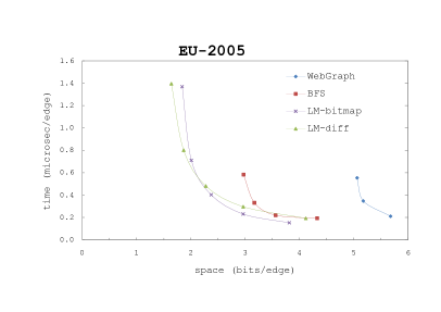
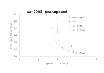
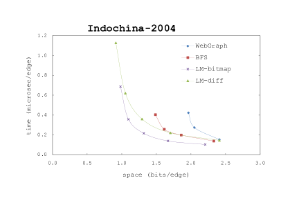
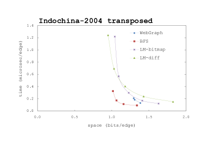
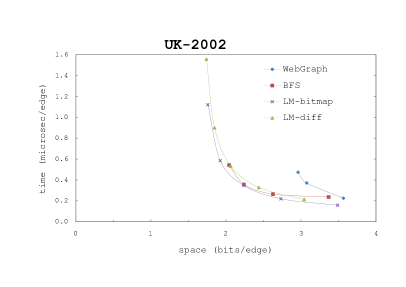
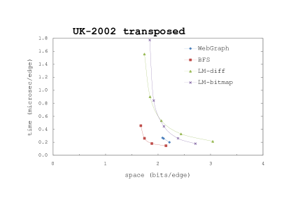
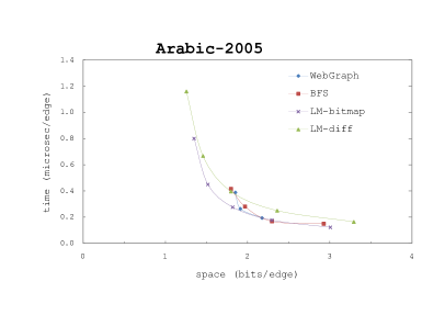
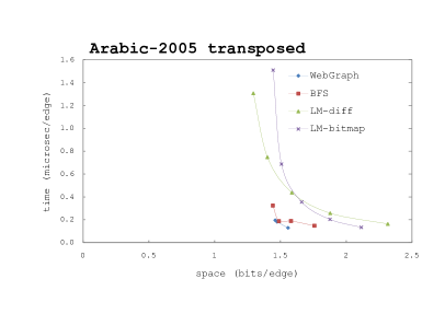
Figure 1: Compression ratios (bpe) and access times per edge

5.2 Varying the block size in the algorithm based on similarity of successive lists

Obviously, the block size should seriously affect the overall space used by the structure and the access time. Larger blocks mean that the Deflate algorithm is more successful in finding longer matches and the overhead from encoding first lines in a block without any reference is smaller. On the other hand, more lines have to be usually decoded before extracting the queried adjacency list.

In this experiment we run the 2a algorithm (the same implementation in Java) with each block of residuals terminated (and later Deflate-compressed) after reaching BSIZE of 1024, 2048, 4096, 8192 and 16384 bytes, respectively. The test computer had an Intel Pentium4 HT 3.0 GHz CPU, 1 GB of RAM, and was running Microsoft Windows XP Home SP3 (32-bit). The results (Table 5) show that doubling the block size implies space reduction by about 10% while the access time grows less than twice (in particular, using 8K blocks is only 2.0–2.5 times slower than using 2K blocks). Still, as the block size gets larger (compare the last two rows in the table), the improvement in compression starts to drop while the slowdown grows. For a reference, the access times of a practical Boldi–Vigna variant, BV (7,3), are 0.47 $\mu$s and 0.42 $\mu$s on the test machine.

	EU-2005		Indochina-2004
	bpe	time [$\mu$s]	bpe	time [$\mu$s]
1024	3.398	6.50	1.485	8.99
2048	2.869	8.91	1.292	12.05
4096	2.513	15.93	1.172	17.87
8192	2.286	27.60	1.101	29.83
16384	2.129	48.77	1.061	57.39

Table 5: Compression ratios and access times in function of the block size. 2a variant used. Tests run on the non-transposed graphs.

6 Conclusions

We presented two algorithms for Web graph compression, encoding blocks consisting of whole lines. All those algorithms achieve much better compression results than those presented in the literature, although two of them for the price of relatively slow access time. The more interesting algorithm, based on list merging, seems to be rather competitive to the algorithms known from the literature. Our approach lets achieve compression ratios not reported in the literature (LM-diff, 128), for one-directional queries, for moderate slow-down in list accesses (the best tradeoff here, however seem to be the variants LM-diff and LM-bitmap for $h=32$).

If even better compression ratios are welcome, then our SSL 4b variant can be considered, being more than an order of magnitude slower. We point out that one extreme tradeoff in succinct in-memory data structures is when accessing the structure is only slightly faster than reading data from disk. The niche for such a solution is when the given Web crawl cannot fit in RAM memory using less tight compressed representation and the stronger compression is already enough. The disk transfer rate is of relatively small imporantance here and what matters is the access time, which is about 10 ms or more for commodity 7200 RPM hard disks. Our algorithms spend significantly less time for extracting an average adjacency list, even if they are 1 or 2 orders of magnitude slower than the solutions from [7, 11, 12]. Another challenge is to compete with SSD disks which are not much faster than conventional disks in reading or writing sequential data but their access times are two orders of magniture smaller. Here our LM variants are fast enough, though.

Our algorithm works locally. In the future we are going to try to squeeze out some global redundancy while compressing the LM byproducts. A natural candidate for such experiments is the RePair algorithm [23, 13]. Other lines of research we are planning to follow are Web graph compression with bidirectional navigation and efficient compression of URLs. As for bidirectional navigation, the very recent idea from Claude and Ladra [10] is a prospective approach, in combination with LM, but even summing up naively the sizes of the two structures we build now, for the direct and the transposed graph, gives quite interesting results (see [19, 10] for comparison).

Appendix

	direct graph		transposed graph
	bpe	time [$\mu$s]	bpe	time [$\mu$s]
BV (7,3)	5.679	0.211	3.304	0.160
BFS, l4	4.325	0.192	3.367	0.144
BFS, l8	3.561	0.219	2.996	0.183
BFS, l16	3.169	0.330	2.803	0.289
BFS, l32	2.969	0.583	2.708	0.576
BFS, l1024	2.776	14.579	2.631	13.134
LM-bitmap, 8	3.814	0.152	2.951	0.173
LM-bitmap, 16	2.963	0.231	2.576	0.275
LM-bitmap, 32	2.373	0.403	2.233	0.508
LM-bitmap, 64	2.008	0.711	2.016	1.004
LM-bitmap, 128	1.838	1.370	1.963	2.176
LM-diff, 8	4.115	0.193	3.204	0.200
LM-diff, 16	2.964	0.296	2.543	0.329
LM-diff, 32	2.275	0.481	2.107	0.547
LM-diff, 64	1.867	0.802	1.854	0.931
LM-diff, 128	1.640	1.396	1.727	1.609

Table 6: EU-2005 dataset. Compression ratios (bpe) and access times per edge. All compressors are written in Java and were run with JRE 7. The extra data required to access the graph in random order are included.

	direct graph		transposed graph
	bpe	time [$\mu$s]	bpe	time [$\mu$s]
BV (7,3)	2.411	0.153	1.384	0.130
BFS, l4	2.331	0.137	1.339	0.091
BFS, l8	1.860	0.199	1.158	0.112
BFS, l16	1.615	0.257	1.063	0.173
BFS, l32	1.488	0.403	1.016	0.326
BFS, l1024	1.363	9.516	0.976	6.128
LM-bitmap, 8	2.207	0.103	1.630	0.121
LM-bitmap, 16	1.668	0.139	1.411	0.169
LM-bitmap, 32	1.320	0.216	1.228	0.297
LM-bitmap, 64	1.097	0.357	1.093	0.568
LM-bitmap, 128	0.982	0.687	1.040	1.219
LM-diff, 8	2.412	0.145	1.824	0.151
LM-diff, 16	1.704	0.221	1.428	0.239
LM-diff, 32	1.295	0.360	1.180	0.404
LM-diff, 64	1.053	0.620	1.030	0.694
LM-diff, 128	0.915	1.127	0.950	1.243

Table 7: Indochina-2004 dataset. Compression ratios (bpe) and access times per edge. All compressors are written in Java and were run with JRE 7. The extra data required to access the graph in random order are included.

	direct graph		transposed graph
	bpe	time [$\mu$s]	bpe	time [$\mu$s]
BV (7, 3)	3.567	0.225	2.218	0.200
BFS, l4	3.369	0.236	2.152	0.147
BFS, l8	2.627	0.264	1.883	0.181
BFS, l16	2.242	0.357	1.742	0.260
BFS, l32	2.042	0.542	1.673	0.455
BFS, l1024	1.851	12.618	1.621	10.370
LM-bitmap, 8	3.490	0.158	2.714	0.178
LM-bitmap, 16	2.733	0.219	2.381	0.260
LM-bitmap, 32	2.241	0.346	2.113	0.444
LM-bitmap, 64	1.925	0.584	1.919	0.841
LM-bitmap, 128	1.760	1.120	1.842	1.773
LM-diff, 8	3.853	0.201	3.043	0.213
LM-diff, 16	2.813	0.297	2.438	0.328
LM-diff, 32	2.203	0.468	2.064	0.532
LM-diff, 64	1.843	0.771	1.849	0.900
LM-diff, 128	1.632	1.336	1.742	1.557

Table 8: UK-2002 dataset. Compression ratios (bpe) and access times per edge. All compressors are written in Java and were run with JRE 7. The extra data required to access the graph in random order are included.

	direct graph		transposed graph
	bpe	time [$\mu$s]	bpe	time [$\mu$s]
BV (7, 3)	2.177	0.193	1.558	0.129
BFS, l4	2.927	0.150	1.759	0.147
BFS, l8	2.297	0.168	1.581	0.189
BFS, l16	1.970	0.280	1.488	0.188
BFS, l32	1.800	0.416	1.443	0.324
BFS, l1024	1.631	12.327	1.408	8.692
LM-bitmap, 8	3.008	0.122	2.116	0.133
LM-bitmap, 16	2.295	0.177	1.877	0.203
LM-bitmap, 32	1.820	0.276	1.662	0.355
LM-bitmap, 64	1.518	0.449	1.508	0.687
LM-bitmap, 128	1.350	0.799	1.445	1.509
LM-diff, 8	3.293	0.164	2.317	0.163
LM-diff, 16	2.361	0.250	1.879	0.258
LM-diff, 32	1.798	0.396	1.587	0.438
LM-diff, 64	1.459	0.667	1.401	0.748
LM-diff, 128	1.256	1.159	1.294	1.307

Table 9: Arabic-2005 dataset. Compression ratios (bpe) and access times per edge. All compressors are written in Java and were run with JRE 7. The extra data required to access the graph in random order are included.

References

- [1] V. N. Anh and A. F. Moffat: Local modeling for webgraph compression, in DCC, J. A. Storer and M. W. Marcellin, eds., IEEE Computer Society, 2010, p. 519.
- [2] A. Apostolico and G. Drovandi: Graph compression by BFS. Algorithms, 2(3) 2009, pp. 1031–1044.
- [3] Y. Asano, Y. Miyawaki, and T. Nishizeki: Efficient compression of web graphs, in COCOON, X. Hu and J. Wang, eds., vol. 5092 of Lecture Notes in Computer Science, Springer, 2008, pp. 1–11.
- [4] K. Bharat, A. Z. Broder, M. R. Henzinger, P. Kumar, and S. Venkatasubramanian: The Connectivity Server: Fast access to linkage information on the Web. Computer Networks, 30(1–7) 1998, pp. 469–477.
- [5] P. Boldi, M. Rosa, M. Santini, and S. Vigna: Layered label propagation: a multiresolution coordinate-free ordering for compressing social networks, in WWW, S. Srinivasan, K. Ramamritham, A. Kumar, M. P. Ravindra, E. Bertino, and R. Kumar, eds., ACM, 2011, pp. 587–596.
- [6] P. Boldi, M. Santini, and S. Vigna: Permuting web and social graphs. Internet Mathematics, 2009, pp. 257–283.
- [7] P. Boldi and S. Vigna: The webgraph framework I: Compression techniques, in WWW, S. I. Feldman, M. Uretsky, M. Najork, and C. E. Wills, eds., ACM, 2004, pp. 595–602.
- [8] N. Brisaboa, S. Ladra, and G. Navarro: K2-trees for compact web graph representation, in Proc. 16th International Symposium on String Processing and Information Retrieval (SPIRE), LNCS 5721, Springer, 2009, pp. 18–30.
- [9] G. Buehrer and K. Chellapilla: A scalable pattern mining approach to web graph compression with communities, in WSDM, M. Najork, A. Z. Broder, and S. Chakrabarti, eds., ACM, 2008, pp. 95–106.
- [10] F. Claude and S. Ladra: Practical representations for web and social graphs, in Proc. ACM Conference on Information and Knowledge Management, ACM, 2011, To appear.
- [11] F. Claude and G. Navarro: Fast and compact Web graph representations, Tech. Rep. TR/DCC-2008-3, Department of Computer Science, University of Chile, April 2008.
- [12] F. Claude and G. Navarro: Extended compact web graph representations, in Algorithms and Applications, T. Elomaa, H. Mannila, and P. Orponen, eds., vol. 6060 of Lecture Notes in Computer Science, Springer, 2010, pp. 77–91.
- [13] F. Claude and G. Navarro: Fast and compact web graph representations. ACM Transactions on the Web (TWEB), 4(4) 2010.
- [14] J. S. Culpepper and A. Moffat: Enhanced byte codes with restricted prefix properties, in SPIRE, M. P. Consens and G. Navarro, eds., vol. 3772 of Lecture Notes in Computer Science, Springer, 2005, pp. 1–12.
- [15] R. F. Geary, N. Rahman, R. Raman, and V. Raman: A simple optimal representation for balanced parentheses, in Combinatorial Pattern Matching, 15th Annual Symposium, CPM 2004, Istanbul,Turkey, July 5-7, 2004, Proceedings, S. C. Sahinalp, S. Muthukrishnan, and U. Dogrusöz, eds., vol. 3109 of Lecture Notes in Computer Science, Springer–Verlag, 2004, pp. 159–172.
- [16] S. Grabowski and W. Bieniecki: Tight and simple Web graph compression, in Proc. Prague Stringology Conference, J. Holub and J. Žd’árek, eds., 2010, pp. 127–137.
- [17] : Merging adjacency lists for efficient Web graph compression, in Proc. International Conference on Man-Machine Interactions, Springer, 2011, To appear.
- [18] X. He, M.-Y. Kao, and H.-I. Lu: A fast general methodology for information-theoretically optimal encodings of graphs. SIAM J. Comput., 30(3) 2000, pp. 838–846.
- [19] C. Hernández and G. Navarro: Compression of web and social graphs supporting neighbor and community queries, in Proc. 5th ACM Workshop on Social Network Mining and Analysis (SNA-KDD), ACM, 2011, To appear.
- [20] G. Jacobson: Succinct Static Data Structures, PhD thesis, 1989.
- [21] S. Ladra: Algorithms and Compressed Data Structures for Information Retrieval, PhD thesis, 2011.
- [22] N. J. Larsson and A. Moffat: Off-line dictionary-based compression. Proceedings of the IEEE, 88(11) Nov. 2000, pp. 1722–1732.
- [23] N. J. Larsson and A. Moffat: Off-line dictionary-based compression. Proceedings of the IEEE, 88(11) 2000, pp. 1722–1732.
- [24] J. I. Munro and V. Raman: Succinct representation of balanced parentheses, static trees and planar graphs, in IEEE Symposium on Foundations of Computer Science (FOCS), 1997, pp. 118–126.
- [25] G. Navarro and V. Mäkinen: Compressed full-text indexes. ACM Computing Surveys, 39(1) 2007, p. article 2.
- [26] P. Procházka and J. Holub: New word-based adaptive dense compressors, in IWOCA, J. Fiala, J. Kratochvíl, and M. Miller, eds., vol. 5874 of Lecture Notes in Computer Science, Springer, 2009, pp. 420–431.
- [27] K. Randall, R. Stata, R. Wickremesinghe, and J. Wiener: The link database: Fast access to graphs of the Web, 2001.
- [28] G. Turán: On the succinct representation of graphs. Discrete Applied Math, 15(2) May 1984, pp. 604–618.