Testing the Copernican and Cosmological Principles in the local universe with galaxy surveys

Abstract:

Cosmological density fields are assumed to be translational and rotational invariant, avoiding any special point or direction, thus satisfying the Copernican Principle. A spatially inhomogeneous matter distribution can be compatible with the Copernican Principle but not with the stronger version of it, the Cosmological Principle which requires the additional hypothesis of spatial homogeneity. We establish criteria for testing that a given density field, in a finite sample at low redshifts, is statistically and/or spatially homogeneous. The basic question to be considered is whether a distribution is, at different spatial scales, self-averaging. This can be achieved by studying the probability density function of conditional fluctuations. We find that galaxy structures in the SDSS samples, the largest currently available, are spatially inhomogeneous but statistically homogeneous and isotropic up to $\sim 100$ Mpc/h. Evidences for the breaking of self-averaging are found up to the largest scales probed by the SDSS data. The comparison between the results obtained in volumes of different size allows us to unambiguously conclude that the lack of self-averaging is induced by finite-size effects due to long-range correlated fluctuations. We finally discuss the relevance of these results from the point of view of cosmological modeling.

1 Introduction

The attempts to construct cosmological models including spatial inhomogeneities have experienced a renewed interest in connection with the evidences for a speeding up expansion of the universe as shown by the supernovae observations [1, 2]. Indeed, the deduction of the existence of dark energy is based on the assumption that the universe has a Friedmann-Robertson-Walker (FRW) geometry. There have been various claims that these observations can at least in principle be accounted for without the presence of any dark energy, if we consider the possibility of inhomogeneities. This can happen in two different ways: locally via back-reaction [3, 4, 5] or by placing the observer in a special point of the local universe [6, 7]. Direct observational tests of the basic assumptions used in the derivation of the FRW models are thus of considerable importance. A widespread idea in cosmology is that the so-called concordance model of the universe combines two fundamental assumptions. The first is that the dynamics of space-time is determined by Einstein’s field equations. The second is that the universe is homogeneous and isotropic. This hypothesis, usually called the Cosmological Principle, is though to be a generalization of the Copernican Principle that “the Earth is not in a central, specially favored position” [8, 9]. The FRW model is derived under these two assumptions and it describes the geometry of the universe in terms of a single function, the scale factor, which obeys to the Friedmann equation [10]. There is a subtlety in the relation between the Copernican Principle (all observes are equivalent and there are no special points and directions) and the Cosmological Principle (the universe is homogeneous and isotropic). Indeed, the fact that the universe looks the same, at least in a statistical sense, in all directions and that all observers are alike does not imply spatial homogeneity of matter distribution. It is however this latter condition that allows us to treat, above a certain scale, the density field as a smooth function, a fundamental hypothesis used in the derivation of the FRW metric. Thus there are distributions which satisfy the Copernican Principle and which do not satisfy the Cosmological Principle [11]. These are statistically homogeneous and isotropic distributions which are also spatially inhomogeneous. Therefore the Cosmological Principle represents a specific case, holding for spatially homogeneous distributions, of the Copernican Principle which is, instead, much more general. Statistical and spatial homogeneity refer to two different properties of a given density field. The problem of whether a fluctuations field is compatible with the conditions of the absence of special points and direction can be reformulated in terms of the properties of the probability density functional (PDF) which generates the stochastic field. In what follows we precisely discuss this point, both from a theoretical and observational point of view.

Different strategies have been proposed to test the large scale isotropy of matter distribution and the basic predictions of homogeneous models [12]. (i) If the cosmic microwave background radiation (CMBR) is anisotropic around distant observers, Sunyaev-Zeldovich scattered photons have a distorted spectrum that reflects the spatial inhomogeneity [13, 14]. (ii) Tests, based on future supernovae surveys, to determine whether there is a geometric cusp at the origin [15, 6]. (iii) Geometric effects on distance measurements [16, 17]. (iv) There are then some indirect tests [18]. All these approaches thus consider mainly data from the CMBR and from supernovae surveys and they do not directly test for spatial homogeneity.

However Ellis [19] pointed out that ”Spatial homogeneity is one of the foundations of standard cosmology, so any chance to check those foundations observationally should be welcomed with open arms”. As recently it became possible to measure directly the nature of the spatial galaxy distribution by using galaxy redshift surveys, in this paper we present a new test focused to determine whether matter distribution is statistically homogeneous and isotropic and whether it is spatially homogeneous. Testing these two hypotheses can be achieved by characterizing galaxy distribution from the latest data of the Sloan Digital Sky Survey (SDSS) [20].

The paper is organized as follows. In Sect.2 we recall some basic statistical properties of spatially homogeneous and inhomogeneous distributions. Particularly we discuss that an inhomogeneous distribution can be fully compatible with the Copernican Principle that there are not special points or directions. The compatibility of a fluctuating density field, regardless of whether it is spatially homogeneous, is encoded in the properties of its PDF. This is a very fundamental issue which, in our opinion, has been overlooked in the literature. For example, in ref. [10] it is stated that ”The visible universe seems the same in all directions around us, at least if we look out to distances larger than about 300 million light years”, to mean that it is spatially homogeneous as then the standard FRW modeling is used to derive a number of properties. We point out instead that the fact that the observable galaxy distribution looks the same in all directions around us implies statistical homogeneity and not necessarily spatial homogeneity. This is the key point which requires a more detailed investigation from the point of view of theoretical modeling, as the lack of spatial homogeneities has a deep impact on it. For instance the works on back-reaction [3, 4, 5] consider precisely the effect statistically homogeneous large-amplitude fluctuations (i.e. spatial inhomogeneities) up to few hundreds Mpc on the geometrical properties of the large scale universe.

In Sect.3 we present two simple examples which may clarify this point further. Note that the discussion in Sects.2-3 refers to an ideal case of a distribution in an Euclidean space and does not consider the additional complication introduced by a curved and time dependent geometry. However this treatment is fully valid in the galaxy samples we consider, as they are limited to low redshifts, i.e. $z<0.2$. It is clear that any conclusion we can draw about the statistical properties of galaxy fluctuations is limited to the range of scales we considered.

We then pass, in Sect.4, to the discussion of the observed galaxy redshift samples provided by the data release 7 (DR7) of the Sloan Digital Sky Survey (SDSS). Our main result is that galaxy distribution as observed by current surveys is inhomogeneous but not characterized by any special point of direction, i.e. it is statistically homogeneous but spatially inhomogeneous. This fact, was overlooked in the past [21] when only the projection on the sky of the galaxy density field was available. Having three-dimensional maps allows us to test statistically homogeneity and isotropy from many points (observers), which was not possible for projection on the sky.

In Sect.5 we discuss the relevance of the results obtained in the low-redshift galaxy surveys which respect to the theoretical modeling and the extension to the test we introduced to higher redshift. Particularly we consider the fact that we make observations on our past light-cone which is not a space-like surface. Finally we draw our conclusions in Sect.6.

2 Ergodicity and self-averaging

Mass density fields can be represented as stationary stochastic processes. The stochastic process consists in extracting the value of the microscopic density function $\rho(\vec{r})$ at any point of the space. This is completely characterized by its probability density functional ${\cal P}[\rho(\vec{r})]$. This functional can be interpreted as the joint probability density function of the random variables ${\rho}(\vec{r})$ at every point $\vec{r}$. If the functional ${\cal P}[\rho(\vec{r})]$ is invariant under spatial translations then the stochastic process is statistically homogeneous or translational invariant (stationary) [11]. When ${\cal P}[\rho(\vec{r})]$ is also invariant under spatial rotation then the density field is statistically isotropic [11].

Matter distribution in cosmology then is considered to be a realization of a stationary stochastic point process. This is enough to satisfy the Copernican Principle i.e., that there are no special points or directions; however this does not imply spatial homogeneity. Spatially homogeneous stationary stochastic processes satisfy the special and stronger case of the Copernican Principle described by Cosmological Principle. Indeed, isotropy around each point together with the hypothesis that the matter distribution is a smooth function of position i.e., that this is analytical, implies spatial homogeneity. (A formal proof can be found in [22].) This is no longer the case for a non-analytic structure (i.e., not smooth), for which the obstacle to applying the FRW solutions has in fact solely to do with the lack of spatial homogeneity [23].

The condition of spatial homogeneity (uniformity) is satisfied if the ensemble average density of the field $\langle\rho\rangle$ is strictly positive. Otherwise, when $\langle\rho\rangle=0$ the distribution is inhomogeneous. We are interested in the finite sample properties of a given density field and for this reason we should introduce the concept of spatial average. First, we remind that a crucial assumption usually used is that stochastic fields are required to satisfy spatial ergodicity. Let us take a generic observable ${\cal F}={\cal F}(\rho(\vec{r}_{1}),\rho(\vec{r}_{2}),...)$ function of the mass distribution $\rho(\vec{r})$ at different points in space $\vec{r}_{1},\vec{r}_{2},...$. Ergodicity implies that $\left<{\cal F}\right>=\overline{{\cal F}}=\lim_{V\rightarrow\infty}\overline{{\cal F}}_{V}$, where $\overline{{\cal F}}_{V}$ is the spatial average in a finite volume $V$ [11]. When considering a finite sample realization of a stochastic process, and thus statistical estimators of asymptotic quantities, the first question to be sorted out concerns whether a certain observable is self-averaging in a given finite volume [24, 25]. In general a stochastic variable $\cal{F}$ is self-averaging if ${\cal F}=\left<{\cal F}\right>$ (see [25] for a more detailed discussion). Thus if this is ergodic, $\overline{{\cal F}}=\left<{\cal F}\right>$, then it is also self-averaging as $\overline{{\cal F}}=\left<\overline{{\cal F}}\right>$: finite sample spatial averages must be self-averaging in order to satisfy spatial ergodicity.

A simple test to determine whether a distribution is stationary and self-averaging in a given sample of linear size $L$ consists in studying the probability density function (PDF) of conditional fluctuations ${\cal G}$ (which contains, in principle, all information about moments of any order) in sub-samples of linear size $L^{\prime}<L$ placed in different and non-overlapping spatial regions of the sample (i.e., $S_{1},S_{2},...S_{N}$). That the self-averaging property holds is shown by the fact that $P({\cal G},L^{\prime};S_{i})$ is the same, modulo statistical fluctuations, in the different sub-samples, i.e., $P({\cal G},L^{\prime};S_{i})\approx P({\cal G},L^{\prime};S_{j})\;\forall i\neq j.$ On the other hand, if determinations of $P({\cal G},L^{\prime};S_{i})$ in different sample regions $S_{i}$ show systematic differences, then there are two different possibilities: (i) the lack of the property of stationarity or (ii) the breaking of the property of self-averaging due to a finite-size effect related to the presence of long-range correlated fluctuations. Therefore while the breaking of statistical homogeneity and/or isotropy imply the lack of self-averaging property the reverse is not true. However, if the determinations of the spatial averages give sample-dependent results, this implies that those statistical quantities do not represent the asymptotic properties of the given distribution [25].

To test statistical and spatial homogeneity it is necessary to employ statistical quantities that do not require the assumption of spatial homogeneity inside the sample and thus avoid the normalization of fluctuations to the estimation of the sample average [25]. These are conditional quantities, which describe local properties of the distribution. For instance, we consider the number of points $N_{i}(r)$ contained in a sphere of radius $r$ centered on the $i^{th}$ point. This depends on the scale $r$ and on the spatial position of the $i^{th}$ sphere’s center, namely its radial distance $R_{i}$ from a given origin and its angular coordinates $\vec{\alpha}_{i}$. Integrating over $\vec{\alpha}_{i}$ for fixed radial distance $R_{i}$, we obtain that $N_{i}(r)=N(r;R_{i})$ [25].

3 Breaking of self-averaging properties

In order to illustrate an example let us consider a case where translation invariance is broken. We generate a Poisson-Radial distribution (PRD) which is a inhomogeneous distribution that can mimic the effect of a “local hole” around the origin. In a sphere of radius $R_{0}=1$ we place, for instance, $N=2\cdot 10^{5}$ points. In each bin at radial distance from the sphere center $[R_{i},R_{i+1}]$, and with thickness $\Delta R$, the distribution is Poissonian with a density varying as $n(R)=n_{0}\cdot R\;,$ where $n_{0}$ is a constant. We determine the PDF $P(N;r)$ of conditional fluctuations obtained by making an histogram of the values of $N(r;R)$ at fixed $r$ (see the upper panels of Fig.1). The whole-sample PDF is clearly left-skewed: this occurs because the peak of the PDF corresponds to the most frequent counts which are at large radial distance simply because shells far-way from the origin contain more points. The spread of the PDF can easily be related to the difference in the density between small and large radial distances in the sample. By computing the PDF into two non-overlapping sub-samples, nearby to and faraway from the origin, one may clearly identify the systematic dependence of this quantity on the specific region where this is measured. This breaking of the self-averaging properties is caused by the radial-distance dependence of the density and thus by the breaking of translational invariance.

Let us now consider a stationary stochastic distribution, where the breaking self-averaging properties is due to the effect of large scale fluctuations. An example is represented by the inhomogeneous toy model (ITM) constructed as follows. We generate a stochastic point distribution by randomly placing, in a two-dimensional box of side $L$, structures represented by rectangular sticks. We first distribute randomly $N_{s}$ points which are the sticks centers: they are characterized by a mean distance $\Lambda\approx(L^{3}/N_{s})^{1/3}$. Then the orientation of each stick is chosen randomly. The points belonging to each stick are also placed randomly within the stick area, that for simplicity we take to be $\ell\times\ell/10$. The length-scale $\ell$ can vary, for example being extracted from a given PDF. The number of sticks placed in the box fixes $\Lambda$. This distribution is by construction stationary i.e., there are no special points or directions. When $\ell\geq L$ and $\Lambda\leq L$ but with $\ell$ varying in such a way that there can been large differences in its size, the resulting distribution is long-range correlated, spatially inhomogeneous and it can be not self-averaging. This latter case occurs when, by measuring the PDF of conditional fluctuations in different regions of a given sample, one finds, for large enough $r$, systematic differences in the PDF shape and peak location (see the bottom panels Fig.1). These are due to the strong correlations extending well over the size of the sample.

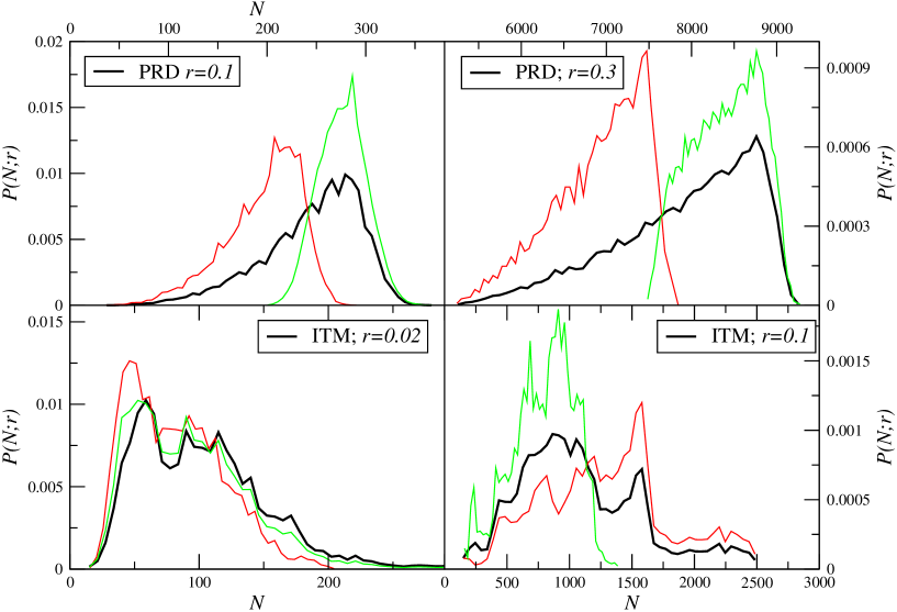
Figure 1: Upper panels: The PDF for $r=0.1$ (left) and $r=0.3$ (right) for PRD computed for the whole sample (black line). The red (green) line shows the PDF measured in the sub-sample placed closer to (father from) the origin. Lower Panels: The same for the ITM at scales $r=0.02$ (left) and $r=0.1$ (right)

How can we distinguish between the case in which a distribution is not self-averaging because it is not statistically translational invariant and when instead this is stationary but fluctuations are too extended in space and have too large amplitude ? The clearest test is to change the scale $r$ where $P(N,r)$ is measured, and determining whether the PDF is self-averaging. Indeed, in the case of the PRD the strongest differences between the PDF measured in regions placed at small and large radial distance from the structure center, occur for small $r$. This is because the local density has the largest variations at small and large radial distances by construction. When $r$ grows, different radial scales are mixed as the generic sphere of radius $r$ pick up contributions both from points nearby the origin and from those far away from it, resulting in a smoothing of local differences. Instead, in the ITM for small $r$ the difference is negligible while for large enough $r$ the different determinations of the local density start to feel the presence of a few large structures which dominate the large scale distribution in the sample.

4 Galaxy Catalogs

Let us now consider two (volume limited [25]) samples constructed from the data release 6 (DR6) and DR7 [20] of the SDSS (see [25, 26] for details). We cut each sample volume into two regions, one nearby us (small $R$  ) and the other faraway from us (large $R$). We determine the PDF $P(N;r)$ separately in both regions, and at two different $r$ scales. In a first case (left panels of Fig.2), at small scales ($r=10$ Mpc/h), the distribution is self-averaging both in the DR6 sample (that covers a solid angle $\Omega_{DR6}=0.94$ sr.) than in the sample extracted from DR7 ($\Omega_{DR7}=1.85$ sr. $\approx 2\times\Omega_{DR6}$ sr). Indeed, the PDF is statistically the same in the two sub-samples considered. Instead, for larger sphere radii i.e., $r=80$ Mpc/h, (right panels of Fig.2) in the DR6 sample, the two PDF show clearly a systematic difference. Not only the peaks do not coincide, but the overall shape of the PDF is not smooth and different. On the other hand, for the sample extracted from DR7, the two determinations of the PDF are in very good agreement. We conclude therefore that, in DR6 for $r=80$ Mpc/h there are large density fluctuations which are not self-averaging because of the limited sample volume [25]. They are instead self-averaging in DR7 because the volume is increased by a factor two.

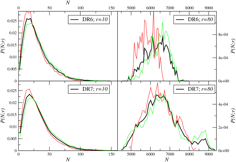
Figure 2: PDF of conditional fluctuations in the sample defined by $R\in[125,400]$ Mpc/h and $M\in[-20.5,-22.2]$ in the DR6 (upper panels) and DR7 (lower panels) data, for two different values of the sphere radii $r=10$ Mpc/h and $r=80$ Mpc/h. In each panel, the black line represents the full-sample PDF, the red line (green) the PDF measured in the half of the sample closer to (farther from) the origin.

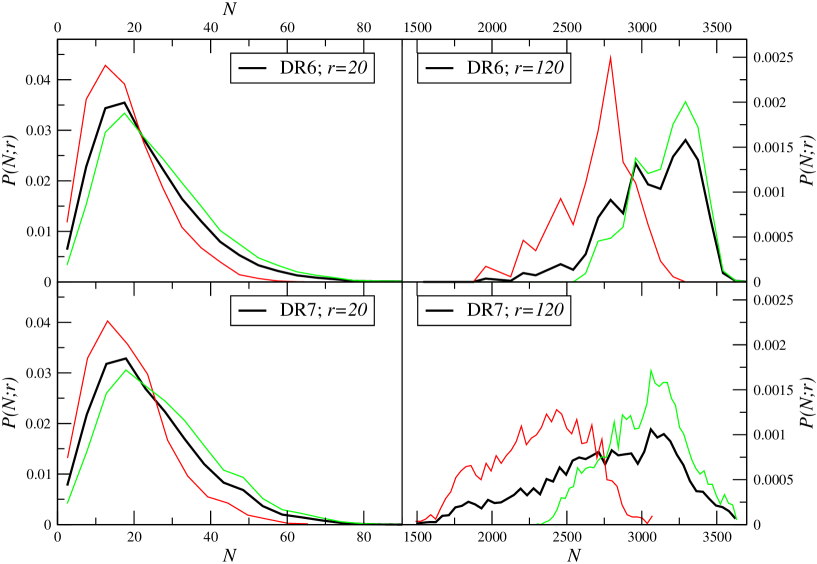
Figure 3: The same of Fig.2 but for the sample defined by $R\in[200,600]$ Mpc/h and $M\in[-21.6,-22.8]$ and for $r=20,120$ Mpc/h.

The lack of self-averaging properties at large scales in the DR6 sample is due to the presence of large scale galaxy structures which correspond to density fluctuations of large amplitude and large spatial extension, whose size is limited only by the sample boundaries. The appearance of self-averaging properties in the larger DR7 sample volumes is the unambiguous proof that the lack of them is induced by finite-size effects due to long-range correlated fluctuations.

For the deepest sample we consider, which include mainly bright galaxies, the breaking of self-averaging properties does not occur as well for small $r$ but it is found for large $r$. This can be due to the same effects i.e., that the sample volumes are still too small as even in DR7 for $r=120$ Mpc/h we do not detect self-averaging properties (right panels of Fig.3). Other radial distance-dependent selections, like galaxy evolution [27], could in principle give an effect in the same direction. However this would not affect the conclusion that, on large enough scales, self-averaging is broken. Note that, contrary to the PRD case, in the SDSS samples for small values of $r$ the PDF is found to be statistically stable in different sub-regions of a given sample. For this reason we do not interpret the lack of self-averaging properties as due to a “local hole” around us. As discussed above, this would affect all samples and all scales, which is indeed not the case. Because of these large fluctuations in the galaxy density field, self-averaging properties are well-defined only in a limited range of scales. Only in that range it will be statistically meaningful to measure whole-sample average quantities [25, 26].

5 Discussion

The discussion in the previous sections was meant to treat the statistical properties of the galaxy density field in a spatial hyper-surface. As mentioned above, this is an approximation valid when considering the galaxy distribution limited to relatively low redshifts, i.e. $z<0.2$. In particular, we have developed a test to focus on the properties of statistical and homogeneity homogeneity in nearby redshift surveys. The assumptions of the cosmological model enter in the data analysis when calculating the metric distance from the redshift and the absolute magnitude from the apparent one and the redshift. However, given that second order corrections are small for $z<0.2$, our results are basically independent on the chosen underlying model to reconstruct metric distances and absolute magnitudes from direct observables. In practice we can use just a linear dependence of the metric distance on the redshift (which is, to a very good approximation, compatible with observations at low redshift). For this same reason we can approximate the observed galaxies as lying in a spatial hyper-surface.

In the ideal case of having a very deep survey, up to $z\approx 1$, we should consider that we make observations on our past light-cone which is not a space-like surface. In order to evolve our observations onto a spatial surface we would need a cosmological model, which at such high redshift can play an important role in the whole determination of statistical quantities. A sensible question is whether we can to reformulate the statistical test given so that it can be applied to data on our past light-cone, and not on an assumed spatial hyper-surface. Going to higher redshift poses a number of question, first of the all the one of checking the effect of the assumptions used to construct metric distances and absolute magnitudes from direct observables. Testing these effects can be simply achieved by using different distance-redshift relations.

However, we note that a smooth change of the distance-redshift relation as implied by a given cosmological model, may change the average behavior of the conditional density as a function of redshift but it cannot smooth out fluctuations, i.e. it cannot substantially change the PDF of conditional fluctuations when they are measured locally. Indeed, our test is based on the characterization of the PDF of conditional fluctuations and not only of the behavior of the conditional average density as a function of distance. The PDF provides, in principle, with a complete characterization of the fluctuations statistical properties. We have shown that the PDF of fluctuations has a clear imprint when the distribution is spherically symmetric or when it is spatially inhomogeneous but statistically homogeneous.

The fact that we analyze conditional fluctuations means that we consider only local properties of the fluctuations: local with respect to an observer placed at different radial (metric) distances from the us, i.e. at different redshifts. For the determination of the PDF we have to consider two different length scale: the first is the (average) metric distance $R$ of the galaxies on which we center the sphere and the second is the sphere radius $r$. Irrespective of the value of $R$ when $r$ is smaller than a few hundreds Mpc (i.e., when its size is much smaller than any cosmological length scale), we can always locally neglect the specific $R(z)$ relation induced by a specific cosmology. In other words, when the sphere radius is limited to a few hundreds Mpc we can approximate the measurements of the conditional density to be performed on a spatial hyper-surface.

The whole description of the matter density field in terms of FRW or even Lemaitre-Tolman-Bondi (LTB) cosmologies, refer to the behavior of, for instance, the average matter density as a function of time (in the LTB case also as a function of scale) but it says anything on the fluctuation properties of the density field. Thus, when looking at different epochs in the evolution of the universe, we should detect that the average density varies (being higher in early epochs). This means only that the peak of the PDF will be located at different $N$ values, but the shape of the PDF is unchanged by this overall (smooth) evolution. Fluctuations are simply not present in the FRW or LTB models, and the whole issue of back-reaction studies is to understand what is their effect.

Note that models which explain dark energy through inhomogeneity do so using a spatial under-density in the matter density which varies on Gpc scales — out to $z\approx 1$ [6]. These models by placing us at the center of the universe, violate the Copernican Principle. In this respect we note that, while we cannot make any claim for $z>0.2$ based on current data, the fact that galaxy distribution is spatially inhomogeneous but statistically homogeneous up to 100 Mpc/h, already poses intriguing theoretical problems. Indeed, in that in that range of scales, the modeling of the matter density field as a perfect fluid, as required by the FRW models, is not even a rough approximation. As pointed out by various authors [28, 29], if the linearity of the Hubble law is a consequence of spatial homogeneity, how is it that observations show that it is very well linear at the same scales where matter distribution is inhomogeneous ? Recently [17] it was speculated a solution to this apparent paradox can be found by considering both the effects of back-reaction and the synchronization of clocks. While this is certainly an interesting approach, the formulation of a more complete and detailed theoretical framework is still lacking.

Finally we note that there are several complications in radially inhomogeneous models at high redshift. Beyond the change of the distance-redshift relation, discussed above, another is how structure evolves from our past light-cone onto a surface of constant time. Thus in order to make a precise test on the spatial properties of a given model, one needs to develop the corresponding theory of structure formation. However, at least at low redshifts, it seems implausible that the main feature of the model, the specific redshift-dependence of the spatial density, will not be the clearer prediction for the observations of galaxy structures.

6 Conclusions

We have presented tests on both the Copernican and Cosmological Principles at low redshift, where we can neglect the important complications of evolving observations onto a spatial surface for which we need a specific cosmological model. We have discussed however that the statistical properties of the matter density field up to a few hundreds Mpc is crucially important for the theoretical modeling.

We have discussed that these are achieved by considering the properties of the probability density function of conditional fluctuations in the available galaxy samples. We have shown that galaxy distribution in different samples of the SDSS is compatible with the assumptions that this is transitionally invariant, i.e. it satisfies the requirement of the Copernican Principle that there are no spacial points or directions. On the other hand, we found that there are no clear evidences of spatial homogeneity up to scales of the order of the samples sizes, i.e. $\sim 100$ Mpc/h . This implies that galaxy distribution is not compatible with the stronger assumption of spatial homogeneity, encoded in the Cosmological Principle. In addition, at the largest scales probed by these samples (i.e., $r\approx 120$ Mpc/h) we found evidences for the breaking of self-averaging properties, i.e. that the distribution is not statistically homogeneous. Forthcoming redshift surveys will allow us to clarify whether on such large scales galaxy distribution is still inhomogeneous but statistically stationary, or whether the evidences for the breaking of spatial translational invariance found in the SDSS samples were due to selection effects in the data.

- [1] Riess, A. G., et al., Astron. J. 116 (1998) 1009
- [2] Perlmutter, S. et al., Astrophys. J. 517 (1999) 565
- [3] Buchert, T. Gen. Rel. Grav. 32 (2000) 105
- [4] Wiltshire, D.L., Phys. Rev. Lett. 99 (2007) 251101
- [5] Räsänen, S., J. Cosm. Astr. Phys. 11 (2006) 003
- [6] Clifton T., Ferreira, P. G., Land, K. Phys. Rev. Lett. 101 (2008) 131302
- [7] Célérier M.N., New Advan. Phys. 1 (2007) 29
- [8] Bondi, H. Cosmology, (Cambridge University Press, Cambridge, 1952).
- [9] Clifton T., Ferreira, P. G., Phys. Rev. D 80 (2009) 103503
- [10] Weinberg, S., Cosmology (Oxford University Press, Oxford, 2008)
- [11] Gabrielli A., Sylos Labini F., Joyce M., Pietronero L., Statistical Physics for Cosmic Structures (Springer Verlag, Berlin, 2005)
- [12] Ellis, G.F.R, 2008, in the proc. of the Conference “Dark Energy and Dark Matter”
- [13] Goodman, J., Phys. Rev. D 52 (1995) 1821
- [14] Caldwell R., Stebbins, A., Phys. Rev. Lett. 100 (2008) 191302
- [15] Vanderveld, R.A., et al., Phys. Rev. D 74 (023506) 2006
- [16] Clarkson, C., Bassett, B.A., Lu T.C., Phys. Rev. Lett. 101 (2008) 011301
- [17] Wiltshire, D.L., Phys. Rev. D 80 (2009) 123512
- [18] Lima, L. M., Vitenti S., Reboucas, M.J., Phys. Rev. D 77 (2008) 083518
- [19] Ellis, G., Nature 452 (2008) 158
- [20] Adelman-McCarthy, J.K., et al., Astrophys. J. Suppl. 175 (2008) 297
- [21] Peebles, P.J.E., Principles Of Physical Cosmology, (Princeton University Press, Princeton, New Jersey, 1993)
- [22] Straumann, N., Helv. Phys. Acta 47 (197) 379
- [23] Joyce, M., et al., Europhys. Lett. 50 (2000) 416
- [24] Aharony, A., Harris, B., Phys. Rev. Lett. 77 (1996) 3700
- [25] Sylos Labini, F. Vasilyev, N.L., Baryshev, Y.V., Astron. Astrophys. 508 (2009) 17
- [26] Antal, T., Sylos Labini, F., Vasilyev, N.L., Baryshev, Yu. V., Europhys. Lett. 88 (2009) 59001
- [27] Loveday, J., Mon. Not. R. Acad. Soc 347 (2004) 601
- [28] Sylos Labini F., Montuori, M. Pietronero, L. Phys. Rept. 293 (1998) 61
- [29] Wiltshire, D.L., Int. J. Mod. Phys. D 17 (2008) 641
- [30] Vasilyev, N.L., Baryshev, Yu. V., Sylos Labini, F., Astron. Astrophys. 447 (2006) 431
- [31] Sylos Labini, F., Vasilyev, N.L., Baryshev, Yu. V., Europhys. Lett. 85 (2009) 29002
- [32] Sylos Labini, F., Vasilyev, N.L., Baryshev, Yu. V., Astron. Astrophys. 496 (2009) 7