Developing Homogeneous Isotropic Turbulence

Abstract

We investigate the self-similar evolution of the transient energy spectrum which precedes the establishment of the Kolmogorov spectrum in homogeneous isotropic turbulence in three dimensions using the EDQNM closure model. The transient evolution exhibits self-similarity of the second kind and has a non-trivial dynamical scaling exponent which results in the transient spectrum having a scaling which is steeper than the Kolmogorov $k^{-5/3}$ spectrum. Attempts to detect a similar phenomenon in DNS data are inconclusive owing to the limited range of scales available.

I Introduction to transient spectra in turbulence

Although a large amount of work has been done characterising the properties of the Kolmogorov $k^{-5/3}$ spectrum of three dimensional turbulence, rather less attention has been paid to the transient evolution which leads to its establishment. This transient evolution is essentially non-dissipative since it describes the cascade process before it reaches the dissipation scale. Part of the reason why this process has attracted relatively little attention is that this transient evolution is very fast, typically taking place within a single large eddy turnover time. It is thus of little relevance to the developed turbulence regime of interest in many applications. Nevertheless, one may ask whether this developing turbulence, as one might call this transient regime, displays any interesting scaling properties. Previous studies of the developing regime in weak magnetohydrodynamic (MHD) turbulence Galtier et al. (2000) suggest that this transient regime might have non-trivial scaling properties: in this case it was found that the establishment of the Kolmogorov spectrum is preceded by a transient spectrum which is steeper than the Kolmogorov spectrum. This latter is, in turn, set up from right to left in wavenumber space only after the transient spectrum has reached the end of the inertial range and started to produce dissipation.

Subsequent studies suggest that this behaviour, in particular the occurence of a non-trivial dynamical scaling exponent, is typical for turbulent cascades which are finite capacity - meaning that the stationary spectrum can only contain a finite amount of energy. The Kolmogorov spectrum of three dimensional turbulence is in the class of finite capacity systems, as we shall see below. There are, however, examples of other turbulent cascades which are not - infinite capacity cascades are common in wave turbulence for example Newell et al. (2001). In addition to the MHD cascade mentioned above, examples of non-trivial scaling exponents in finite capacity cascades have been found in developing wave turbulence Connaughton et al. (2003); Connaughton and Newell (2010), Bose-Einstein condensation Lacaze et al. (2001); Connaughton and Pomeau (2004) and cluster-cluster aggregation Lee (2001). Although a possible heuristic explanation of the transient scaling in the MHD context has been put forward in Galtier et al. (2005), this heuristic relies heavily on the anisotropy of the MHD cascade and does not seem readily generalisable to other contexts. In general, the transient exponent is associated with a self-similarity problem of the second kind Barenblatt (1996). From a mathematical point of view, its solution requires solving a nonlinear equation in which the exponent appears as a parameter which is fixed by requiring consistency with boundary conditions. It is probably unrealistic to expect that there is a general heuristic argument capable of resolving such a mathematically challenging problem. This is not to say, however, that particular cases may not be amenable to heuristic arguments which take into account the underlying physical mechanisms driving the transient evolution rather than taking a purely mathematical point of view.

This issue has not yet been studied in the context of homogeneous isotropic turbulence. Investigations of transient spectra in the classical Leith closure model Leith (1967) have suggested, however, that the transient spectrum of developing homogeneous isotropic turbulence is indeed non-trivially steeper than $k^{-5/3}$ Connaughton and Nazarenko (2004). In this work, we investigate the transient evolution of homogeneous isotropic turbulence using the Eddy-Damped Quasi-Normal Markovian (EDQNM) closure model and direct numerical simulation (DNS) of the Navier-Stokes equation.

The transient spectrum might be expected to evolve self-similarly. In other words there is a typical wavenumber, $s(t)$, which grows in time, and a dynamical scaling exponent, $a$, such that

$$E_{k}(t)\asymp c\,s(t)^{a}\,F(\xi)\hskip 28.45274pt\mbox{where $\xi=\frac{k}{s(t)}$.}$$ (1)

Here $\asymp$ denotes the scaling limit: $k\to\infty$, $s(t)\to\infty$ with $\xi$ fixed and $c$ is an order unity constant which ensures that $E_{k}(t)$ has the correct physical dimensions, ${\mathrm{L}}^{3}\,{\mathrm{T}}^{-2}$. As we shall see, if the exponent, $(5+a)/2$, is greater than 1, then the characteristic wavenumber diverges in finite time corresponding to a cascade which accelerates “explosively”. The direct cascade in 3D turbulence is of this type. The characteristic wavenumber is most easily defined as a ratio of moments of the energy spectrum. Let us define

$$M_{n}(t)=\int_{0}^{\infty}k^{n}\,E_{k}(t)\,dk.$$ (2)

Eq. (1) suggests that the ratio $M_{n+1}(t)/M_{n}(t)$ is proportional to $s(t)$ so that we may define a typical scale intrinsically by

$$s_{n}(t)=\frac{M_{n+1}(t)}{M_{n}(t)}.$$ (3)

A little caution is required: we must take $n$ sufficiently high to ensure that the moments $M_{n}(t)$ used in defining the typical scale, converge at zero. Otherwise, the integral is dominated by the initial condition or forcing scale and does not capture the scaling behaviour. In this paper, we mostly take $n=2$, which turns out to be sufficient for our purposes, although we will compare the behaviour obtained for $n=2$ and $n=3$ in our numerical simulations to assure the reader that the picture is consistent.

We would like to emphasise that the self-similar transient dynamics which we study in this paper occur before the onset of dissipation. This is in contrast to the transient dynamics describing the long time decay of homogeneous isotropic turbulence after the onset of dissipation which are also believed to exhibit self-similarity. See Lavoie et al. (2007) for recent experiments and a review of previous work. Some numerical results on the long time transient dynamics of the EDQNM model can be found in Lesieur et al. (2005). The pre-dissipation transient occurs very quickly. Indeed, as we shall see, the typical scale, $s(t)$, in this regime diverges as $s(t)\sim(t^{*}-t)^{b}$ where $t^{*}$ is the time at which the onset of dissipation occurs (typically less than a single turnover time) and $b<0$. For finite Reynolds number, this singularity is regularised by the finiteness of the dissipation scale. The fact that, in the limit of infinite Reynolds number, the typical scale can grow by an arbitrary amount in an arbitrarily small time interval as $t^{*}$ is approached explains the statement often found in the literature that the Kolmogorov spectrum is established quasi-instantaneously in the limit of large Reynolds number.

II The EDQNM model

In this section we examine the self-similar solutions of the EDQNM model Orszag (1970). The structure of the EDQNM model can be obtained in different ways. One way is starting from the Quasi-Normal assumption Monin and Yaglom (1975). Another way is by simplifying the Direct Interaction Approximation Kraichnan (1959) which was obtained by applying a renormalized perturbation procedure to the Navier-Stokes equation. It is thus directly related to the Navier-Stokes equation, unlike the Leith model which was heuristically proposed to capture some features of the nonlinear transfer in isotropic turbulence. However, recent work Clark et al. (2010) showed that the structure of the Leith model can be obtained by retaining a subset of triad interactions involving elongated triads from closures like EDQNM. Since EDQNM contains a wider variety of triad interactions, it is able to capture more details of the actual dynamics of Navier-Stokes turbulence, as for example illustrated in Bos and Bertoglio (2006). At the same time it has the advantage over DNS that much higher Reynolds numbers can be obtained.

The EDQNM model closes the Lin-equation by expressing the nonlinear triple correlations as a function of the energy spectrum,

$$\frac{\partial E_{k}}{\partial t}=\mathrm{T}\left[E_{k}\right]-2\,\nu\,k^{2}\,E_{k}\\$$ (4)

where $\nu$ is the viscosity and $\mathrm{T}\left[E_{k}\right]$ represents the nonlinear interactions between different scales. $\mathrm{T}\left[E_{k}\right]$ has the form

$$\mathrm{T}\left[E_{k}\right]=\int_{\Delta}\ dk_{1}dk_{2}T_{k,k_{1},k_{2}}k(k_{1}k_{2})^{-1}\,E_{k_{2}}\,(k^{2}E_{k_{1}}-k_{1}^{2}E_{k}),$$ (5)

where $\Delta$ signifies that the region of integration is over all values of $k_{1}$ and $k_{2}$ for which the triad $(k,k_{1},k_{2})$ can form the sides of a triangle and the interaction strength of each triad, $T_{k,k_{1},k_{2}}$, is given by

$$T_{k,k_{1},k_{2}}=\frac{k_{1}}{k}(\theta_{k}\theta_{k_{1}}+\theta_{k_{2}}^{3})\frac{1-\exp\left[-(\mu_{k}+\mu_{k_{1}}+\mu_{k_{2}})~{}t\right]}{\mu_{k}+\mu_{k_{1}}+\mu_{k_{2}}}.$$ (6)

where $\theta$, $\theta_{1}$ and $\theta_{2}$ are the cosines of the angles opposite to $k$, $k_{1}$ and $k_{2}$ respectively in the triangle formed by the triad $(k,k_{1},k_{2})$ and

$$\mu_{k}=\nu\,k^{2}+\lambda\sqrt{\int_{0}^{k}p^{2}E_{p}\,dp},$$ (7)

is the timescale associated with an eddy at wavenumber $k$, parameterised by the EDQNM parameter, $\lambda$, which is chosen equal to $0.49$, Bos and Bertoglio (2006). For a full discussion of the origins and properties of the EDQNM model see Lesieur (2008); Sagaut and Cambon (2008). We concern ourselves here only with the inviscid limit where $\nu\to 0$.

If we substitute the scaling ansatz, Eq. (1) into Eq. (4) with $\nu=0$ then, in the scaling limit, the nonlinear transfer term becomes homogeneous of degree $\frac{3+3\,a}{2}$ in $s$ and one finds

$$\frac{ds}{dt} = \sqrt{c}\,s^{\frac{5+a}{2}}$$ (8)

$$a\,F-\xi\,\frac{dF}{d\xi} = \mathrm{T}\left[F\right].$$ (9)

Scaling alone does not determine the dynamical exponent $a$. To determine $a$ we may attempt to impose conservation of energy on the scaling solution to obtain a second constraint which will fix $a$. Let us go down this path, at first naively, and then reconsider our argument more carefully:

1. Forced case
   If we consider forced turbulence, then energy is injected into the system in a narrow band of low wavenumbers (which necessarily lie outside of the region of applicability of the scaling solution). The total energy grows linearly in time (remember we are interested in the dynamics before the onset of dissipation): $\int_{0}^{\infty}E_{k}(t)\,dk=\epsilon\,t$. If we use the scaling ansatz, Eq. (1), differentiate with respect to time and rearrange we obtain

   $$\frac{ds}{dt}=\epsilon\left[(a+1)\,c\,\int_{0}^{\infty}F(\xi)\,d\xi\right]^{-1}\,s^{-a}.$$ (10)

   Taken together with Eq. (8) we are led to expect

   $$a=-\frac{5}{3}\hskip 28.45274pt\mbox{for forced turbulence.}$$ (11)

   The same conclusion would be reached by dimensional analysis of Eq. (1) under the assumption that the sole parameter available is the energy flux, $\epsilon$, (having physical dimension ${\mathrm{L}}^{2}{\mathrm{T}}^{-3}$).

2. Unforced case
   In unforced turbulence, the energy is supplied solely through the initial condition which is taken to be supported in a narrow band of low wavenumbers (which, again, lie outside of the region of applicability of the scaling solution). In extremis, one could take $E_{k}(0)=E_{0}\,\delta(k)$. In the time window of interest (before the onset of dissipation), the total energy remains constant in time: $\int_{0}^{\infty}E_{k}(t)\,dk=E_{0}$. In this case, the scaling ansatz, Eq. (1), immediately yields:

   $$a=-1\hskip 28.45274pt\mbox{for unforced turbulence.}$$ (12)

   The same conclusion would be reached by dimensional analysis of Eq. (1) under the assumption that the sole parameter available is the initial energy, $E_{0}$ (having physical dimension ${\mathrm{L}}^{2}{\mathrm{T}}^{-2}$).

Note that upon subsitution into Eq. (8) both cases, Eq. (11) and Eq. (12), predict explosive growth of the characteristic wavenumber. This is in line with expectations: it is widely believed that onset of dissipation in the direct cascade is set by the large scale eddy turnover time rather than the Reynolds number. This explosive growth is the key to understanding why these arguments for the value of the exponent $a$ are flawed. In both cases we assumed implicitly that the integral, $\int_{0}^{\infty}F(\xi)\,d\xi$ does not diverge at its lower limit (it does not diverge at its upper limit since $F(\xi)$ decays exponentially for large values of $\xi$). In order to study this issue, let us assume that $F(\xi)$ has power law asymptotics near $0$:

$$F(\xi)\sim A\,\xi^{-x}\hskip 28.45274pt\mbox{as $\xi\to 0$.}$$ (13)

The exponent $x$ is the spectral exponent of the transient spectrum. In the case that $s(t)$ diverges in finite time, then this assumption of power law asymptotics for $F(\xi)$ taken together with the scaling ansatz requires that $x=-a$. To choose otherwise would result in the large scale part of the energy spectrum either diverging or vanishing at the onset of dissipation, neither of which is acceptable. Both values of $a=-5/3$ and $a=-1$ thus result in divergence of $\int_{0}^{\infty}F(\xi)\,d\xi$ rendering our arguments inconsistent. In the latter (unforced) case, this divergence is only logarithmic allowing us, perhaps, to hope that it does not ruin the scaling argument completely. We shall see from numerical measurements however, that the unforced case looks much more like the forced case (see Figs.1 and 2) from the point of view of the scaling part of the spectrum and the exponent $a=-1$ seems to play no role.

We have arrived at a conclusion which is unsurprising given the previous work on the analogous problem in wave turbulence: the problem of the transient evolution of the Kolmogorov spectrum exhibits self-similarity of the second kind Barenblatt (1996) so the dynamical scaling exponent, $a$, cannot therefore be determined from dimensional considerations and we must either try to solve Eq. (9) as a nonlinear eigenvalue problem and hope that it determines $a$ or return to trying to solve the original kinetic equation. We do the latter, necessarily numerically.

III Numerical measurements of transient spectra

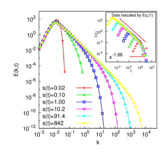
Figure 1: Time evolution of the energy spectrum, $E(k,t)$, of the EDQNM model in the decay case. The main panel shows snapshots of $E(k,t)$ at a succession of times. The inset shows the data collapsed according to Eq. (1) with $a=1.88$ and $s(t)=M_{3}(t)/M_{2}(t)$.

Figure 2: Time evolution of the energy spectrum, $E(k,t)$, of the EDQNM model in the forced case. The main panel shows snapshots of $E(k,t)$ at a succession of times. The inset shows the data collapsed according to Eq. (1) with $a=1.90$ and $s(t)=M_{3}(t)/M_{2}(t)$.

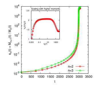
Figure 3: Time evolution of the typical scale, $s_{n}(t)$, as defined by Eq.(3), of the EDQNM model in the forced case for different choices of $n$. The main panel demonstrates that $s_{2}(t)$ and $s_{3}(t)$ show the same qualitative behaviour with a finite time singularity which is regularised by the onset of dissipation. The inset illustrates that the ratio $s_{3}(t)/s_{2}(t)$ is approximately constant as the typical scale (as measured by $s_{2}(t)$) grows over several decades.

We performed simulations of the EDQNM model in the unforced case by integrating numerically Eq. (4), starting from an initial spectrum,

$$E_{k}(0)=Bk^{4}\exp\left[-(k/k_{L})^{2}\right],$$ (14)

with $B$ chosen to normalize the energy to unity and $k_{L}=0.01$. The initial Taylor-scale-Reynolds number is of order $10^{9}$ and the resolution is chosen $24$ gridpoints per decade, logarithmically spaced. A sequence of snapshots of $E_{k}(t)$ before the viscous dissipation became appreciable are shown in Fig. 1. To find the value of the dynamical exponent we should find the value of $a$ which gives the best data collapse under the scaling ansatz, Eq. (1). We defined the typical wavenumber, $s(t)$, to be the ratio, $M_{3}(t)/M_{2}(t)$ of the third to the second moments of the energy spectrum. To find the value of $a$ giving the best data collapse we used the minimization procedure suggested in Bhattacharjee and Seno (2001). Only data with $s(t)>0.2$ were included in the minimization to allow the cascade an entire decade of scales to forget the initial condition (which had $s(0)\approx 0.02$). This procedure gave $1.88\pm 0.04$ where the error estimate is the standard deviation of the distribution of minima obtained by bootstrapping the minimization procedure on randomly selected subsets of the total set of snapshots obtained from the numerical simulation. The data collapse thus obtained, shown in the inset of Fig. 1, is of high quality thereby supporting the scaling ansatz.

Corresponding results for the case of forced turbulence are presented in Fig. 2. The simulation was forced by keeping the energy in the first two wavenumber shells fixed in time. Performing the same analysis on the data as for the unforced case, the optimal data collapse (shown in the inset of Fig. 2) occurs for a value of the dynamical scaling exponent of $1.90\pm 0.05$. This is consistent with the value obtained for the unforced case.

As a final set of checks on the consistency of our numerical simulations with the scaling hypothesis, Eq. (1), Fig. 3 shows the evolution in time (for the forced case) of the typical scale, $s_{n}(t)$ as defined in Eq. (3), for $n=2$ and $n=3$. The fact that $s(t)$ diverges in finite time is clearly evident from the main panel as is the fact that the qualitative behaviour is the same regardless of the choice of $n$. More quantitatively, the inset of Fig. 3 shows that the ratio of the typical scales obtained by taking $n=3$ and $n=2$ is approximately constant over a large range of values of $s_{2}(t)$. The typical scales obtained for different values of $n$ are therefore proportional to each other in the scaling regime, $s(t)\to\infty$ (the subsequent decrease after $s(t)\approx 100$ is due to the onset of dissipation). These results justify our earlier comment that the scaling analysis is insensitive to the choice of ratio of moments used to define the typical scale provided these moments are of sufficiently high order.

Several remarks may be made. Firstly, although there is no a-priori reason why this should be so, the transient exponents measured for the forced and unforced cases are the same within our estimated range of uncertainty. This is quite different from infinite capacity cascades where constraints imposed by conservation laws result in different transient scaling exponents for the forced and unforced cases Connaughton and Krapivsky (2010). Secondly, the measured transient exponents are discernibly different from either of the naive values argued in Eq. (12) or Eq. (11). This confirms our expectation that the transient scaling is different from Kolmogorov. Thirdly, the fact that $a$ is larger than $5/3$ means that the transient spectrum is considerably steeper than the Kolmogorov spectrum. The latter is then set up from right to left in wavenumber space after the onset of dissipation. This transition from the steeper spectrum to $k^{-5/3}$ also evolves quasi-instantaneously in the same sense as the pre-dissipation transient does. It very quickly sets up the usual Kolmogorov spectrum over all scales once the onset of dissipation has occured. This spectrum then decays globally for all subsequent time as detailed, for example, in Lesieur et al. (2005). The EDQNM equation is therefore no different to any of the other finite capacity cascades which have been investigated to date, all of which showed this behaviour. The measured value of the dynamical exponent is remarkably close to the value of $1.86$ measured for the Leith model Connaughton and Nazarenko (2004). This is consistent with recent arguments of Clark et al. Clark et al. (2010) suggesting that the Leith model can be obtained from rational closure models by keeping only a subset of the wavenumber triads.

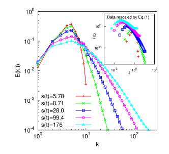
Figure 4: Time evolution of the energy spectrum, $E(k,t)$, in a direct numerical simulation of the decay case. The main panel shows snapshots of $E(k,t)$ at a succession of times. The inset shows the data collapsed according Eq. (1) with $a=1.47$ and $s(t)=M_{3}(t)/M_{2}(t)$.

Given that we expect this kind of transient behaviour to be generic, we close this study with an attempt to measure the corresponding dynamical scaling in a DNS of the full Navier-Stokes equation. A classical Fourier pseudo-spectral method is used to solve the semi-implicit form of the Navier-Stokes equations with tri-periodic boundary conditions, at a resolution of $1024^{3}$ Godeferd and Staquet (2003). Full de-aliasing is performed to remove spurious Fourier coefficients, time marching is done with a third-order Adams-Bashforth explicit scheme, while the viscous term is solved implicitly. The initial velocity conditions consist of a random gaussian field whose energy spectrum is of the form of (14) although with a peak at $k_{L}=4.52$ instead of $0.01$. The results are shown in Fig. 4. Proceeding as described above, we obtained $a=1.47\pm 0.24$. The result is therefore inconclusive as one might expect given the very short scaling range available in DNS data (as compared to numerical solutions of the EDQNM equation).

IV Conclusion

To summarise, we have investigated the self-similar evolution of transient spectra in three dimensional turbulence using numerical solutions of the EDQNM equation and full DNS data. These transients develop before the onset of dissipation and lead to the establishment of the Kolmogorov spectrum. We argued that the self-similarity is of the second kind allowing the transient scaling to be anomalous in the sense that it cannot be determined from dimensional considerations. This is supported by numerical data for the EDQNM equation which gave a transient exponent of $1.88$ compared to the Kolmogorov value of $5/3$. Corresponding measurements for the DNS data were inconclusive owing to the relatively short scaling range available. Nevertheless we would expect, based on our results, that a DNS at sufficiently high Reynolds number would see a steeper transient spectrum. The most relevant message from this work for turbulence research is probably not the value of the transient exponent itself, since few applications care about this early stage regime. Rather it is the fact that such a non-Kolmogorov scaling exists in the first place which serves as a reminder that, while the $k^{-5/3}$ scaling is quite robust when the energy flux through the inertial range is constant, it is not the sole scaling law consistent with the transfer of energy to small scales in turbulence when the constant flux requirement is relaxed.

References

- Galtier et al. (2000) S. Galtier, S. Nazarenko, A. Newell, and A. Pouquet, J. Plasma Phys. 63, 447 (2000).
- Newell et al. (2001) A. Newell, S. Nazarenko, and L. Biven, Physica D 152-153, 520 (2001).
- Connaughton et al. (2003) C. Connaughton, A. Newell, and Y. Pomeau, Physica D 184, 64 (2003).
- Connaughton and Newell (2010) C. Connaughton and A. C. Newell, Phys. Rev. E 81, 036303 (2010).
- Lacaze et al. (2001) R. Lacaze, P. Lallemand, Y. Pomeau, and S. Rica, Physica D 152-153, 779 (2001).
- Connaughton and Pomeau (2004) C. Connaughton and Y. Pomeau, Comptes Rendus Physique 5, 91 (2004).
- Lee (2001) M. Lee, J. Phys. A: Math. Gen. 34, 10219 (2001).
- Galtier et al. (2005) S. Galtier, A. Pouquet, and A. Mangeney, Phys. Plasmas 12, 092310 (2005).
- Barenblatt (1996) G. Barenblatt, Scaling, self-similarity, and intermediate asymptotics (CUP, Cambridge, 1996).
- Leith (1967) C. E. Leith, Phys. Fluids 10, 1409 (1967).
- Connaughton and Nazarenko (2004) C. Connaughton and S. Nazarenko, Phys. Rev. Lett. 92, 044501 (2004).
- Lavoie et al. (2007) P. Lavoie, L. Djenidi, and R. A. Antonia, J. Fluid Mech. 585, 395 (2007).
- Lesieur et al. (2005) M. Lesieur, O. Métais, and P. Comte, Large Eddy Simulations of Turbulence (CUP, Cambridge, 2005).
- Orszag (1970) S. Orszag, J. Fluid Mech. 41, 363 (1970).
- Monin and Yaglom (1975) A. Monin and A. Yaglom, Statistical fluid mechanics (MIT press, Cambridge, 1975).
- Kraichnan (1959) R. Kraichnan, J. Fluid Mech. 5, 497 (1959).
- Clark et al. (2010) T. Clark, R. Rubinstein, and J. Weinstock, J. Turbulence 10, 1 (2010).
- Bos and Bertoglio (2006) W. J. T. Bos and J.-P. Bertoglio, Phys. Fluids 18, 071701 (2006).
- Bos and Bertoglio (2006) W. J. T. Bos and J.-P. Bertoglio, Phys. Fluids 18, 031706 (2006).
- Lesieur (2008) M. Lesieur, Turbulence in Fluids (Springer, Heidelberg, 2008).
- Sagaut and Cambon (2008) P. Sagaut and C. Cambon, Homogeneous turbulence dynamics (CUP, Cambridge, 2008).
- Bhattacharjee and Seno (2001) S. Bhattacharjee and F. Seno, J. Phys. A–Math. Gen. 34, 6375 (2001).
- Connaughton and Krapivsky (2010) C. Connaughton and P. Krapivsky, Phys. Rev. E 81, 035303(R) (2010).
- Godeferd and Staquet (2003) F. S. Godeferd and C. Staquet, J. Fluid Mech. 486, 115 (2003).