Knots in $SU\left(M|N\right)$ Chern-Simons Field Theory

Abstract

Knots in the Chern-Simons field theory with Lie super gauge group $SU\left(M|N\right)$ are studied, and the $S_{L}\left(\alpha,\beta,z\right)$ polynomial invariant with skein relations are obtained under the fundamental representation of $\mathfrak{su}\left(M|N\right)$.

PACS Numbers: 11.15.-q, 02.10.Kn

Keywords: Chern-Simons Field Theory; Lie supergroup $SU\left(M|N\right)$; Link Invariants.

1 Introduction

Chern-Simons (CS) theories are Schwarz-type topological field theories — a CS action is both gauge invariant and generally covariant, and a quantum CS theory has general variance in the BRST formalism under the Landau gauge although a metric enters the gauge-fixing term [1]. CS theories were first introduced into physics in the study of quantum anomaly of gauge symmetries by Jackiw et al. [2]. Witten pointed out [3] that CS theories provide a field theoretical origin for polynomial invariants of links in knot theory. Different Lie gauge groups of the CS theories and different algebraic representations of the gauge groups lead to different link invariants [3, 4, 5]. Perturbative expansions of correlation functions of Wilson loops in CS theories present Vassiliev invariants [6, 7, 8]. Recent developments include the applications of CS theories in topological string theory [9] and the $\left(2+1\right)$-dimensional quantum gravity [10].

Super symmetries have found realizations in various physical systems [11]. Representation theories for Lie superalgebras have been developed by many authors [12, 13]. Link invariants have been obtained from quantum super group invariants by Gould, Bracken, Zhang, Links, Kauffman, et al. from the algebraic point of view [14], including the HOMFLY polynomial from the $U_{q}\left(\mathfrak{su}\left(M|N\right)\right)$ invariants $\left(M\neq N\right)$, the Kauffman polynomial from the $U_{q}\left(\mathfrak{osp}\left(M|2N\right)\right)$ invariants, and the Alexander-Conway polynomial from the $U_{q}\left(\mathfrak{gl}\left(N|N\right)\right)$ invariants.

In this paper we will use the field theoretical point of view to study knots in the CS field theory with super gauge group $SU\left(M|N\right),\ M\neq N$ [15, 16]. Under the fundamental representation of the superalgebra $\mathfrak{su}\left(M|N\right)$, a correlation function of Wilson loop operators will be studied and the $S_{L}\left(\alpha,\beta,z\right)$ link polynomial be obtained [4]. One will discuss the relationships between the $S_{L}\left(\alpha,\beta,z\right)$ polynomial and the HOMFLY and Jones polynomials, and show that the CS theory with super group $SU\left(N+2|N\right)$ has the Jones polynomial invariant. This is different from the situation of the CS theory with normal Lie group $SU\left(N\right)$ — under the fundamental representation, only the $SU\left(2\right)$ CS theory has the Jones polynomial.

This paper is arranged as follows. In Section 2, the notation of Lie superalgebra $\mathfrak{su}\left(M|N\right)$ under the fundamental representation is given. In Section 3, path variation within correlation functions of Wilson loops in the CS theory is rigorously studied. In Section 4, the variation of correlation functions obtained in Section 3 is formally discussed with respect to different link configurations, without integrating out the path integrals. From the formal analysis the $S_{L}\left(\alpha,\beta,z\right)$ polynomial with skein relations is obtained, and its relationships to other knot polynomials are discussed. The paper is summarized in Section 5.

2 Notation and Preliminary

Let us fix the notation of the superalgebra $\mathfrak{su}\left(M|N\right)$ first. Consider the elements $\left\{\left.\hat{e}_{ab}\right|a,b=1,\cdots,M+N,\ M\neq N\right\}$ satisfying the following super commutation relations [17, 18, 19, 20]:

$$\left[\hat{e}_{ab},\hat{e}_{cd}\right]=\hat{e}_{ad}\delta_{bc}-\left(-1\right)^{\left(\left[a\right]+\left[b\right]\right)\left(\left[c\right]+\left[d\right]\right)}\hat{e}_{cb}\delta_{da}.$$ (1)

Here the $\mathbb{Z}_{2}$-grading is given by $\left[\hat{e}_{ab}\right]=\left[a\right]+\left[b\right]$ with $\left[1\right]=\cdots=\left[M\right]=0$ and $\left[M+1\right]=\cdots=\left[M+N\right]=1$. In the fundamental representation $\hat{e}_{ab}$ is realized by

$$\hat{e}_{ab}=e_{ab}-\frac{\delta_{ab}\left(-1\right)^{\left[a\right]}}{M-N}I,$$ (2)

where $e_{ab}$ is the $\left(M+N\right)\times\left(M+N\right)$ matrix unit with entry $1$ at the position $\left(a,b\right)$ and $0$ elsewhere. $\hat{e}_{ab}$ satisfies the traceless requirement $Str\left(\hat{e}_{ab}\right)=0,$ where $Str\left(X\right)$ is the supertrace of the representation matrix of $X\in\mathfrak{g}$, $Str\left(X\right)=\sum_{i}\left(-1\right)^{\left[i\right]}X_{ii}$, $i$ denoting the entry indices. The $\hat{e}_{ab}$’s have the identity $\sum_{a=1}^{M+N}\hat{e}_{aa}=0$. The $\left(M+N\right)^{2}-1$ generators of the supergroup $SU\left(M|N\right)$, denoted by $\left\{\hat{E}_{ab},\hat{F}_{ab},\hat{H}_{cc}\right\}$, can be constructed in terms of $\hat{e}_{ab}$:

$$\begin{array}[]{ll}\hat{E}_{ab}=\frac{i}{2}\left(\hat{e}_{ab}-\hat{e}_{ba}\right),\ \hat{F}_{ab}=\frac{1}{2}\left(\hat{e}_{ab}+\hat{e}_{ba}\right),&\ \ \ a,b=1,\cdots,M+N,\ a\neq b;\\ \hat{H}_{cc}=\sum_{l=1}^{c}l\left(\hat{e}_{ll}-\hat{e}_{l+1,l+1}\right),&\ \ \ c=1,\cdots,M+N-1,\end{array}$$ (3)

where no summation for repeating $c,l$. The $\hat{E}_{ab},\hat{F}_{ab}$ and $\hat{H}_{cc}$ satisfy the properties of tracelessness and unitarity: $Str\left(\hat{E}_{ab}\right)=Str\left(\hat{F}_{ab}\right)=Str\left(\hat{H}_{cc}\right)=0$; $\left(\hat{E}_{ab}\right)^{{\dagger}}=\hat{E}_{ab}$, $\left(\hat{F}_{ab}\right)^{{\dagger}}=\hat{F}_{ab}$ and $\left(\hat{H}_{cc}\right)^{{\dagger}}=\hat{H}_{cc}$. The $\hat{E}_{ab}$ and $\hat{F}_{ab}$ play the role of the raising/lowering generators, and $\hat{H}_{cc}$ the elements of the Cartan subalgebra of $\mathfrak{su}\left(M|N\right)$. Hereinafter for convenience one uses the basis $\left\{\hat{e}_{ab},\ a\neq b;\ \ \hat{e}_{cc},\ c=1,\cdots,M+N-1\right\}$.

We begin the study of the knots in a CS field theory by considering the correlation function of Wilson loops under the fundamental representation of $\mathfrak{su}\left(M|N\right)$ [3, 4, 5]

$$\left\langle W\left(L\right)\right\rangle=\left\langle StrPe^{i\oint_{L}A_{\mu}\left(x\right)dx^{\mu}}\right\rangle=Z^{-1}StrP\int\mathcal{D}Ae^{iS}e^{i\oint_{L}A_{\mu}\left(x\right)dx^{\mu}},$$ (4)

where $Z=\int\mathcal{D}Ae^{iS}$ the normalization factor. $L$ denotes the integration loop and $P$ the proper product. $S$ is the non-Abelian CS action,

$$S=\frac{k}{4\pi}\int_{\mathbb{R}^{3}}d^{3}x\epsilon^{\mu\nu\rho}Str\left(A_{\mu}\partial_{\nu}A_{\rho}+\frac{2}{3}A_{\mu}A_{\nu}A_{\rho}\right),$$ (5)

$k$ being an integer valued constant. $A_{\mu}$ is the $SU(M|N)$ gauge potential, $A_{\mu}=A_{\mu}^{ab}\hat{e}_{ab}$. The gauge field tensor $F_{\mu\nu}$ is induced by $A_{\mu}:$

$$F_{\mu\nu}=F_{\mu\nu}^{ab}\hat{e}_{ab},\ \ \ \ \ \ \ \ \ F_{\mu\nu}^{ab}=\partial_{\mu}A_{\nu}^{ab}-\partial_{\nu}A_{\mu}^{ab}-\left(-1\right)^{\left(\left[a\right]+\left[c\right]\right)\left(\left[c\right]+\left[b\right]\right)}\left(A_{\mu}^{ac}A_{\nu}^{cb}-A_{\nu}^{ac}A_{\mu}^{cb}\right).$$ (6)

The grading $\left[A_{\mu}\right]=\left[F_{\mu\nu}\right]=\left[S\right]=\mathrm{even}$.

The gauge invariance of the phase of the action, $e^{iS}$, needs more discussion. The gauge transformations of $A_{\mu}$ and $F_{\mu\nu}$ are $A_{\mu}\longrightarrow\Omega A_{\mu}\Omega^{-1}+\partial_{\mu}\Omega\Omega^{-1}$ and $F_{\mu\nu}\longrightarrow\Omega F_{\mu\nu}\Omega^{-1},$ with $\Omega$ denoting a group $G$ transformation. It is known that if $G$ is a normal Lie group the action $S$ transforms as

$$S\longrightarrow S+\frac{k}{4\pi}\int_{\mathbb{R}^{3}}d^{3}x\partial_{\mu}j^{\mu}+2\pi k\frac{1}{24\pi^{2}}\int_{\mathbb{R}^{3}}d^{3}x\epsilon^{\mu\nu\rho}Str\left[a_{\mu}a_{\nu}a_{\rho}\right],$$ (7)

where $a_{\mu}=\Omega^{-1}\partial_{\mu}\Omega$ and $j^{\mu}=\epsilon^{\mu\nu\rho}Str\left(A_{\nu}a_{\rho}\right)$. The second term in (7) is a total divergence which has no contribution to the action as $j^{\mu}$ vanishes at infinity. The third term, marked as $S_{\mathrm{WZW}}$, is a Wess-Zumino-Witten (WZW) term. Jackiw, Cronström, Mickelsson, et al. [2, 21] examined this term for an arbitrary non-Abelian Lie group $G$. They pointed out that when $\Omega$ satisfies the regular condition — $\Omega$ tends to a definite limit at infinity, $\lim_{\mathbf{x}\rightarrow\infty}\Omega\left(\mathbf{x}\right)=I$ — the WZW term is a total differential

$$S_{\mathrm{WZW}}=2\pi k\frac{1}{24\pi^{2}}\int_{\mathbb{R}^{3}}dx^{\mu}\partial_{\mu}\left[\Theta_{\nu\rho}dx^{\nu}\wedge dx^{\rho}\right]=2\pi k\frac{1}{\pi^{2}}\int_{\mathbb{R}^{3}}d\Theta,$$ (8)

where $\Theta$ is a $2$-form constructed by $\Omega$, and $d\Theta$ serves as a volume element [21]. Since the regular condition implies the compactification $\mathbb{R}^{3}\longrightarrow S^{3}$, Eq.(8) becomes $S_{\mathrm{WZW}}=2\pi k\frac{1}{\pi^{2}}\int_{S^{3}}d\Theta$, which gives the degree of the homotopy mapping $\Omega:S^{3}\rightarrow G$ when $G$ is compact. Hence for a compact group $G$ one has $S_{\mathrm{WZW}}=2\pi kw\left(\Omega\right)$, and the action transforms as $S\rightarrow S+2\pi kw\left(\Omega\right)$, where $w\left(\Omega\right)$ is the so-called winding number, $w\left(\Omega\right)\in\pi_{3}\left[SU\left(M|N\right)\right]=\mathbb{Z}$. In this paper, the gauge group is the super group $SU\left(M|N\right)$; a point needs clarification is whether the WZW term is able to be written as a total differential. This problem is being studied by us at present and will be discussed in our further papers.

Under the fundamental representation (2) the $\hat{e}_{ab}$ has the following supertraces

$$Str\left(\hat{e}_{ab}\hat{e}_{cd}\right) = \left(-1\right)^{\left[a\right]}\delta_{ad}\delta_{bc}-\frac{\left(-1\right)^{\left[a\right]+\left[c\right]}\delta_{ab}\delta_{cd}}{M-N},$$ (9)

$$Str\left(\hat{e}_{ab}\hat{e}_{cd}\hat{e}_{ef}\right) = \left(-1\right)^{\left[a\right]}\delta_{af}\delta_{bc}\delta_{de}-\left(-1\right)^{\left[a\right]+\left[c\right]}\frac{\delta_{ab}\delta_{cf}\delta_{de}}{M-N}-\left(-1\right)^{\left[c\right]+\left[f\right]}\frac{\delta_{cd}\delta_{af}\delta_{be}}{M-N}$$ (10)

$$-\left(-1\right)^{\left[f\right]+\left[a\right]}\frac{\delta_{ef}\delta_{ad}\delta_{bc}}{M-N}+2\left(-1\right)^{\left[a\right]+\left[c\right]+\left[e\right]}\frac{\delta_{ab}\delta_{cd}\delta_{ef}}{\left(M-N\right)^{2}}.$$

In terms of (9) and (10) the component form of the $SU\left(M|N\right)$ CS action reads

$$S = \frac{k}{4\pi}\int d^{3}x\epsilon^{\mu\nu\rho}\left(-1\right)^{\left[b\right]}$$ (11)

$$\left[A_{\mu}^{ab}\partial_{\nu}A_{\rho}^{ba}+\frac{2}{3}\left(-1\right)^{\left[c\right]+\left[a\right]\left[b\right]+\left[b\right]\left[c\right]+\left[c\right]\left[a\right]}A_{\mu}^{ab}A_{\nu}^{bc}A_{\rho}^{ca}-\left(-1\right)^{\left[a\right]}\frac{A_{\mu}^{aa}\partial_{\nu}A_{\rho}^{bb}}{M-N}\right.$$

$$\left.-\frac{2}{3}\left(-1\right)^{\left[a\right]}\frac{A_{\mu}^{aa}A_{\nu}^{cb}A_{\rho}^{bc}}{M-N}+\frac{4}{3}\left(-1\right)^{\left[a\right]+\left[c\right]}\frac{A_{\mu}^{aa}A_{\nu}^{bb}A_{\rho}^{cc}}{\left(M-N\right)^{2}}\right].$$

It can be proved that $S$ has an important property [5, 4, 1]

$$\frac{2\pi}{k}\epsilon^{\mu\nu\rho}\left(-1\right)^{\left[b\right]}\frac{\partial S}{\partial A_{\rho}^{ab}\left(x\right)}\hat{e}_{ba}=F_{\mu\nu}^{ba}\left(x\right)\hat{e}_{ba}.$$ (12)

This gives the equation of motion of a pure gauge: $\frac{2\pi}{k}\frac{\delta S}{\delta A}=F=0$, which is the same as the commonly known equation of motion in the CS theories with normal Lie gauge groups. Eq.(12) will be crucial in following sections for derivation of the skein relations of knots in the CS theory with $SU\left(M|N\right)$ gauge group.

3 Variation of Correlation Function

In this section correlation functions of Wilson loops will be studied, with emphasis placed on variation of integration paths and the induced changes of the correlation functions.

Consider two knots which are almost the same except at one double-point $x_{0}$, as illustrated by Figure 1.

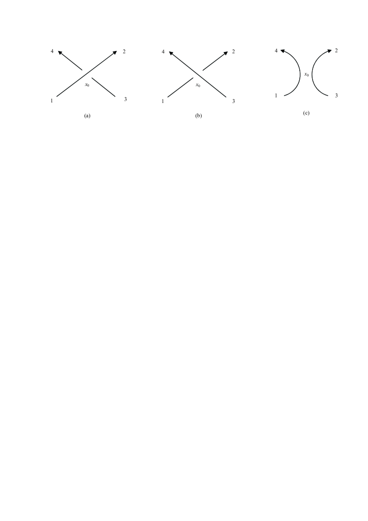
Figure 1: Overcrossing, Undercrossing and Non-Crossing: (a) $L_{+}$; (b) $L_{-}$; (c) $L_{0}$.

Here $1,2,3,4$ are the abbreviations for the points $x_{1},x_{2},x_{3},x_{4}$. Denote the knot in Figure 1(a) as $L_{+}$ and that in Figure 1(b) as $L_{-}$. Figure 1(c) shows the non-crossing situation. Let $U\left(1,2\right)$ [resp. $U\left(3,4\right)$] be the propagation process along the segment $\left(1\rightarrow 2\right)$ [resp. $\left(3\rightarrow 4\right)$]. For convenience denote the $U\left(1,2\right)$ in Figure 1(a) as $U_{+}\left(1,2\right)$, and that in Figure 1(b) as $U_{-}\left(1,2\right)$. In both Figures 1(a) and 1(b), the process $\left(1\rightarrow 2\right)$ is prior to $\left(3\rightarrow 4\right)$ in the sense of proper order. In following we will discuss the difference between the overcrossing $L_{+}$ and undercrossing $L_{-}$, by fixing the segment $\left(3\rightarrow 4\right)$ and moving the segment $\left(1\rightarrow 2\right)$ from back to front.

Let $\left\langle W\left(L_{+}\right)\right\rangle\$and $\left\langle W\left(L_{-}\right)\right\rangle$ be the respective correlation functions of $L_{+}$ and $L_{-}$. Each of them can be written as a series of propagation processes in proper order:

$$\left\langle W\left(L_{\pm}\right)\right\rangle=\left\langle Str\left[\cdots U_{\pm}\left(1,2\right)\cdots U\left(3,4\right)\cdots\right]\right\rangle,$$ (13)

where the propagators are realized by

$$U_{\pm}\left(1,2\right)=\left.e^{i\int_{1}^{2}A_{\mu}\left(x\right)dx^{\mu}}\right|_{L_{\pm}},\ \ \ \ \ \ \ \ \ U\left(3,4\right)=e^{i\int_{3}^{4}A_{\mu}\left(x\right)dx^{\mu}},$$ (14)

the grading of $U_{\pm}\left(1,2\right)$ and $U\left(3,4\right)$ being even. The difference between the correlation functions of $L_{+}$ and $L_{-}$ is

$$\left\langle W\left(L_{+}\right)\right\rangle-\left\langle W\left(L_{-}\right)\right\rangle=\left\langle Str\left(\cdots\left[U_{+}\left(1,2\right)-U_{-}\left(1,2\right)\right]\cdots U\left(3,4\right)\cdots\right)\right\rangle.$$ (15)

The path variation $L_{-}\rightarrow L_{+},$ given by $\left[U_{+}\left(1,2\right)-U_{-}\left(1,2\right)\right]$ in (15), is stereoscopically illustrated in Figure 2, where the segment $\left(1\rightarrow 2\right)$ in $L_{-}$ corresponds to the path $\overline{\mathrm{1ACDB2}}$, and that in $L_{+}$ to $\overline{\mathrm{1AEFB2}}$.

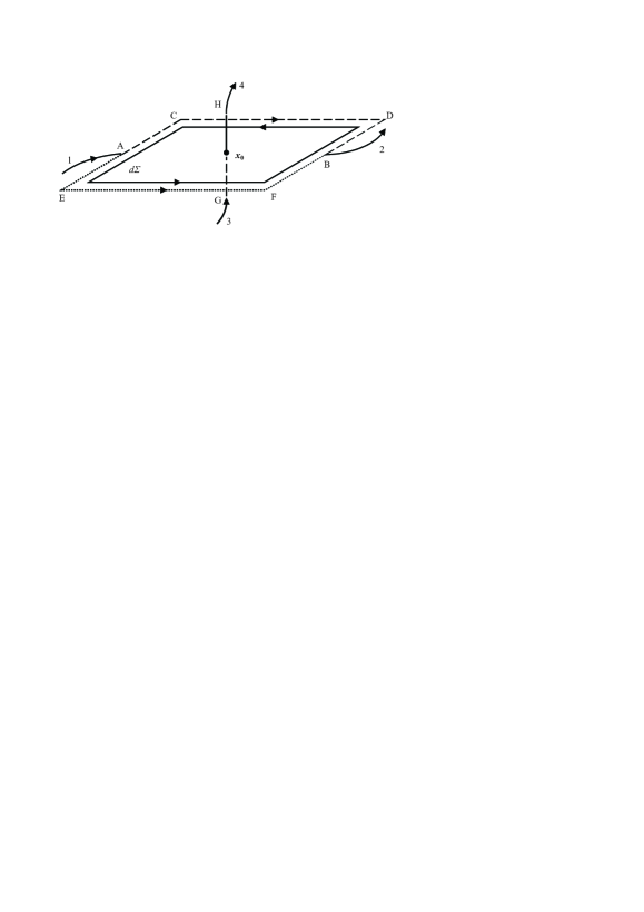
Figure 2: $3$-Dimensional Geometric Illustration of Path Variation

Then

$$U_{+}\left(1,2\right)-U_{-}\left(1,2\right)=U\left(1,A\right)\left(i\int_{\overline{\mathrm{AEFB}}}A_{\mu}\left(x\right)dx^{\mu}-i\int_{\overline{\mathrm{ACDB}}}A_{\mu}\left(x\right)dx^{\mu}\right)U\left(B,2\right),$$ (16)

where the exponential expansion $e^{i\int A_{\mu}\left(x\right)dx^{\mu}}=1+i\int A_{\mu}\left(x\right)dx^{\mu}$ applies. In the light of the Stokes’ law one has

$$U_{+}\left(1,2\right)-U_{-}\left(1,2\right)=U\left(1,A\right)\left(i\int_{\partial\framebox{{\tiny AEFBDC}}}A_{\mu}\left(x\right)dx^{\mu}\right)U\left(B,2\right)$$ (17)

$$= U\left(1,A\right)\left(i\int_{\framebox{{\tiny AEFBDC}}}\frac{1}{2}F_{\mu\nu}\left(x\right)dx^{\mu}\wedge dx^{\nu}\right)U\left(B,2\right),$$

where $\partial\framebox{{\tiny AEFBDC}}$ is the boundary of the tiny area AEFBDC at $x_{0}$. In (17) the curvature $F_{\mu\nu}\left(x\right)$ is the $SU\left(M|N\right)$ gauge field tensor which has the expansion $F_{\mu\nu}\left(x\right)=F_{\mu\nu}^{ab}\left(x\right)\hat{e}_{ab}$.

Thus the difference between the path integrals $\left\langle W\left(L_{-}\right)\right\rangle$ and $\left\langle W\left(L_{+}\right)\right\rangle$ is

$$\left\langle W\left(L_{+}\right)\right\rangle-\left\langle W\left(L_{-}\right)\right\rangle$$ (18)

$$= Z^{-1}\int_{\framebox{{\tiny AEFBDC}}}\frac{1}{2}dx^{\mu}\wedge dx^{\nu}\int\mathcal{D}Ae^{iS}$$

$$Str\left[\cdots U\left(1,A\right)iF_{\mu\nu}^{ab}\left(x\right)\hat{e}_{ab}U\left(B,2\right)\cdots U\left(3,4\right)\cdots\right].$$

Using the property of the Chern-Simons action (12), one has

$$\left\langle W\left(L_{+}\right)\right\rangle-\left\langle W\left(L_{-}\right)\right\rangle$$ (19)

$$= \frac{2\pi}{k}Z^{-1}\int_{\framebox{{\tiny AEFBDC}}}d\Sigma^{\rho}\int\mathcal{D}A$$

$$Str\left[\cdots U\left(1,A\right)\left(-1\right)^{\left[a\right]}\hat{e}_{ba}\frac{\partial e^{iS}}{\partial A_{\rho}^{ab}\left(x\right)}U\left(B,2\right)\cdots U\left(3,4\right)\cdots\right]$$

$$= -\frac{2\pi}{k}Z^{-1}\int_{\framebox{{\tiny AEFBDC}}}d\Sigma^{\rho}\int\mathcal{D}Ae^{iS}$$

$$Str\left[\cdots U\left(1,A\right)\left(-1\right)^{\left[a\right]}\hat{e}_{ba}U\left(B,2\right)\frac{\partial}{\partial A_{\rho}^{ab}\left(x\right)}\left[\cdots U\left(3,4\right)\cdots\right]\right],$$

where $d\Sigma^{\rho}=\frac{1}{2}\epsilon^{\rho\mu\nu}dx^{\mu}\wedge dx^{\nu}$ is the surface element of AEFBDC, and the technique of integration by parts has been used. In (19) the propagators $\left[\cdots U\left(1,A\right)\hat{e}_{ba}U\left(B,2\right)\right]$ are taken out of the derivative $\frac{\partial}{\partial A_{\rho}^{ab}\left(x\right)}$ because they are not impacted by the move of Figure 2. In the remaining propagation processes $\left[\cdots U\left(3,4\right)\cdots\right]$, only $\left(3\rightarrow 4\right)$ passes the point $x_{0}$, hence only $U\left(3,4\right)$ is impacted by the move. Therefore,

$$\left\langle W\left(L_{+}\right)\right\rangle-\left\langle W\left(L_{-}\right)\right\rangle$$ (20)

$$= -\frac{2\pi}{k}Z^{-1}\int_{\framebox{{\tiny AEFBDC}}}d\Sigma^{\rho}\int\mathcal{D}Ae^{iS}\cdot$$

$$Str\left[\cdots U\left(1,A\right)\left(-1\right)^{\left[a\right]}\hat{e}_{ba}U\left(B,2\right)\cdots\left(\frac{\partial}{\partial A_{\rho}^{ab}\left(x\right)}U\left(3,4\right)\right)\cdots\right].$$

Let us examine the $\left(\frac{\partial}{\partial A_{\rho}^{ab}\left(x\right)}U\left(3,4\right)\right)$ in (20). It is shown in Figure 2 that

$$U\left(3,4\right)=e^{i\int_{3}^{4}A_{\lambda}\left(y\right)dy^{\lambda}}=U\left(3,G\right)e^{\int_{G}^{H}iA_{\lambda}^{kl}\left(y\right)\hat{e}_{kl}dy^{\lambda}}U\left(H,4\right),$$ (21)

where $\overline{\mathrm{GH}}$ is a short segment passing $x_{0}$. Thus

$$\frac{\partial}{\partial A_{\rho}^{ab}\left(x\right)}U\left(3,4\right)=U\left(3,G\right)\left[\int_{G}^{H}i\delta^{3}\left(x-x_{0}\right)dx^{\rho}\hat{e}_{ab}e^{\int_{G}^{H}iA_{\lambda}^{kl}\left(y\right)\hat{e}_{kl}dy^{\lambda}}\right]U\left(H,4\right),$$ (22)

and (20) becomes

$$\left\langle W\left(L_{+}\right)\right\rangle-\left\langle W\left(L_{-}\right)\right\rangle$$ (23)

$$= -i\frac{2\pi}{k}Z^{-1}\int_{\framebox{{\tiny AEFBDC}}}\int_{G}^{H}\delta^{3}\left(x-x_{0}\right)d\Sigma^{\rho}\otimes dx^{\rho}\int\mathcal{D}Ae^{iS}\cdot$$

$$Str\left[\cdots U\left(1,A\right)\left(-1\right)^{\left[a\right]}\hat{e}_{ba}U\left(B,2\right)\cdots U\left(3,x_{0}\right)\hat{e}_{ab}U\left(x_{0},4\right)\cdots\right],$$

where the $dx^{\rho}$ is along the direction of the segment $\overline{\mathrm{GH}}$. In (23) a volume integral is recognized:

$$\left[\text{vol}\right]_{x_{0}}=\int_{\framebox{{\tiny AEFBDC}}}\int_{G}^{H}\delta^{3}\left(x-x_{0}\right)d\Sigma^{\rho}\otimes dx^{\rho},$$ (24)

which has the evaluation

$$\left[\text{vol}\right]_{x_{0}}\left\{\begin{array}[]{ll}=0,&\text{trivial;}\\ =\pm 1,&\text{non-trivial.}\end{array}\right.$$ (25)

In detail,

• $\left[\text{vol}\right]_{x_{0}}=0$ describes the trivial case that in Figure 2 the $dx^{\rho}$ is parallel to the plane of AEFBDC; namely, the move from $\overline{\mathrm{ACDB}}$ to $\overline{\mathrm{AEFB}}$ is done by sliding along $\overline{\mathrm{3GH4}}$. Therefore $d\Sigma^{\rho}\otimes dx^{\rho}=0$.

• $\left[\text{vol}\right]_{x_{0}}=1$ describes the non-trivial move $L_{-}\rightarrow$ $L_{+}$, where $dx^{\rho}$ is perpendicular to AEFBDC and $d\Sigma^{\rho}\otimes dx^{\rho}=1$; otherwise, $\left[\text{vol}\right]_{x_{0}}=-1$ for $L_{+}\rightarrow$ $L_{-}$, where $dx^{\rho}$ is perpendicular to AEFBDC but $d\Sigma^{\rho}\otimes dx^{\rho}=-1$. The case we come across in Figure 2 is the former, so $\left[\text{vol}\right]_{x_{0}}=1$.

Therefore, (23) becomes

$$\left\langle W\left(L_{+}\right)\right\rangle-\left\langle W\left(L_{-}\right)\right\rangle$$ (26)

$$= -i\frac{2\pi}{k}Z^{-1}\int\mathcal{D}Ae^{iS}$$

$$Str\left[\cdots U\left(1,A\right)\left(-1\right)^{\left[b\right]}\hat{e}_{ab}U\left(B,2\right)\cdots U\left(3,x_{0}\right)\hat{e}_{ba}U\left(x_{0},4\right)\cdots\right].$$

4 Skein Relations

In this section the $S_{L}\left(\alpha,\beta,z\right)$ polynomial invariant for knots in the $SU\left(M|N\right)$ CS field theory will be derived from (26), and its relationship to the HOMFLY and Jones polynomials will be discussed.

Under the fundamental representation the entries of the matrices $\hat{e}_{ab}$ satisfy the Fierz identity [22]

$$\left(-1\right)^{\left[b\right]}\left(\hat{e}_{ab}\right)_{ij}\left(\hat{e}_{ba}\right)_{kl}=\left(-1\right)^{\left[j\right]}\delta_{il}\delta_{jk}-\frac{1}{M-N}\delta_{ij}\delta_{kl}.$$ (27)

Hence (26) leads to

$$\left\langle W\left(L_{+}\right)\right\rangle-\left\langle W\left(L_{-}\right)\right\rangle$$ (28)

$$= -i\frac{2\pi}{k}Z^{-1}\int\mathcal{D}Ae^{iS}\cdot$$

$$Str\left[\cdots U\left(1,A\right)U\left(x_{0},4\right)\cdots\right]Str\left[U\left(B,2\right)\cdots U\left(3,x_{0}\right)\right]$$

$$+i\frac{2\pi}{k}\frac{1}{M-N}Z^{-1}\int\mathcal{D}Ae^{iS}\cdot$$

$$Str\left[\cdots U\left(1,A\right)U\left(B,2\right)\cdots U\left(3,x_{0}\right)U\left(x_{0},4\right)\cdots\right].$$

When the points $A$ and $B$ approaching $x_{0}$, the first term of (28) corresponds to the non-crossing case $L_{0}$ in Figure 1(c). For the second term, however, one has two ways to connect $A$ and $B$ — the undercrossing and the overcrossing — in order to form a propagation process $\left(1\rightarrow 2\right)$. Treating these two crossing ways equally, one has

$$\left(1-i\frac{\pi}{k}\frac{1}{\left(M-N\right)}\right)\left\langle W\left(L_{+}\right)\right\rangle-\left(1+i\frac{\pi}{k}\frac{1}{\left(M-N\right)}\right)\left\langle W\left(L_{-}\right)\right\rangle=-i\frac{2\pi}{k}\left\langle W\left(L_{0}\right)\right\rangle.$$ (29)

Then, considering the weak coupling limit of large $k$ [3], we define

$$\beta=1-i\frac{\pi}{k}\frac{1}{\left(M-N\right)}+O\left(\frac{1}{k^{2}}\right),\ \ \ \ \ z=-i\frac{2\pi}{k}+O\left(\frac{1}{k^{2}}\right),$$ (30)

and obtain an important skein relation

$$\beta\left\langle W\left(L_{+}\right)\right\rangle-\beta^{-1}\left\langle W\left(L_{-}\right)\right\rangle=z\left\langle W\left(L_{0}\right)\right\rangle.$$ (31)

For the purpose of examining knot writhing, let us consider the special case that the point $x_{2}$ is identical to $x_{3}$ in Figure 1. Then in (26) one has

$$\lim_{B\rightarrow x_{0};x_{2}=x_{3}}U\left(B,2\right)\cdots U\left(3,x_{0}\right)=I,$$ (32)

and

$$\left\langle W\left(\hat{L}_{+}\right)\right\rangle-\left\langle W\left(\hat{L}_{-}\right)\right\rangle$$ (33)

$$= -i\frac{2\pi}{k}Z^{-1}\int\mathcal{D}Ae^{iS}Str\left[\cdots U\left(1,A\right)\left(-1\right)^{\left[b\right]}\hat{e}_{ab}\hat{e}_{ba}U\left(x_{0},4\right)\cdots\right],$$

where $\hat{L}_{+}$ and $\hat{L}_{-}$ are two writhing situations shown in Figure 3(a) and 3(b). Figure 3(c) shows the non-writhing situation $\hat{L}_{0}$.

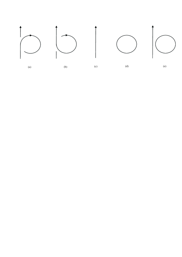
Figure 3: Typical Configurations: (a) writhing $\hat{L}_{+}$; (b) writhing $\hat{L}_{-}$; (c) non-writhing $\hat{L}_{0}$; (d) trivial circle $\hat{L}_{c}$; (e) non-intersecting union $\hat{L}_{i}$.

In the above the factor $\left(-1\right)^{\left[b\right]}\hat{e}_{ab}\hat{e}_{ba}$ is the Casimir operator

$$\left(-1\right)^{\left[b\right]}\hat{e}_{ab}\hat{e}_{ba}=2C_{2}I,\ \ \ \ \ \ \ \ C_{2}=\frac{\left(M-N\right)^{2}-1}{2\left(M-N\right)},\ \ M\neq N.$$ (34)

When $A$ approaches $x_{0}$ one has

$$\left\langle W\left(\hat{L}_{+}\right)\right\rangle-\left\langle W\left(\hat{L}_{-}\right)\right\rangle=-i\frac{4\pi}{k}C_{2}\left\langle W\left(\hat{L}_{0}\right)\right\rangle,$$ (35)

where $\left\langle W\left(\hat{L}_{0}\right)\right\rangle=Z^{-1}\int\mathcal{D}Ae^{iS}Str\left[\cdots U\left(1,x_{0}\right)U\left(x_{0},4\right)\cdots\right]$. The move $\hat{L}_{-}\rightarrow$ $\hat{L}_{+}$ is a change of the writhe of the path segment. In this regard an intermediate stage $\hat{L}_{0}$ can be inserted and the move becomes $\hat{L}_{-}\rightarrow$ $\hat{L}_{0}\rightarrow$ $\hat{L}_{+}$. Then the correlation function becomes $\left\langle W\left(\hat{L}_{+}\right)\right\rangle-\left\langle W\left(\hat{L}_{-}\right)\right\rangle=\left[\left\langle W\left(\hat{L}_{+}\right)\right\rangle-\left\langle W\left(\hat{L}_{0}\right)\right\rangle\right]+\left[\left\langle W\left(\hat{L}_{0}\right)\right\rangle-\left\langle W\left(\hat{L}_{-}\right)\right\rangle\right].$ The two subprocesses $\hat{L}_{-}\rightarrow\hat{L}_{0}$ and $\hat{L}_{0}\rightarrow$ $\hat{L}_{+}$ should be equivalent, hence
$\left\langle W\left(\hat{L}_{+}\right)\right\rangle-\left\langle W\left(\hat{L}_{0}\right)\right\rangle=\left\langle W\left(\hat{L}_{0}\right)\right\rangle-\left\langle W\left(\hat{L}_{-}\right)\right\rangle=-i\frac{2\pi}{k}C_{2}\left\langle W\left(\hat{L}_{0}\right)\right\rangle$, and we arrive at another skein relation

$$\left\langle W\left(\hat{L}_{+}\right)\right\rangle=\alpha\left\langle W\left(\hat{L}_{0}\right)\right\rangle,\ \ \left\langle W\left(\hat{L}_{-}\right)\right\rangle=\alpha^{-1}\left\langle W\left(\hat{L}_{0}\right)\right\rangle,\ \ \alpha=1-i\frac{2\pi}{k}C_{2}+O\left(\frac{1}{k^{2}}\right).$$ (36)

Besides (31) and (36), one needs the correlation function for the trivial circle $\hat{L}_{c}$ shown in Figure 3(d):

$$\left\langle W\left(\hat{L}_{c}\right)\right\rangle=Z^{-1}\int\mathcal{D}Ae^{iS}Str\left[\hat{L}_{c}\right]=Z^{-1}\int\mathcal{D}Ae^{iS}Str\left[I\right]=\left(M-N\right).$$ (37)

Thus, in summary, we have acquired the following skein relations for knots in the $SU\left(M|N\right)$ CS field theory:

$$\left\langle W\left(\hat{L}_{c}\right)\right\rangle=M-N\ \ \ \ \ \ \ \ \ \ \ \ \ \ \left(M\neq N\right),$$ (38)

$$\left\langle W\left(\hat{L}_{+}\right)\right\rangle=\alpha\left\langle W\left(\hat{L}_{0}\right)\right\rangle,\ \ \ \ \left\langle W\left(\hat{L}_{-}\right)\right\rangle=\alpha^{-1}\left\langle W\left(\hat{L}_{0}\right)\right\rangle,$$ (39)

$$\beta\left\langle W\left(L_{+}\right)\right\rangle-\beta^{-1}\left\langle W\left(L_{-}\right)\right\rangle=z\left\langle W\left(L_{0}\right)\right\rangle,$$ (40)

with

$$\alpha=1-i\frac{2\pi}{k}C_{2}+O\left(\frac{1}{k^{2}}\right),\ \ \ \beta=1-i\frac{\pi}{k}\frac{1}{\left(M-N\right)}+O\left(\frac{1}{k^{2}}\right),\ \ \ z=-i\frac{2\pi}{k}+O\left(\frac{1}{k^{2}}\right).$$ (41)

These relations present a polynomial invariant $\left\langle W\left(L\right)\right\rangle$ for the knots, known as the $S_{L}\left(\alpha,\beta,z\right)$ polynomial proposed by Guadagnini et al. [4, 1].

It is checked that Eq.(39) is consistent with (40). Considering the special case $x_{2}=x_{3}$ for (31) there is

$$\beta\left\langle W\left(\hat{L}_{+}\right)\right\rangle-\beta^{-1}\left\langle W\left(\hat{L}_{-}\right)\right\rangle=z\left\langle W\left(\hat{L}_{i}\right)\right\rangle,$$ (42)

where $\hat{L}_{i}$ is the non-intersecting union of a trivial circle and a line segment shown in Figure 3(e). The LHS of (42) gives $\beta\left\langle W\left(\hat{L}_{+}\right)\right\rangle-\beta^{-1}\left\langle W\left(\hat{L}_{-}\right)\right\rangle=\left(\beta\alpha-\beta^{-1}\alpha^{-1}\right)\left\langle W\left(\hat{L}_{0}\right)\right\rangle$ with respect to (39). The RHS of (42) is

$$z\left\langle W\left(\hat{L}_{i}\right)\right\rangle=zZ^{-1}\int\mathcal{D}Ae^{iS}Str\left[\cdots U\left(1,4\right)\cdots\right]Str\left[\hat{L}_{c}\right]=z\left(M-N\right)\left\langle W\left(\hat{L}_{0}\right)\right\rangle.$$ (43)

Hence $\beta\alpha-\beta^{-1}\alpha^{-1}=z\left(M-N\right)$, which is consistent with the definitions of $\alpha,\ \beta$ and $z$.

The $S_{L}\left(\alpha,\beta,z\right)$ polynomial is regular-isotopic, but not ambient-isotopic. Namely, $\langle W\left(L\right)\rangle$ is invariant under the type-II and -III Reidemeister moves (shown in Figure 4), but is not invariant under the type-I move. Indeed,

• in a type-II move, path variation of Figure 2 takes place at both the points $x_{0a}$ and $x_{0b}$. Then there are volumes of variation given in (24) at both $x_{0a}$ and $x_{0b}$, which are marked as $\left[\text{vol}\right]_{x_{0a}}$ and $\left[\text{vol}\right]_{x_{0b}}$ respectively. It can be checked that $\left[\text{vol}\right]_{x_{0a}}$ and $\left[\text{vol}\right]_{x_{0b}}$ take opposite sign: $\left[\text{vol}\right]_{x_{0a}}=1,\ \left[\text{vol}\right]_{x_{0b}}=-1$. Hence totally the type-II move causes no variation in the correlation function;

• in a type-III move, there are neither “undercrossing to overcrossing”nor “overcrossing to undercrossing ”moves taking place, so the volume of variation is zero, and the type-III move causes no variation in the correlation function;

• in a type-I move, the variation of the correlation function is given by (39).

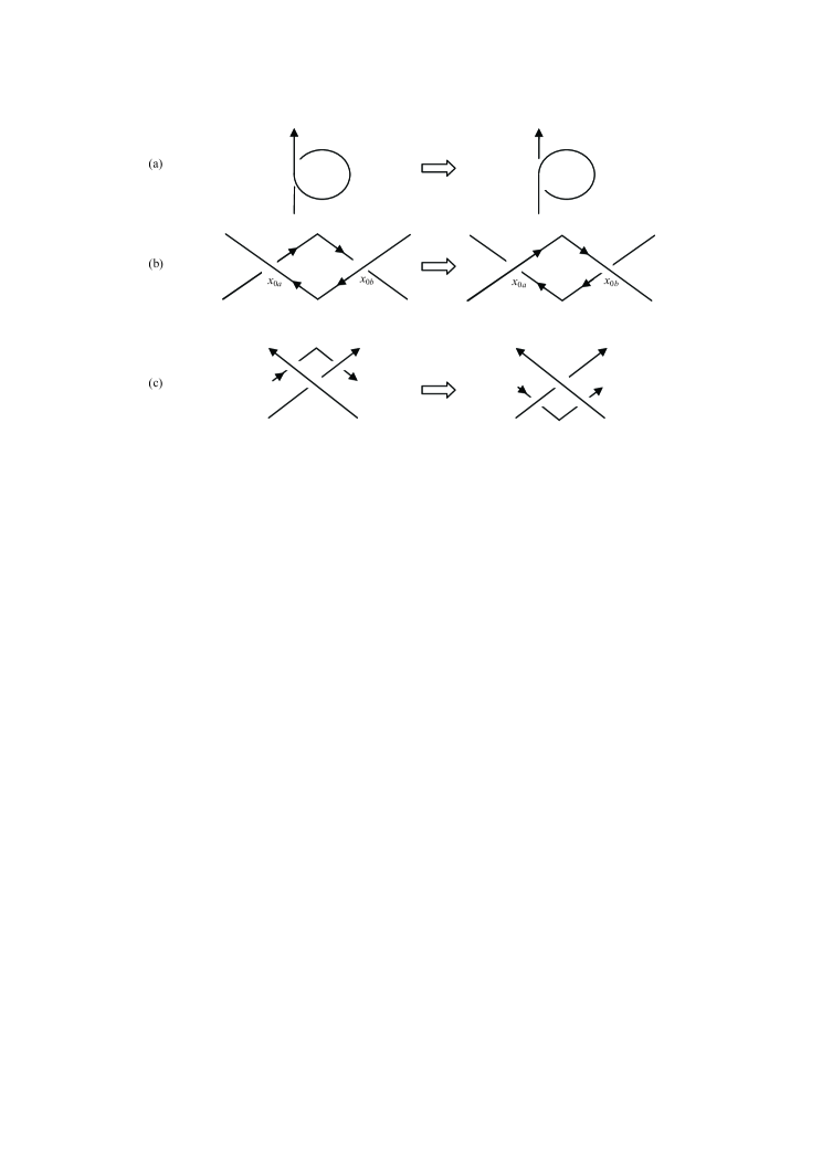
Figure 4: Reidemeister Moves: (a) Type-I; (b) Type-II; (c) Type-III.

In following the relationships between the $S_{L}\left(\alpha,\beta,z\right)$ polynomial and other knot polynomial invariants will be studied. $\left\langle W\left(L\right)\right\rangle$ will be modified to be an ambient-isotopic invariant, and a difference between the normal and super Lie gauge groups, $SU\left(N\right)$ and $SU\left(M|N\right)$, will arise from the Jones polynomial.

Firstly, the ambient-isotopic HOMFLY knot polynomial invariant can be constructed from $\left\langle W\left(L\right)\right\rangle$ by introducing a factor describing knot writhing:

$$\left\langle P\left(L\right)\right\rangle=\alpha^{-\omega\left(L\right)}\left\langle W\left(L\right)\right\rangle.$$ (44)

Here $\omega\left(L\right)$ is the writhe number of a knot $L$, defined as

$$\omega\left(L_{\pm}\right)=\omega\left(L_{0}\right)+\epsilon\left(L_{\pm};x_{0}\right)=\omega\left(L_{0}\right)\pm 1,$$ (45)

where $\epsilon\left(L_{\pm};x_{0}\right)$ is the sign of the crossing point $x_{0}$ on $L_{\pm}$: $\epsilon\left(L_{\pm};x_{0}\right)=\pm 1$. For $\hat{L}_{+},\ \hat{L}_{-}$ and $\hat{L}_{0}$, (45) reads

$$\omega\left(\hat{L}_{+}\right)=\omega\left(\hat{L}_{0}\right)+1,\ \ \ \ \omega\left(\hat{L}_{-}\right)=\omega\left(\hat{L}_{0}\right)-1.$$ (46)

(46) means that $\hat{L}_{+}$ contributes a $1$ to the writhe number, while $\hat{L}_{-}$ contributes a $\left(-1\right)$. Then using (39) and (44) one has

$$\left\langle P\left(\hat{L}_{+}\right)\right\rangle=\left\langle P\left(\hat{L}_{0}\right)\right\rangle,\ \ \ \ \left\langle P\left(\hat{L}_{-}\right)\right\rangle=\left\langle P\left(\hat{L}_{0}\right)\right\rangle,$$ (47)

meaning $\left\langle P\left(L\right)\right\rangle$ is invariant under the type-I Reidemeister move. Furthermore $\langle P\left(L\right)\rangle$ satisfies

$$\left(\alpha\beta\right)\left\langle P\left(L_{+}\right)\right\rangle-\left(\alpha\beta\right)^{-1}\left\langle P\left(L_{-}\right)\right\rangle=zP\left(L_{0}\right).$$ (48)

Hence one arrives at the skein relations for $\left\langle P\left(L\right)\right\rangle:$

$$\left\langle P\left(\hat{L}_{c}\right)\right\rangle=M-N,$$ (49)

$$t\left\langle P\left(L_{+}\right)\right\rangle-t^{-1}\left\langle P\left(L_{-}\right)\right\rangle=z\left\langle P\left(L_{0}\right)\right\rangle,$$ (50)

where

$$t\equiv\alpha\beta=1-i\frac{2\pi}{k}\frac{\left(M-N\right)}{2}+O\left(\frac{1}{k^{2}}\right),\ \ \ \ \ \ z=-i\frac{2\pi}{k}+O\left(\frac{1}{k^{2}}\right).$$ (51)

(49) can be obtained from (50) by considering $t\left\langle P\left(\tilde{L}_{+}\right)\right\rangle-t^{-1}\left\langle P\left(\tilde{L}_{-}\right)\right\rangle=z\left\langle P\left\langle\tilde{L}_{c}\right\rangle\right\rangle$, where $\tilde{L}_{+},\ \tilde{L}_{-}$ and $\tilde{L}_{c}$ denote unknots shown in Figure 5.

Figure 5: Unknots: (a) $\tilde{L}_{+}$; (b) $\tilde{L}_{-}$; (c) $\tilde{L}_{c}$.

Eqs.(49) and (50) show $\left\langle P\left(L\right)\right\rangle$ is an ambient-isotopic HOMFLY polynomial invariant.

Secondly, if specially $M-N=2$ in (49) to (51), the $z$ is related to $t$ as $z=t^{\frac{1}{2}}-t^{-\frac{1}{2}}$, up to the first order. This means that in the $SU\left(N+2|N\right)$ CS field theory, under the fundamental representation there is a knot polynomial $\left\langle V\left(L\right)\right\rangle\equiv\left\langle P\left(L\right)\right\rangle$ which satisfies the skein relation

$$t\left\langle V\left(L_{+}\right)\right\rangle-t^{-1}\left\langle V\left(L_{-}\right)\right\rangle=\left(t^{\frac{1}{2}}-t^{-\frac{1}{2}}\right)\left\langle V\left(L_{0}\right)\right\rangle.$$ (52)

This $\left\langle V\left(L\right)\right\rangle$ is known as the Jones polynomial . Therefore there are a series of CS theories with Lie super gauge group $SU\left(N+2|N\right),\ N\in\mathbb{Z}^{+},$ which have the Jones polynomial. This is different from the situation of the CS theory with normal Lie group $SU\left(N\right)$ — it is known that under the fundamental representation, only the $SU\left(2\right)$ theory has the Jones polynomial invariant among all $SU\left(N\right)$ CS theories, $\ N=2,3,\cdots\$ [3, 1, 8].

Different choices of gauge groups with different algebraic representations lead to different knot polynomials in CS field theories [8]. In our further work the relationship between the $S_{L}\left(\alpha,\beta,z\right)$ and the Kauffman polynomials in the $OSp\left(1|2\right)$ CS field theory will be studied.

Finally, the $\alpha,\ \beta$ and $z$ in the $S_{L}\left(\alpha,\beta,z\right)$ polynomial and the $t$ in the HOMFLY polynomial can be expressed in a unified way. Introducing a variable

$$q=e^{-i\frac{2\pi}{k}},$$ (53)

$\alpha,\ \beta$, $z$ and $t$ can be regarded as the lower order expansions of the $q$ exponentials [4, 1, 3]: $\alpha=q^{C_{2}}=q^{\frac{\left(M-N\right)^{2}-1}{2\left(M-N\right)}},\ \beta=q^{\frac{1}{2\left(M-N\right)}},\ z=q^{\frac{1}{2}}-q^{-\frac{1}{2}}$ and $t=q^{\frac{M-N}{2}}.$ Then the $S_{L}\left(\alpha,\beta,z\right)$ shown in (38)–(40) and HOMFLY polynomial in (49)–(50) can be written more elegantly as

$$\left\langle W\left(\hat{L}_{c}\right)\right\rangle=M-N\ \ \ \ \left(M\neq N\right),$$ (54)

$$\left\langle W\left(\hat{L}_{+}\right)\right\rangle=q^{\frac{\left(M-N\right)^{2}-1}{2\left(M-N\right)}}\left\langle W\left(\hat{L}_{0}\right)\right\rangle,$$ (55)

$$\left\langle W\left(\hat{L}_{-}\right)\right\rangle=q^{-\frac{\left(M-N\right)^{2}-1}{2\left(M-N\right)}}\left\langle W\left(\hat{L}_{0}\right)\right\rangle,$$ (56)

$$q^{\frac{1}{2\left(M-N\right)}}\left\langle W\left(L_{+}\right)\right\rangle-q^{-\frac{1}{2\left(M-N\right)}}\left\langle W\left(L_{-}\right)\right\rangle=\left(q^{\frac{1}{2}}-q^{-\frac{1}{2}}\right)\left\langle W\left(L_{0}\right)\right\rangle,$$ (57)

and

$$\left\langle P\left(\hat{L}_{c}\right)\right\rangle=\frac{q^{\frac{M-N}{2}}-q^{-\frac{M-N}{2}}}{q^{\frac{1}{2}}-q^{-\frac{1}{2}}},$$ (58)

$$q^{\frac{M-N}{2}}\left\langle P\left(L_{+}\right)\right\rangle-q^{-\frac{M-N}{2}}\left\langle P\left(L_{-}\right)\right\rangle=\left(q^{\frac{1}{2}}-q^{-\frac{1}{2}}\right)\left\langle P\left(L_{0}\right)\right\rangle.$$ (59)

5 Conclusion

In this paper we have studied knots in the CS field theory with gauge group $SU\left(M|N\right)$. In Section 2, the notation for the fundamental representation of the Lie superalgebra $\mathfrak{su}\left(M|N\right)$ is fixed, and an important property of the CS action, Eq.(12), is presented. In Section 3, variation of the correlation function of Wilson loops is rigorously studied. In Section 4, the variation of correlation functions (26) is discussed for different link configurations. It is addressed that the path integrals have been formally expressed as propagators instead of being integrated out. A rigorous development of techniques for path integrals awaits future advances in the mathematical theory of functional integrals. From the formal analysis the $S_{L}\left(\alpha,\beta,z\right)$ knot polynomial and its skein relations, (38) to (40), are obtained. In terms of the $S_{L}\left(\alpha,\beta,z\right)$ polynomial the HOMFLY and Jones knot polynomials as well as their skein relations (49) to (52) have been derived by considering the knot writhing.

6 Acknowledgment

The author is indebted to Prof. R.B. Zhang and Dr. W.L. Yang for instructive advices and warmhearted help. This work was financially supported by the USYD Postdoctoral Fellowship of the University of Sydney, Australia.

References

[1] Guadagnini, E.: The Link Invariants of the
Chern-Simons Field Theory, Walter de Gruyter & Co., Berlin, 1993.
[2] Deser, S., Jackiw, R., Templeton, S.: Ann. Phys.140 (1982) 372;
Jackiw, R.: Topological
Investigations of Quantized Gauge Theories, in Current
Algebras and Anomalies, edited by Treiman S.B., Jackiw R., Zumino
B. and Witten E., World Scientific, 1985.
[8] Labastida, J.M.F.: Chern-Simons Gauge Theory: Ten Years After, in
Trends in Theoretical Physics II, H. Falomir, R. Gamboa, F.
Schaposnik, eds., American Institute of Physics, New York, 1999, CP 484
(1-41), available at: hep-th/9905057.
[9] Marino, M., Rev. Mod. Phys.77
(2005) 675.
[10] Gambini, R., Pullin, J.: Loops, Knots,
Gauge Theories and Quantum Gravity, Cambridge, Cambridge
University Press, 1996;
Li, W., Song, W., Strominger, A.:
JHEP0804 (2008) 082.
[12] Scheunert, M., Nahm, W., Rittenberg, V.: J.
Math. Phys.18 (1977) 146.
[13] Gould, M., Zhang, R.: J. Math. Phys.31
(1990) 1524; ibid., J. Math. Phys.31 (1990) 2552.
Scheunert, M.; Zhang, R.: J. Algebra292 (2005) 324.
[14] Zhang, R., Gould, M., Bracken, A.: Commun.
Math. Phys.137 (1991) 13;
Kauffman, L.H., Saleur, H.: Commun. Math. Phys.141 (1991)
293;
Gould, M., Tsohantjis, I., Bracken, A.: Rev. Math. Phys.5
(1993) 533;
Links, J., Gould, M., Zhang, R.: Rev. Math. Phys.5 (1993)
345;
Links, J., Zhang, R.: J. Math. Phys.35 (1994) 1377.
[15] Bourdeau, M., et al.: Nucl. Phys. B372 (1992) 303;
Ennes, I.P., et al.: Int. J. Mod. Phys. A13 (1998) 2931;
Gaiotto, D., Witten, E.: Janus Configurations, Chern-Simons
Couplings, and the -Angle in Super Yang-Mills Theory, available at: arXiv:0804.2907 [hep-th].