Random recursive triangulations of the disk via fragmentation theory

Abstract

We introduce and study an infinite random triangulation of the unit disk that arises as the limit of several recursive models. This triangulation is generated by throwing chords uniformly at random in the unit disk and keeping only those chords that do not intersect the previous ones. After throwing infinitely many chords and taking the closure of the resulting set, one gets a random compact subset of the unit disk whose complement is a countable union of triangles. We show that this limiting random set has Hausdorff dimension $\beta^{*}+1$, where $\beta^{*}=(\sqrt{17}-3)/2$, and that it can be described as the geodesic lamination coded by a random continuous function which is Hölder continuous with exponent $\beta^{*}-\varepsilon$, for every $\varepsilon>0$. We also discuss recursive constructions of triangulations of the $n$-gon that give rise to the same continuous limit when $n$ tends to infinity.

and

1 Introduction

In this work, we use fragmentation theory to study an infinite random triangulation of the unit disk that arises as the limit of several recursive models. Let us describe a special case of these models in order to introduce our main object of interest. We consider a sequence $U_{1},V_{1},U_{2},\allowbreak V_{2},\ldots$ of independent random variables, which are uniformly distributed over the unit circle $\mathbb{S}_{1}$ of the complex plane. We then construct inductively a sequence $L_{1},L_{2},\ldots$ of random closed subsets of the (closed) unit disk $\overline{\mathbb{D}}$. To begin with, $L_{1}$ just consists of the chord with endpoints $U_{1}$, and $V_{1}$, which we denote by $[U_{1}V_{1}]$. Then at step $n+1$, we consider two cases. Either the chord $[U_{n+1}V_{n+1}]$ intersects $L_{n}$, and we put $L_{n+1}=L_{n}$, or the chord $[U_{n+1}V_{n+1}]$ does not intersect $L_{n}$, and we put $L_{n+1}=L_{n}\cup[U_{n+1}V_{n+1}]$. Thus, for every integer $n\geq 1$, $L_{n}$ is a disjoint union of random chords. We then let

$$L_{\infty}=\overline{\bigcup_{n=1}^{\infty}L_{n}}$$

be the closure of the (increasing) union of the sets $L_{n}$. See Figure 1 below for a simulation of the set $L_{\infty}$.

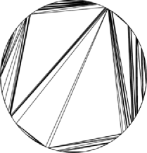
Figure 1: The random set $L_{\infty}$.

The closed set $L_{\infty}$ is a geodesic lamination of the unit disk, in the sense that it is a closed union of noncrossing chords (here we say that two chords do not cross if they do not intersect except possibly at their endpoints). We refer to Bon98 for the general notion of a geodesic lamination of a surface in the setting of hyperbolic geometry. We may also view $L_{\infty}$ as an infinite triangulation of the unit disk, in the same sense as in Aldous Ald94b . Precisely, $L_{\infty}$ is a closed subset of $\overline{\mathbb{D}}$, which has zero Lebesgue measure and is such that any connected component of $\overline{\mathbb{D}}\setminus L_{\infty}$ is a triangle whose vertices belong to the circle $\mathbb{S}_{1}$. The latter properties are not immediate, but will follow from forthcoming statements.

In order to state our first result, let us introduce some notation. We denote the number of chords in $L_{n}$ by $N(L_{n})$. Then, for every $x,y\!\in\!\mathbb{S}_{1}$, we let $H_{\!n}(x,y)$ be the number of chords in $L_{n}$ that intersect the chord $[xy]$. We also set

$$\beta^{*}=\frac{\sqrt{17}-3}{2}.$$

Theorem 1.1

(i) We have

$$n^{-1/2}N(L_{n})\stackrel{{\scriptstyle a.s.}}{{\mathop{\longrightarrow}\limits_{n\to\infty}}}\sqrt{\pi}.$$

(ii) There exists a random process $(\mathscr{M}_{\infty}(x),x\in\mathbb{S}_{1})$, which is Hölder continuous with exponent $\beta^{*}-\varepsilon$, for every $\varepsilon>0$, such that, for every $x\in\mathbb{S}_{1}$,

$$n^{-\beta^{*}/2}H_{n}(1,x)\stackrel{{\scriptstyle(\mathbb{P})}}{{\mathop{\longrightarrow}\limits_{n\to\infty}}}\mathscr{M}_{\infty}(x),$$

where $\stackrel{{\scriptstyle(\mathbb{P})}}{{\longrightarrow}}$ denotes convergence in probability.

Part (i) of the theorem is a rather simple consequence of the results in BD86 , BD87 , but part (ii) is more delicate and requires different tools. In the present work, we prove (more general versions of) the convergences in (i) and (ii) by using fragmentation theory. To this end, we consider continuous-time models where noncrossing chords are thrown at random in the unit disk according to the following device: At time $t$, the existing chords bound several subdomains of the disk, and a new chord is created in one of these subdomains at a rate which is a given power of the Lebesgue measure of the portion of the circle that is adjacent to this subdomain. It is not hard to see that the random closed subset of $\overline{\mathbb{D}}$ obtained by taking the closure of all chords created in this process has the same distribution as $L_{\infty}$, and moreover the case when the power is the square is very closely related to the discrete-time model described above.

In this continuous-time model, the ranked sequence of the Lebesgue measures of the portions of $\mathbb{S}_{1}$ corresponding to the subdomains bounded by the existing chords at time $t$ forms a conservative fragmentation process, in the sense of Ber06 . A general version of the convergence (i) can then be obtained as a consequence of asymptotics for fragmentation processes. Similarly, if $U$ is a random point uniformly distributed on $\mathbb{S}_{1}$ and if we look only at subdomains that intersect the chord $[1U]$, we get another (dissipative) fragmentation process, and known asymptotics give the convergence in (ii), provided that $x$ is replaced by the random point $U$. An extra absolute continuity argument is then needed to get the desired result for a deterministic point $x$: See Theorem 3.13 and its proof. It is plausible that the convergence in (ii) also holds almost surely, but the known asymptotics for fragmentation processes do not give this stronger form.

The most technical part of the proof of Theorem 1.1 is the derivation of the Hölder continuity properties of the limiting process $(\mathscr{M}_{\infty}(x),x\in\mathbb{S}_{1})$. To this end, we need to obtain precise bounds for the moments of increments of this process. In order to derive these bounds, we rely on integral equations for the moments, which follow from the recursive construction.

Our second theorem shows that the random geodesic lamination $L_{\infty}$ is coded by the process $\mathscr{M}_{\infty}$, in the sense of the following statement. For every $x,y\in\mathbb{S}_{1}\setminus\{1\}$, we let $\operatorname{Arc}(1,x)=\operatorname{Arc}(x,1)$ be the closed subarc of $\mathbb{S}_{1}$ with endpoints $x$ and $y$ that does not contain the point $1$. For every $x\in\mathbb{S}_{1}\setminus\{1\}$, we let $\operatorname{Arc}(1,x)=\operatorname{Arc}(x,1)$ be the closed subarc of $\mathbb{S}_{1}$ going from $1$ to $x$ in counterclockwise order, and we set $\operatorname{Arc}(1,1)=\{1\}$ by convention.

Theorem 1.2

The following properties hold almost surely. The random set $L_{\infty}$ is the union of the chords $[xy]$ for all $x,y\in\mathbb{S}_{1}$ such that

$$\mathscr{M}_{\infty}(x)=\mathscr{M}_{\infty}(y)=\min_{z\in\operatorname{Arc}(x,y)}\mathscr{M}_{\infty}(z).$$ (1)

Moreover, $L_{\infty}$ is maximal for the inclusion relation among geodesic laminations.

It is relatively easy to see that property (1) holds for any chord $[xy]$ that arises in our construction of $L_{\infty}$. The difficult part of the proof of the theorem is to show the converse, namely that any chord $[xy]$ such that (1) holds will be contained in $L_{\infty}$. This fact is indeed closely related to the maximality property of $L_{\infty}$.

The coding of geodesic laminations by continuous functions is discussed in LGP08 , and is closely related to the coding of $\mathbb{R}$-trees by continuous functions (see, e.g., DLG05 ). A particular instance of this coding had been discussed earlier by Aldous Ald94b , who considered the case when the coding function is the normalized Brownian excursion. In that case, the associated $\mathbb{R}$-tree is Aldous’s CRT. Moreover, the Hausdorff dimension of the corresponding lamination is $3/2$. This may be compared to the following statement, where $\operatorname{dim}(A)$ stands for the Hausdorff dimension of a subset $A$ of the plane.

Theorem 1.3

We have almost surely

$$\operatorname{dim}(L_{\infty})=\beta^{*}+1=\frac{\sqrt{17}-1}{2}.$$

The lower bound $\operatorname{dim}(L_{\infty})\geq\beta^{*}+1$ is a relatively easy consequence of the fact that $L_{\infty}$ is coded by the function ${\mathscr{M}}_{\infty}$ (Theorem 1.2) and of the Hölder continuity properties of this function (Theorem 1.1). In order to get the corresponding upper bound, we use explicit coverings of the set $L_{\infty}$ that follow from our recursive construction. To evaluate the sum of the diameters of balls in these coverings raised to a suitable power, we again use certain asymptotics from fragmentation theory.

The random set $L_{\infty}$ also occurs as the limit in distribution of certain random recursive triangulations of the $n$-gon. For every $n\geq 3$, we consider the $n$-gon whose vertices are the $n$th roots of unity

$$x^{n}_{k}=\exp\biggl{(}2i\pi\frac{k}{n}\biggr{)},\qquad k=1,2,\ldots,n.$$

A chord of $\mathbb{S}_{1}$ is called a diagonal of the $n$-gon if its vertices belong to the set $\{x^{n}_{k}\dvtx 1\leq k\leq n\}$ and if it is not an edge of the $n$-gon. A triangulation of the $n$-gon is the union of $n-3$ noncrossing diagonals of the $n$-gon (then the connected components of the complement of this union in the $n$-gon are indeed triangles). The set $\mathscr{T}_{n}$ of all triangulations of the $n$-gon is in one-to-one correspondence with the set of all planar binary trees with $n-1$ leaves (see, e.g., Aldous Ald94b ).

For every fixed integer $n\geq 4$, we construct a random element of $\mathscr{T}_{n}$ as follows. Denote by $\mathscr{D}_{n}$ the set of all diagonals of the $n$-gon. Let $c_{1}$ be chosen uniformly at random in $\mathscr{D}_{n}$. Then, conditionally given $c_{1}$, let $c_{2}$ be a chord chosen uniformly at random in the set of all chords in $\mathscr{D}_{n}$ that do not cross $c_{1}$. We continue by induction and construct a finite sequence of chords $c_{1},c_{2},\ldots,\allowbreak c_{n-3}$: for every $1<k\leq n-3$, $c_{k}$ is chosen uniformly at random in the set of all chords in $\mathscr{D}_{n}$ that do not cross $c_{1},c_{2},\ldots,c_{k-1}$. Finally we let $\Lambda_{n}$ be the union of the chords $c_{1},c_{2},\ldots,c_{n-3}$.

Let us also introduce a slightly different model, which is closely related to DHW08 . Let $\sigma$ be a uniformly distributed random permutation of $\{1,2,\ldots,n\}$. With $\sigma$, we associate a collection of diagonals of the $n$-gon, which is constructed recursively as follows. For every integer $0\leq k\leq n$ we define a set $M_{k}$ of disjoint diagonals of the $n$-gon, and a set $F_{k}$ of “free” vertices. We start with $M_{0}=F_{0}=\varnothing$. Then, at step $k\in\{1,\ldots,n\}$, either there is a (necessarily unique) free vertex $x\in F_{k-1}$ such that $[xx^{n}_{\sigma(k)}]$ is a diagonal of the $n$-gon that does not intersect the chords in $M_{k-1}$, and we set $M_{k}=M_{k-1}\cup\{[xx^{n}_{\sigma(k)}]\}$ and $F_{k}=F_{k-1}\setminus\{x\}$; or there is no such vertex and we set $M_{k}=M_{k-1}$ and $F_{k}=F_{k-1}\cup\{x^{n}_{\sigma(k)}\}$. We let $\widetilde{\Lambda}_{n}$ be the union of the chords in $M_{n}$ (note that $\widetilde{\Lambda}_{n}$ is not a triangulation of the $n$-gon).

Theorem 1.4

We have

$$\Lambda_{n}\stackrel{{\scriptstyle(d)}}{{\mathop{\longrightarrow}\limits_{n\to\infty}}}L_{\infty}$$

and

$$\widetilde{\Lambda}_{n}\stackrel{{\scriptstyle(d)}}{{\mathop{\longrightarrow}\limits_{n\to\infty}}}L_{\infty}.$$

In both cases, the convergence holds in distribution in the sense of the Hausdorff distance between compact subsets of $\overline{\mathbb{D}}$.

Theorem 1.4 should be compared with the results of Aldous Ald94b (see also Ald94a ). Aldous considers a triangulation of the $n$-gon that is uniformly distributed over $\mathscr{T}_{n}$, and then proves that this random triangulation converges in distribution as $n\to\infty$ toward the geodesic lamination coded by the normalized Brownian excursion (see Theorem 2.6 below for a more precise statement). Our random recursive constructions give rise to a limiting geodesic lamination which is “bigger” than the one that appears in Aldous’s work, in the sense of Hausdorff dimension.

Triangulations of convex polygons are also interesting from the geometric and combinatorial point of view (see, e.g., STT88 ). In DFHN99 , Devroye et al. study some features of triangulations sampled uniformly from $\mathscr{T}_{n}$. Their proofs are based on combinatorial and enumeration techniques. Recursive triangulations of the type studied in the present work have been used in physics as greedy algorithms for computing folding of RNA structure (see Mul03 ). In these models, the polymer is represented by a discrete cycle and diagonals correspond to liaisons of RNA bases. See Mul03 , DHW08 , DDJS09 for certain results related to our work, and in particular to the asymptotics of Theorem 1.1.

As a final remark, this work deals with “Euclidean” geodesic laminations consisting of unions of chords. As in LGP08 , we may consider instead the hyperbolic geodesic laminations obtained by replacing each chord by the hyperbolic line with the same endpoints in the hyperbolic disk. It is immediate to verify that our main results remain valid after this replacement.

The paper is organized as follows. Section 2 recalls basic facts about geodesic laminations, and introduces the random processes $(S_{\alpha}(t))_{t\geq 0}$ describing random recursive laminations, which are of interest in this work. Section 3 studies the connections between these random processes and fragmentation theory, and derives general forms of the asymptotics of Theorem 1.1. Section 4 is devoted to the continuity properties of the process $\mathscr{M}_{\infty}$. Theorem 1.2 characterizing $L_{\infty}$ as the lamination coded by $\mathscr{M}_{\infty}$ is proved in Section 5. The Hausdorff dimension of $L_{\infty}$ is computed in Section 6, and Section 7 discusses the discrete models of Theorem 1.4. Finally, Section 8 gives some extensions and comments.

2 Random geodesic laminations

2.1 Laminations

Let us briefly recall the notation which was already introduced in Section 1. The open unit disk of the complex plane $\mathbb{C}$ is denoted by $\mathbb{D}=\{z\in\mathbb{C}\dvtx|z|<1\}$, and $\mathbb{S}_{1}$ is the unit circle. As usual, the closed unit disk is denoted by $\overline{\mathbb{D}}$. If $x,y$ are two distinct points of $\mathbb{S}_{1}$, the chord of feet $x$ and $y$ is the closed line segment $[xy]\subset\overline{\mathbb{D}}$. We also use the notation $]xy[$ for the open line segment with endpoints $x$ and $y$. By convention, $[xx]$ is equal to the singleton $\{x\}$, and is viewed as a degenerate chord, with $]xx[=\varnothing$.

We say that two chords $[xy]$ and $[x^{\prime}y^{\prime}]$ do not cross if $]xy[\,\cap\,]x^{\prime}y^{\prime}[\,=\varnothing$.

Definition 2.1.

A geodesic lamination $L$ of $\overline{\mathbb{D}}$ is a closed subset $L$ of $\overline{\mathbb{D}}$ which can be written as the union of a collection of noncrossing chords. The lamination $L$ is maximal if it is maximal for the inclusion relation among geodesic laminations of $\overline{\mathbb{D}}$.

For simplicity, we will often say lamination instead of geodesic lamination of $\overline{\mathbb{D}}$. In the context of hyperbolic geometry Bon98 , geodesic laminations of the disk are defined as closed subsets of the open (hyperbolic) disk. Here we prefer to view them as compact subsets of the closed disk, mainly because we want to discuss convergence of laminations in the sense of the Hausdorff distance. Notice that a maximal lamination necessarily contains the unit circle $\mathbb{S}_{1}$.

As the next lemma shows, the concept of a maximal lamination is a continuous analogue of a discrete triangulation.

Lemma 2.2

Let $L$ be a geodesic lamination of $\overline{\mathbb{D}}$. Then $L$ is maximal if and only if the connected components of $\overline{\mathbb{D}}\setminus L$ are open triangles whose vertices belong to $\mathbb{S}_{1}$.

We leave the easy proof to the reader.

2.2 Figelas and associated trees

The simplest examples of laminations are finite unions of noncrossing chords. Define a figela $S$ (from finite geodesic lamination) as a finite set of (unordered) pairs of distinct points of $\mathbb{S}_{1}$

$$S=\{\{x_{1},y_{1}\},\ldots,\{x_{n},y_{n}\}\},$$

such that the union of the $n$ chords $\{[x_{i}y_{i}]\}_{1\leq i\leq n}$ forms a lamination, which is then denoted by $L_{S}$. If $\{x,y\}\,{\in}\,S$, we will say that $[xy]$ is a chord of the figela $S$. We denote the set $\bigcup_{i=1}^{n}\{x_{i},y_{i}\}$ of all feet of the chords of $S$ by $\operatorname{Feet}(S)$.

Let $u,v\in\mathbb{S}_{1}\setminus\operatorname{Feet}(S)$. The height between $u$ and $v$ in $S$ is the number of chords of $S$ crossed by the chord $[uv]$

$$H_{S}(u,v)=\#\{1\leq i\leq n\dvtx[x_{i}y_{i}]\cap[uv]\neq\varnothing\}.$$

The next proposition follows from simple geometric considerations.

Proposition 2.3 ((Triangle inequality))

Let $S$ be a figela. For every $x,y,z\in\mathbb{S}_{1}\setminus\operatorname{Feet}(S)$ we have

$$H_{S}({x},{z})\leq H_{S}({x},{y})+H_{S}({y},{z}).$$ (2)

Let $S=\{\{x_{1},y_{1}\},\ldots,\{x_{n},y_{n}\}\}$ be a figela. We define an equivalence relation on $\mathbb{S}_{1}\setminus\operatorname{Feet}(S)$ by setting, for every $u,v\in\mathbb{S}_{1}\setminus\mbox{Feet}(S)$,

$$u\simeq v\quad\mbox{if and only if}\quad H_{S}(u,v)=0.$$

In other words, two points of $\mathbb{S}_{1}\setminus\operatorname{Feet}(S)$ are equivalent if and only if they belong to the same connected component of $\overline{\mathbb{D}}\setminus\bigcup_{i=1}^{n}[x_{i}y_{i}]$. Then $H_{S}$ induces a distance on the quotient set ${\mathcal{T}}_{S}:=(\mathbb{S}_{1}\setminus\operatorname{Feet}(S))/\!\!\simeq$. The finite metric space ${\mathcal{T}}_{S}$ can be viewed as a graph by declaring that there is an edge between $a$ and $b$ if and only if $H_{S}(a,b)=1$. This graph is indeed a tree, and $H_{S}(\cdot,\cdot)$ coincides with the usual graph distance. The tree ${\mathcal{T}}_{S}$ can be rooted at the equivalence class of $1$ (we assume that $1$ is not a foot of $S$, which will always be the case in our examples). As a result of this discussion, we can associate a plane (rooted ordered) tree ${\mathcal{T}}_{S}$ to $S$. See Figure 2 for an example from which the definition of the tree ${\mathcal{T}}_{S}$ should be clear.

The $n+1$ connected components of $\overline{\mathbb{D}}\setminus\bigcup_{i=1}^{n}[x_{i}y_{i}]$ are called the fragments of the figela $S$. With each fragment $R$, we associate its mass

$$\mathrm{m}(R)=\lambda(R\cap\mathbb{S}_{1}),$$

where $\lambda$ denotes the uniform probability measure on $\mathbb{S}_{1}$.

Figure 2: A figela and its associated plane tree (in dotted lines on the left side). We drew chords as curved lines for better visibility. In this example, $S$ has $7$ chords and $8$ fragments. Notice that each fragment of $S$ corresponds to a vertex of the tree ${\mathcal{T}}_{S}$.

2.3 Coding by continuous functions

Let $g\dvtx[0,1]\to\mathbb{R}_{+}$ be a continuous function such that $g(0)=g(1)=0$. We define a pseudo-distance on $[0,1]$ by

$$\mathrm{d}_{g}(s,t)=g(s)+g(t)-2\min_{r\in[s\wedge t,s\vee t]}g(r)$$

for every $s,t\in[0,1]$. The associated equivalence relation on $[0,1]$ is defined by setting $s\stackrel{{\scriptstyle g}}{{\sim}}t$ if and only if $\mathrm{d}_{g}(s,t)=0$, or equivalently $g(s)=g(t)=\min_{r\in[s\wedge t,s\vee t]}g(r)$.

Proposition 2.4 ((DLG05 ))

The quotient set $T_{g}:=[0,1]/\!\!\stackrel{{\scriptstyle g}}{{\sim}}$ endowed with the distance $\mathrm{d}_{g}$ is an $\mathbb{R}$-tree called the tree coded by the function $g$.

We refer to Eva08 for an extensive discussion of $\mathbb{R}$-trees in probability theory.

In order to introduce the lamination coded by $g$, we need some additional notation. For $s\in[0,1]$, we let $\operatorname{cl}_{g}(s)$ be the equivalence class of $s$ with respect to the equivalence relation $\stackrel{{\scriptstyle g}}{{\sim}}$. Then, for $s,t\in[0,1]$, we set $s\stackrel{{\scriptstyle g}}{{\approx}}t$ if at least one of the following two conditions holds:

• $s\stackrel{{\scriptstyle g}}{{\sim}}t$ and $g(r)>g(s)$ for every $r\in\,]s\wedge t,s\vee t[$.

• $s\stackrel{{\scriptstyle g}}{{\sim}}t$ and $s\wedge t=\min\operatorname{cl}_{g}(s)$, $s\vee t=\max\operatorname{cl}_{g}(s)$.

In particular, $s\stackrel{{\scriptstyle g}}{{\approx}}s$, and $s\stackrel{{\scriptstyle g}}{{\approx}}t$ holds if and only if $t\stackrel{{\scriptstyle g}}{{\approx}}s$. Note, however, that $\stackrel{{\scriptstyle g}}{{\approx}}$ is in general not an equivalence relation. It is an elementary exercise to check that the graph $\{(s,t)\dvtx s\stackrel{{\scriptstyle g}}{{\approx}}t\}$ is a closed subset of $[0,1]^{2}$.

Proposition 2.5

The set

$$L_{g}:=\bigcup_{s\stackrel{{\scriptstyle g}}{{\approx}}t}[e^{2i\pi s}e^{2i\pi t}]$$ (3)

is a geodesic lamination of $\overline{\mathbb{D}}$ called the lamination coded by the function $g$. Furthermore, $L_{g}$ is maximal if and only if, for every open subinterval $]s,t[$ of $[0,1]$, the infimum of $g$ over $]s,t[$ is attained at at most one point of $]s,t[$.

We leave the proof to the reader. See LGP08 , Proposition 2.1, for a closely related statement. This proposition is stated under the assumption that the local minima of $g$ are distinct, which is slightly stronger than the condition in the second assertion of Proposition 2.5. Note that the latter condition is equivalent to saying that the relations $\stackrel{{\scriptstyle g}}{{\sim}}$ and $\stackrel{{\scriptstyle g}}{{\approx}}$ coincide, or that $\stackrel{{\scriptstyle g}}{{\approx}}$ is an equivalence relation.

We end this section by reformulating in this formalism a theorem of Aldous which was already mentioned in Section 1. Recall our notation $\mathscr{T}_{n}$ for the set of all triangulations of the $n$-gon. An element of $\mathscr{T}_{n}$ is just a geodesic lamination consisting of $n-3$ chords whose feet belong to the set of $n$th roots of unity.

Theorem 2.6 ((Ald94b , Ald94a ))

Let $(\mathbf{e}_{t})_{0\leq t\leq 1}$ be a normalized Brownian excursion, and let $\Delta_{n}$ be uniformly distributed over $\mathscr{T}_{n}$. Then we have

$$\Delta_{n}\stackrel{{\scriptstyle(d)}}{{\mathop{\longrightarrow}\limits_{n\to\infty}}}L_{\mathbf{e}},$$

in the sense of the Hausdorff distance between compact subsets of $\mathbb{\overline{D}}$. Moreover the Hausdorff dimension of $L_{\mathbf{e}}$ is almost surely equal to $3/2$.

A detailed argument for the calculation of the Hausdorff dimension of $L_{\mathbf{e}}$ is given in LGP08 (the proof in Ald94b is only sketched).

2.4 Random recursive laminations

Let $\alpha\geq 0$ be a positive real number. We define a Markov jump process $(S_{\alpha}(t),t\geq 0)$ taking values in the space of all figelas, and increasing in the sense of the inclusion order.

Let us describe the construction of this process. We introduce a sequence of random times $0=\tau_{0}<\tau_{1}<\tau_{2}<\cdots$ such that $S_{\alpha}(t)$ is constant over each interval $[\tau_{n},\tau_{n+1}[$, and $S_{\alpha}(\tau_{n})$ has exactly $n$ chords [in particular $S_{\alpha}(0)$ is the empty figela]. We define the pairs $(\tau_{n},S_{\alpha}(\tau_{n}))$ for every $n\geq 1$ recursively as follows. In order to describe the joint distribution of $(\tau_{n+1},S_{\alpha}(\tau_{n+1}))$ given the $\sigma$-field $\mathcal{F}_{n}=\sigma(\tau_{0},\ldots,\tau_{n},S_{\alpha}(\tau_{1}),\ldots,S_{\alpha}(\tau_{n}))$, we write $R_{1}^{n},\ldots,R_{n+1}^{n}$ for the $n+1$ fragments of the figela $S_{\alpha}(\tau_{n})$, and we let ${e}_{1},\ldots,{e}_{n+1}$ be $n+1$ independent exponential variables with parameter $1$ that are also independent of $\mathcal{F}_{n}$. Then, for $1\leq j\leq n+1$, we set $\mathcal{E}_{j}=\mathrm{m}(R_{j}^{n})^{-\alpha}{e}_{j}$ and we let $j_{0}$ be the a.s. unique index such that $\mathcal{E}_{j_{0}}=\min\{\mathcal{E}_{j}\dvtx 1\leq j\leq n+1\}$. Conditionally given $\mathcal{F}_{n}$ and $({e}_{1},\ldots,{e}_{n})$, we sample two independent random variables $X_{n+1},$ and $Y_{n+1}$ uniformly distributed over $R_{j_{0}}\cap\mathbb{S}_{1}$. Then conditionally on $\mathcal{F}_{n}$, the pair $(\tau_{n+1},S_{\alpha}(\tau_{n+1}))$ has the same distribution as $(\tau_{n}+\mathcal{E}_{j_{0}},S_{\alpha}(\tau_{n})\cup\{\{X_{n+1},Y_{n+1}\}\})$.

Note that $\tau_{n}\to\infty$ a.s. when $n\to\infty$. Indeed, it is enough to see this when $\alpha=0$, and then $\tau_{n+1}-\tau_{n}$ is exponential with parameter $n+1$. Therefore the processes $S_{\alpha}(t)$ are well-defined for every $t\geq 0$.

If $R$ is a fragment of $S_{\alpha}(t)$, then independently of the past up to time $t$, a new chord is added in $R$ at rate $\mathrm{m}(R)^{\alpha}$. The preceding construction can thus be interpreted informally: the first chord is thrown in $\overline{\mathbb{D}}$ uniformly at random (the two endpoints of the chord are chosen independently and uniformly over $\mathbb{S}_{1}$) at an exponential time with parameter $1$, and divides it into two fragments $R_{0}$ and $R_{1}$. These two fragments can be identified with two disks if we contract the first chord (the boundaries of these disks are then identified, respectively, with $R_{i}\cap\mathbb{S}_{1}$ for $i\in\{0,1\}$). Then the process goes on independently inside each of these disks provided that we rescale time by the mass of the corresponding fragment to the power $\alpha$.

The process $(S_{\alpha}(t),t\geq 0)$ will be called the figela process with autosimilarity parameter $\alpha$.

Remark 2.7.

Let $\{(t_{i},(x_{i},y_{i}))\}_{i\in\mathbb{N}}$ be the atoms of a Poisson point measure on $\mathbb{R}_{+}\times\mathbb{S}_{1}\times\mathbb{S}_{1}$ with intensity $dt\otimes\lambda\otimes\lambda$, where we recall that $\lambda$ is the uniform probability measure on $\mathbb{S}_{1}$. We suppose that the atoms of the Poisson measure are ordered so that $0<t_{1}<t_{2}<\cdots,$ and we also set $t_{0}=0$. We construct a figela-valued jump process $(\mathscr{S}(t),t\geq 0)$ using the following device. We start from $\mathscr{S}(0)=\varnothing$, and the process may jump only at times $t_{1},t_{2},\ldots.$ For every $i\geq 1$, we take $\mathscr{S}(t_{i})=\mathscr{S}(t_{i-1})\cup\{\{x_{i},y_{i}\}\}$ if the chord of feet $x_{i}$ and $y_{i}$ does not cross any chord of $\mathscr{S}(t_{i-1})$, and otherwise we take $\mathscr{S}(t_{i})=\mathscr{S}(t_{i-1})$. It follows from properties of Poisson measures that this process has the same law as our process $(S_{2}(t),t\geq 0)$. Moreover, the discrete-time process $(L_{\mathscr{S}(t_{n})},n\geq 0)$ has the same distribution as the process $(L_{n},n\geq 0)$ discussed in Section 1. Thanks to this observation, and to the fact that $n^{-1}t_{n}$ tends to $1$ a.s., forthcoming results about asymptotics of the processes $(S_{\alpha}(t),t\geq 0)$ will carry over to the process $(L_{n},n\geq 0)$.

Remark 2.8 ((Rotational invariance)).

Let $(S_{\alpha}(t))_{t\geq 0}$ be a figela process with parameter $\alpha$. For every $z\in\mathbb{S}_{1}$, set

$${S}^{z}_{\alpha}(t)=\bigl{\{}\{zx,zy\}\dvtx\{x,y\}\in S_{\alpha}(t)\bigr{\}}.$$

Then $({S}^{z}_{\alpha}(t),t\geq 0)$ has the same distribution as $({S}_{\alpha}(t),t\geq 0)$.

It will be important to construct simultaneously the processes $(S_{\alpha}(t))_{t\geq 0}$ for all values of $\alpha\geq 0$, in the following way. We set

$${\mathbb{T}}=\bigcup_{n\geq 0}\{0,1\}^{n},$$ (4)

where $\{0,1\}^{0}=\{\varnothing\}$. We consider a collection $(\epsilon_{u})_{u\in{\mathbb{T}}}$ of independent exponential variables with parameter $1$. The first chord then appears at time $\epsilon_{\varnothing}$. If $R_{0}$ and $R_{1}$ are the two fragments created at this moment, a new chord will appear in $R_{0}$, respectively, in $R_{1}$, at time $\epsilon_{\varnothing}+\mathrm{m}(R_{0})^{-\alpha}\epsilon_{0}$, respectively, at time $\epsilon_{\varnothing}+\mathrm{m}(R_{1})^{-\alpha}\epsilon_{1}$. We continue the construction by induction. If we use the same random choices of the new chords independently of $\alpha$ (so that the same fragments will also appear), we get a coupling of the processes $(S_{\alpha}(t))_{t\geq 0}$ for all $\alpha\geq 0$.

This coupling is such that a.s. for every $t\geq 0$ and for every $\alpha^{\prime}\geq\alpha\geq 0$, there exists a finite random time $T_{t,\alpha,\alpha^{\prime}}\geq t$ such that

$$S_{\alpha^{\prime}}(t)\subset S_{\alpha}(t)\subset S_{\alpha^{\prime}}(T_{t,\alpha,\alpha^{\prime}}).$$

In the remaining part of this work, we will always assume that the processes $(S_{\alpha}(t))_{t\geq 0}$ are coupled in this way. Hence, the increasing limit $S(\infty)=\lim\uparrow S_{\alpha}(t)$ as $t\uparrow\infty$ does not depend on $\alpha$, and the same holds for the random closed subset of $\overline{\mathbb{D}}$ defined by

$$L_{\infty}=\overline{\bigcup_{\{x,y\}\in S(\infty)}[xy]}.$$

By the discussion in Remark 2.7, this is consistent with the definition of $L_{\infty}$ in Section 1. We note that $L_{\infty}$ is a (random) geodesic lamination. To see this, write $S^{*}(\infty)$ for the closure in $\mathbb{S}_{1}\times\mathbb{S}_{1}$ of the set of all (ordered) pairs $(x,y)$ such that $\{x,y\}$ belongs to $S(\infty)$. Then a simple argument shows that

$$L_{\infty}=\bigcup_{(x,y)\in S^{*}(\infty)}[xy],$$

and moreover if $(x,y)$ and $(x^{\prime},y^{\prime})$ belong to $S^{*}(\infty)$ the chords $[xy]$ and $[x^{\prime}y^{\prime}]$ either coincide or do not cross.

3 Random fragmentations

3.1 Fragmentation theory

In this subsection, we briefly recall the results from fragmentation theory that we will use, in the particular case of binary fragmentation which is relevant to our applications. For a more detailed presentation, we refer to Bertoin’s book Ber06 .

We consider a probability measure $\nu$ on $[0,1]^{2}$. We assume that $\nu$ is supported on the set $\{(s_{1},s_{2})\dvtx 1>s_{1}\geq s_{2}\geq 0,s_{1}+s_{2}\leq 1\}$, and satisfies the following additional properties:

$$\mbox{(i)}\quad\nu(\{s_{2}>0\})>0.$$

(H)

$$\mbox{(ii)}\quad\nu(\{s_{1}=0\})=0.$$

Such a measure is a special case of a dislocation measure. Furthermore, if $\nu(\{s_{1}+s_{2}=1\})=1$, then $\nu$ is said to be conservative. It is called nonconservative or dissipative otherwise.

Let $\mathcal{S}^{\downarrow}$ be the set of all real sequences $(s_{1},s_{2},\ldots)$ such that $1\geq s_{1}\geq s_{2}\geq\cdots\geq 0$ and $\sum_{i=1}^{\infty}s_{i}\leq 1$. A fragmentation process with autosimilary parameter $\alpha\geq 0$, and dislocation measure $\nu$ is a Markov process $(X^{(\alpha)}(t),t\geq 0)$ with values in $\mathcal{S}^{\downarrow}$ whose evolution can be described informally as follows (see Ber06 for a more rigorous presentation). Let $X^{(\alpha)}(t)=(s_{1}(t),s_{2}(t),\ldots)$ be the state of the process at time $t\geq 0$. For each $i\geq 1$, $s_{i}(t)$ represents the mass of the $i$th particle at time $t$ (particles are ranked according to decreasing masses). Conditionally on the past up to time $t$, the $i$th particle lives after time $t$ during an exponential time of parameter $(s_{i}(t))^{\alpha}$, then dies and gives birth to two particles of respective masses $R_{1}s_{i}(t)$ and $R_{2}s_{i}(t)$, where the pair $(R_{1},R_{2})$ is sampled from $\nu$ independently of the past.

Remark 3.1.

We will not be interested in the case $\alpha<0$, which is not relevant for our applications.

We can construct simultaneously the processes $(X^{(\alpha)}(t))_{t\geq 0}$ starting from $X^{(\alpha)}(0)=(1,0,\ldots)$, for all values of $\alpha\geq 0$ in the following way. Consider first the process $X^{(0)}$ corresponding to $\alpha=0$. We represent the genealogy of this process by the infinite binary tree $\mathbb{T}$ defined in (4). Each $u\in{\mathbb{T}}$ thus corresponds to a “particle” in the fragmentation process. We denote the mass of $u$ by $\xi_{u}$ and the lifetime of $u$ by $\zeta^{(0)}_{u}$. Since we are considering the case $\alpha=0$, the random variables $(\zeta^{(0)}_{u})_{u\in\mathbb{T}}$ are independent and exponentially distributed with parameter $1$. If we now want to construct $(X^{(\alpha)}(t))_{t\geq 0}$ for a given value of $\alpha$, we keep the same values $\xi_{u}$ for the masses of particles, but we replace the lifetimes by $\zeta^{(\alpha)}_{u}=(\xi_{u})^{-\alpha}\zeta^{(0)}_{u}$, for every $u\in\mathbb{T}$. See Ber06 , Corollary 1.2, for more details.

In the remaining part of this subsection, we assume that the processes $(X^{(\alpha)}(t))_{t\geq 0}$ starting from $X^{(\alpha)}(0)=(1,0,\ldots)$ are defined for every $\alpha\geq 0$ and coupled as explained above.

We set for every real $p\geq 0$,

$$\kappa_{\nu}(p)=\int_{[0,1]^{2}}\bigl{(}1-(s_{1}^{p}+s_{2}^{p})\bigr{)}\nu(ds_{1},ds_{2}),$$

where by convention $0^{0}=0$. Then $\kappa_{\nu}$ is a continuous increasing function. Under Assumption $(H)$, $\kappa_{\nu}(0)<0$ and $\kappa_{\nu}(+\infty)=1$, and therefore there exists a unique $p^{*}>0$, called the Malthusian exponent of $\nu$, such that

$$\kappa_{\nu}(p^{*})=0.$$

The Malthusian exponent allows us to introduce the so-called Malthusian martingale, which is discussed in part (i) of the next theorem.

Theorem 3.2

Write $X^{(\alpha)}(t)=(s_{1}^{(\alpha)}(t),s_{2}^{(\alpha)}(t),\ldots)$ for every $t\geq 0$ and $\alpha\geq 0$. Then: [(iii)]

For every $\alpha\geq 0$, the process

$$\mathscr{M}^{(\alpha)}(t):=\sum_{i=1}^{\infty}\bigl{(}s_{i}^{(\alpha)}(t)\bigr{)}^{p^{*}},\qquad t\geq 0,$$

is a uniformly integrable martingale and converges almost surely to a limiting random variable $\mathscr{M}_{\infty}$, which does not depend on $\alpha$. Moreover $\mathscr{M}_{\infty}>0$ a.s., and $\mathscr{M}_{\infty}$ satisfies the following identity in distribution:

$$\mathscr{M}_{\infty}\stackrel{{\scriptstyle(d)}}{{=}}\Sigma_{1}^{p^{*}}\mathscr{M}_{\infty}^{\prime}+\Sigma_{2}^{p^{*}}\mathscr{M}_{\infty}^{\prime\prime},$$ (5)

where $(\Sigma_{1},\Sigma_{2})$ is distributed according to $\nu$, and $\mathscr{M}_{\infty}^{\prime}$ and $\mathscr{M}_{\infty}^{\prime\prime}$ are independent copies of $\mathcal{\mathscr{M}_{\infty}}$, which are also independent of the pair $(\Sigma_{1},\Sigma_{2})$. This identity in distribution characterizes the distribution of $\mathscr{M}_{\infty}$ among all probability measures on ${\mathbb{R}}_{+}$ with mean $1$. Furthermore, we have $\mathbb{E}[\mathscr{M}_{\infty}^{q}]<\infty$ for every real $q\geq 1$.

For every real $p\geq 0$, the process

$$e^{t\kappa_{\nu}(p)}\sum_{i=1}^{\infty}\bigl{(}s^{(0)}_{i}(t)\bigr{)}^{p},\qquad t\geq 0,$$

is a martingale and converges a.s. to a positive limiting random variable.

Let $\alpha>0$. Assume that $\int s_{2}^{-a}\nu(ds_{1},ds_{2})<\infty$ for some $a>0$. Then for every $p\geq 0$,

$$t^{{(p-p^{*})/\alpha}}\sum_{i=1}^{\infty}\bigl{(}s^{(\alpha)}_{i}(t)\bigr{)}^{p}\stackrel{{\scriptstyle\mathbb{L}^{2}}}{{\mathop{\longrightarrow}\limits_{t\to\infty}}}K_{\nu}(\alpha,p)\mathscr{M}_{\infty},$$

where $K_{\nu}(\alpha,p)$ is a positive constant depending on $\alpha$, $p$ and $\nu$, and the limiting variable $\mathscr{M}_{\infty}$ is the same as in (i).

The fact that $\mathscr{M}^{(\alpha)}(t)$ is a uniformly integrable martingale follows from Ber06 , Proposition 1.5. This statement also shows that the almost sure limit $\mathscr{M}_{\infty}$ of this martingale coincides with the limit of the so-called intrinsinc martingale, and therefore does not depend on $\alpha$. By uniform integrability, we have $\mathbb{E}[\mathscr{M}_{\infty}]={\mathbb{E}}[\mathscr{M}^{(\alpha)}(0)]=1$. The property $\mathscr{M}_{\infty}>0$ a.s. follows from Ber06 , Theorem 1.1. The identity in distribution (5) is a special case of (1.20) in Ber06 . The fact that the distribution of $\mathscr{M}_{\infty}$ is characterized by this identity (and the property $\mathbb{E}[\mathscr{M}_{\infty}]=1$) follows from Theorem 1.1 in Liu97 . The property $\mathbb{E}[\mathscr{M}_{\infty}^{q}]<\infty$ for every $q\geq 1$ is a consequence of Theorem 5.1 in the same article.

Then, assertion (ii) follows from Corollary 1.3 and Theorem 1.4 in Ber06 . Finally, assertion (iii) can be found in BG04 , Corollary 7, under more general assumptions.

Remark 3.3.

In the conservative case, we immediately see that $p^{*}=1$ and $\mathscr{M}_{\infty}=1$.

3.2 The number of chords in the figela process

Let $\nu_{C}$ be the probability measure on $[0,1]^{2}$ defined by

$$\int\nu_{C}(ds_{1},ds_{2})F(s_{1},s_{2})=2\int_{1/2}^{1}duF(u,1-u)$$

for every nonnegative Borel function $F$. Clearly $\nu_{C}$ satisfies the assumptions of the previous subsection.

Proposition 3.4

Fix $\alpha\geq 0$. We denote by $R_{1}^{\alpha}(t),R_{2}^{\alpha}(t),\ldots$ the fragments of the figela $S_{\alpha}(t)$, ranked according to decreasing masses. Then the process

$$X_{{\alpha}}(t)=(\mathrm{m}(R_{1}^{\alpha}(t)),\mathrm{m}(R_{2}^{\alpha}(t)),\ldots),$$

is a fragmentation process with parameters $(\alpha,\nu_{C})$.

From the construction of the figela processes, we see that, when a chord appears in a fragment $R$ of the figela, it divides this fragment into two new fragments of respective masses $U\mathrm{m}(R)$ and $(1-U)\mathrm{m}(R)$ where $U$ is uniformly distributed over $[0,1]$. The ranked pair of these masses is thus distributed as $(s_{1}\mathrm{m}(R),s_{2}\mathrm{m}(R))$ under $\nu_{C}(ds_{1},ds_{2})$. Furthermore a fragment $R$ splits at rate $\mathrm{m}(R)^{\alpha}$. The desired conclusion easily follows. We leave details to the reader.

Remark 3.5.

The coupling of $(S_{\alpha}(t),t\geq 0)$ for all $\alpha\geq 0$ yields a coupling of the associated fragmentation processes $(X_{\alpha}(t),t\geq 0)$. This is indeed the same coupling that was already discussed in the previous subsection.

By combining Proposition 3.4 with Theorem 3.2, we already get detailed information about the asymptotic number of chords in the figela processes $(S_{\alpha}(t))_{t\geq 0}$.

Corollary 3.6

We have the following convergences: [(ii)]

If $\alpha=0$, $e^{-t}\#S_{0}(t)\stackrel{{\scriptstyle a.s.}}{{\mathop{\longrightarrow}\limits_{t\to\infty}}}\mathscr{E},$ where $\mathscr{E}$ is exponentially distributed with parameter 1.

If $\alpha>0$, $t^{-1/\alpha}\#S_{\alpha}(t)\stackrel{{\scriptstyle a.s.}}{{\mathop{\longrightarrow}\limits_{t\to\infty}}}\frac{\Gamma(1/\alpha)}{\Gamma(2/\alpha)}$.

(i) The case $p=0$ in assertion (ii) of Theorem 3.2 gives the almost sure convergence of the martingale $e^{-t}\#S_{0}(t)$. In fact, $(\#S_{0}(t))_{t\geq 0}$ is a Yule process of parameter $1$, which allows us to identify the limit law (see AN72 , pages 127–130).

(ii) We first observe that $\nu_{C}$ is conservative and thus $\mathscr{M}_{\infty}=1$ in the notation of Theorem 3.2. The $\mathbb{L}^{2}$-convergence of $t^{-1/\alpha}\#(S_{\alpha}(t))$ toward a constant $K_{\nu_{C}}(\alpha,0)$ follows from Theorem 3.2(iii) with $p=0$. From BD87 , Corollary 7, there is even almost sure convergence and the constant $K_{\nu_{C}}(\alpha,0)$ is given by $K_{\nu_{C}}(\alpha,0)=\Gamma(1/\alpha)/\Gamma(2/\alpha)$.

A dissymmetry appears between the cases $\alpha=0$ and $\alpha>0$. When $\alpha=0$, the number of chords grows exponentially with a random multiplicative factor, but when $\alpha>0$ the number of chords only grows like a power of $t$, with a deterministic multiplicative factor.

3.3 Fragments separating $1$ from a uniform point

Let $V$ be uniformly distributed over $\mathbb{S}_{1}$ and independent of $(S_{\alpha}(t),t\geq 0,\alpha\geq 0)$. Almost surely for every $\alpha,t\geq 0$, the points $1$ and $V$ do not belong to $\operatorname{Feet}(S_{\alpha}(t))$. Our goal is to establish a connection between $H_{S_{\alpha}(t)}(1,V)$ [the height between $1$ and $V$ in $S_{\alpha}(t)$] and a certain fragmentation process.

To this end, we first discuss the behavior of the figela process after the appearance of the first chord. We briefly mentioned that the two fragments created by the first chord of the figela process can be viewed as two new disks by contracting the chord and that, after the time of appearance of the first chord, the process will behave, independently in each of these two disks, as a rescaled copy of the original process. Let us explain this in a more formal way. We fix $\alpha\geq 0$.

Let $[ab]$ be the first chord of the figela process $(S_{\alpha}(t))_{t\geq 0}$, which appears after an exponential time $\tau$ with parameter $1$. We may write $a=e^{2i\pi U_{1}},b=e^{2i\pi U_{2}},$ where the pair $(U_{1},U_{2})$ has density $2\cdot\mathbf{1}_{\{0<u_{1}<u_{2}<1\}}$ with respect to Lebesgue measure on $[0,1]^{2}$. Let

$$M=1-(U_{2}-U_{1}),$$

be the mass of the fragment of $S_{\alpha}(\tau)$ containing the point $1$.

Define two mappings $\psi_{U_{1},U_{2}}\dvtx[0,U_{1}]\cup[U_{2},1]\to[0,1]$ and $\phi_{U_{1},U_{2}}\dvtx[U_{1},U_{2}]\to[0,1]$ by setting

$$\psi_{U_{1},U_{2}}(r) = \cases{\displaystyle\frac{r}{M},&\quad if $0\leq r\leq U_{1}$,\cr\displaystyle\frac{r-(U_{2}-U_{1})}{M},&\quad if $U_{2}\leq r\leq 1$,}$$

$$\phi_{U_{1},U_{2}}(r) = \frac{r-U_{1}}{U_{2}-U_{1}}\qquad\mbox{if }U_{1}\leq r\leq U_{2}.$$

Also let $\Psi_{a,b}$ and $\Phi_{a,b}$ be the mappings corresponding to $\psi_{U_{1},U_{2}}$ and $\phi_{U_{1},U_{2}}$ when $\mathbb{S}_{1}$ is identified to $[0,1[$

$$\Psi_{a,b}(\exp(2i\pi r)) = \exp(2i\pi\psi_{U_{1},U_{2}}(r)),\qquad\mbox{if }r\in[0,U_{1}]\cup[U_{2},1],$$

$$\Phi_{a,b}(\exp(2i\pi r)) = \exp(2i\pi\phi_{U_{1},U_{2}}(r)),\qquad\mbox{if }r\in[U_{1},U_{2}].$$

The first chord $[ab]$ creates two fragments. Let $R^{\prime}$ the fragment (of mass $M$) containing $1$, and let $R^{\prime\prime}$ be the other fragment. For $t\geq\tau$, we let $S^{(R^{\prime})}_{\alpha}(t)$ [resp., $S^{(R^{\prime\prime})}_{\alpha}(t)$] be the subset of $S_{\alpha}(t)\setminus\{\{a,b\}\}$ consisting of all pairs $\{x,y\}$ such that the corresponding chord is contained in $R^{\prime}$ (resp., in $R^{\prime\prime}$).

Lemma 3.7

Let $\alpha\geq 0$. Conditionally on $(\tau,U_{1},U_{2})$, the pair of processes

$$\bigl{(}\bigl{(}\Psi_{a,b}\bigl{(}S^{(R^{\prime})}_{\alpha}(\tau+t)\bigr{)}\bigr{)}_{t\geq 0},\bigl{(}\Phi_{a,b}\bigl{(}S^{(R^{\prime\prime})}_{\alpha}(\tau+t)\bigr{)}\bigr{)}_{t\geq 0}\bigr{)}$$

has the same distribution as

$$\bigl{(}(S^{\prime}_{\alpha}(M^{\alpha}t))_{t\geq 0},\bigl{(}S^{\prime\prime}_{\alpha}\bigl{(}(1-M)^{\alpha}t\bigr{)}\bigr{)}_{t\geq 0}\bigr{)},$$

where $S^{\prime}_{\alpha}$ and $S^{\prime\prime}_{\alpha}$ are two independent copies of the process $S_{\alpha}$.

This follows readily from our recursive construction of the figela process.

Definition 3.8.

Let $S$ be a figela, and $x,y\in\mathbb{S}_{1}\setminus\operatorname{Feet}(S)$. We call fragments separating $x$ from $y$ in $S$, the fragments of $S$ that intersect the chord $[xy]$. These fragments are ranked according to decreasing masses and denoted by

$$R_{1}^{(x,y)}(S),R_{2}^{(x,y)}(S),R_{3}^{(x,y)}(S),\ldots.$$

See Figure 3 for an example.

Figure 3: A figela with 4 fragments $R_{1},R_{2},R_{3},R_{4}$ separating $1$ from $x$.

In order to state the main result of this subsection, we need one more definition. We let $\nu_{D}$ be the probability measure on $[0,1]^{2}$ defined by

$$\int_{[0,1]^{2}}\nu_{D}(ds_{1},ds_{2})F(s_{1},s_{2})=2\int_{0}^{1}duu^{2}F(u,0)+4\int_{1/2}^{1}duu(1-u)F(u,1-u)$$

for every nonnegative Borel function $F$.

The measure $\nu_{D}$ is interpreted as follows. Let $U,X_{1}$ and $X_{2}$ be independent and uniformly distributed over $[0,1]$. The point $U$ splits the interval $[0,1]$ in two parts, $[0,U[$ and $]U,1]$. We keep each of these parts if and only if it contains at least of of the two points $X_{1}$ or $X_{2}$. Then $\nu_{D}$ corresponds to the distribution of the masses of the remaining parts ranked in decreasing order.

Proposition 3.9

Let $V$ be a random variable uniformly distributed over $\mathbb{S}_{1}$ and independent of $(S_{\alpha}(t),t\geq 0,\alpha\geq 0)$. The sequence of masses of the fragments separating $1$ from $V$ in $S_{\alpha}(t)$, namely

$$\mathcal{X}_{\alpha}(t)=\bigl{(}\mathrm{m}\bigl{(}R_{1}^{(1,V)}(S_{\alpha}(t))\bigr{)},\mathrm{m}\bigl{(}R_{2}^{(1,V)}(S_{\alpha}(t))\bigr{)},\ldots\bigr{)},$$

is a fragmentation process with parameters $(\alpha,\nu_{D})$.

Remark 3.10.

Similarly as in Remark 3.5, the coupling of the processes $(S_{\alpha}(t),t\geq 0)$ for $\alpha\geq 0$ induces the corresponding coupling of the processes $(\mathcal{X}_{\alpha}(t),t\geq 0)$ for $\alpha\geq 0$.

Proof of Proposition 3.9 We use the notation of the beginning of this subsection. Two cases may occur. [(2)]

The point $V$ belongs to the fragment $R^{\prime}$. Note that, conditionally on the first chord $[ab]$ and on $\{V\in R^{\prime}\}$, $\Psi_{a,b}(V)$ is uniformly distributed over $\mathbb{S}_{1}$. Furthermore, the future evolution of the process $\mathcal{X}_{\alpha}(t)$ after time $\tau$ only depends on those chords that fall in the fragment $R^{\prime}$ (and not on chords that fall in $R^{\prime\prime}$). More precisely, with the notation of Lemma 3.7, the masses of the fragments of $S_{\alpha}(\tau+t)$ separating $1$ from $V$ will be the same, up to the mutiplicative factor $M$, as the masses of the fragments of $\Psi_{a,b}(S^{(R^{\prime})}_{\alpha}(\tau+t))$ separating $1$ from $\Psi_{a,b}(V)$. By Lemma 3.7, conditionally on the event $\{V\in R^{\prime}\}$ and on the pair $(\tau,M)$, the process $(\mathcal{X}_{\alpha}(\tau+t))_{t\geq 0}$ has the same distribution as

$$(M\mathscr{X}_{\alpha}(M^{\alpha}t))_{t\geq 0},$$

where $(\mathscr{X}_{\alpha}(t))_{t\geq 0}$ is a copy of $(\mathcal{X}_{\alpha}(t))_{t\geq 0}$, which is independent of the pair $(\tau,M)$.

The point $V$ belongs to the fragment $R^{\prime\prime}$ (see Figure 4). For $t\geq\tau$, the fragments separating $V$ from $1$ in $S_{\alpha}(t)$ will correspond either to fragments in the disk obtained from $R^{\prime}$ by contracting the first chord $[ab]$, provided these fragments separate $1$ from $\Psi_{a,b}(a)$, or to fragments in the disk obtained from $R^{\prime\prime}$ by contracting the first chord, provided these fragments separate $\Phi_{a,b}(a)=1$ from $\Phi_{a,b}(V)$. An easy calculation shows that, conditionally on $\{V\in R^{\prime\prime}\}$ and on $(\tau,M)$, the points $\Psi_{a,b}(a)$ and $\Phi_{a,b}(V)$ are independent and uniformly distributed over $\mathbb{S}_{1}$. Using Lemma 3.7 once again, we get that the sequence of the masses of separating fragments contained in $R^{\prime}$ at time $\tau+t$ has, as a process in the variable $t$, the same distribution as $(M\mathscr{X}_{\alpha}(M^{\alpha}t))_{t\geq 0}$, where $\mathscr{X}_{\alpha}$ is an independent copy of $\mathcal{X}_{\alpha}$. A similar observation holds for the separating fragments in $R^{\prime\prime}$. Consequently, conditionally on the event $\{V\in R^{\prime\prime}\}$ and on the pair $(\tau,M)$, the process $(\mathcal{X}_{\alpha}(\tau+t))_{t\geq 0}$ has the same distribution as

$$\bigl{(}M\mathscr{X}_{\alpha}(M^{\alpha}t)\mbox{\,$\dot{\cup}$\,}(1-M)\mathscr{X}^{\prime}_{\alpha}\bigl{(}(1-M)^{\alpha}t\bigr{)}\bigr{)}_{t\geq 0},$$

where $(\mathscr{X}_{\alpha}(t))_{t\geq 0}$ and $(\mathscr{X}^{\prime}_{\alpha}(t))_{t\geq 0}$ are independent copies of $(\mathcal{X}_{\alpha}(t))_{t\geq 0}$. Here the symbol $\dot{\cup}$ means that we take the decreasing arrangement of the union of the two sequences. Elementary calculations show that case $1$ occurs with probability $2/3$ and that conditionally on this event the mass $M$ of the fragment containing $1$ and $V$ is distributed with density $3m^{2}$ on $[0,1]$. Case $2$ occurs with probability $1/3$ and conditionally on that event the mass of the largest fragment has density $12m(1-m)$ on $[1/2,1]$. The preceding considerations then show that $(\mathcal{X}_{\alpha}(t))_{t\geq 0}$ is a fragmentation process with autosimilarity index $\alpha$ and dislocation measure $\nu_{D}$ given as above.

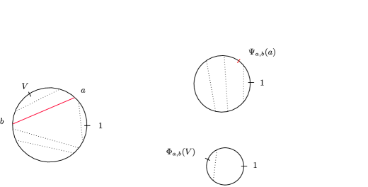
Figure 4: Illustration of the proof in the case $V\in R^{\prime\prime}$.

In order to apply Theorem 3.2 to the fragmentation process of Proposition 3.9, we must first calculate the Malthusian exponent associated to $\nu_{D}$. From the definition of $\nu_{D}$, we have for every $p\geq 0$,

$$\kappa_{\nu_{D}}(p)=1-2\int_{0}^{1}duu^{p+2}-4\int_{1/2}^{1}duu(1-u)\bigl{(}u^{p}+(1-u)^{p}\bigr{)}=\frac{p^{2}+3p-2}{p^{2}+5p+6}.$$

Consequently, the only positive real $\beta^{*}$ such that $\kappa_{\nu_{D}}(\beta^{*})=0$ is

$$\beta^{*}=\frac{\sqrt{17}-3}{2}.$$

We also have $\kappa_{\nu_{D}}(0)=-1/3$.

Let $x\in\mathbb{S}_{1}$. From now on, we will write

$$\mathscr{M}^{(\alpha)}_{t}(x)=\sum_{i=1}^{\infty}\mathrm{m}\bigl{(}R_{i}^{(1,x)}(S_{\alpha}(t))\bigr{)}^{\beta^{*}}$$

for the sum of the ${\beta^{*}}$th powers of masses of the fragments of $S_{\alpha}(t)$ separating $x$ from $1$. This makes sense since both $1$ and $x$ a.s. do not belong to $\operatorname{Feet}(S_{\alpha}(t))$.

By applying Theorem 3.2 to the fragmentation process $\mathcal{X}_{\alpha}(t)$, we get:

Corollary 3.11

Let $V$ be a random variable uniformly distributed over $\mathbb{S}_{1}$ and independent of $(S_{\alpha}(t),t\geq 0,\alpha\geq 0)$. Then: [(iii)]

The process $\mathscr{M}^{(\alpha)}_{t}(V)$ is a uniformly integrable martingale and converges almost surely toward a random variable $\mathscr{M}_{\infty}^{V}$ which does not depend on $\alpha\geq 0$. Moreover $\mathscr{M}_{\infty}^{V}>0$ a.s., and $\mathbb{E}[(\mathscr{M}_{\infty}^{V})^{q}]<\infty$ for every real $q\geq 1$.

For every $\alpha>0$, there exists a constant $K_{\nu_{D}}(\alpha)$ such that

$$t^{-\beta^{*}/\alpha}H_{S_{\alpha}(t)}(1,V)\mathop{\stackrel{{\scriptstyle\mathbb{L}^{2}}}{{\longrightarrow}}}\limits_{t\to\infty}K_{\nu_{D}}(\alpha)\mathscr{M}_{\infty}^{V}.$$

There exists a positive random variable $\mathscr{H}_{0}^{V}$ such that

$$e^{-t/3}H_{S_{0}(t)}(1,V)\mathop{\stackrel{{\scriptstyle a.s.}}{{\longrightarrow}}}\limits_{t\to\infty}\mathscr{H}_{0}^{V}.$$

More generally, for every $p\geq 0$, there exists a positive random variable $\mathscr{H}_{p}^{V}$ such that

$$e^{t\kappa_{\nu_{D}}(p)}\sum_{i=0}^{\infty}\mathrm{m}\bigl{(}R_{i}^{(1,V)}(S_{0}(t))\bigr{)}^{p}\mathop{\stackrel{{\scriptstyle a.s.}}{{\longrightarrow}}}\limits_{t\to\infty}\mathscr{H}_{p}^{V}.$$

Remark 3.12.

The convergence in (ii) can be reinforced in the following way. For every $\delta\in\,]0,1[$,

$$\lim_{t\to\infty}\mathbb{E}\Bigl{[}\sup_{\delta t\leq s\leq t}\bigl{|}s^{-\beta^{*}/\alpha}H_{S_{\alpha}(s)}(1,V)-K_{\nu_{D}}(\alpha)\mathscr{M}_{\infty}^{V}\bigr{|}^{2}\Bigr{]}=0.$$ (6)

To see this, fix $\varepsilon\in\,]0,1[$ and choose a subdivision $\delta=\delta_{0}<\delta_{1}<\cdots<\delta_{k}=1$ of $[\delta,1]$ such that $(\delta_{i+1}/\delta_{i})^{\beta^{*}/\alpha}<1+\varepsilon$ for every $0\leq i\leq k-1$. Since the function $s\mapsto H_{S_{\alpha}}(s)(1,V)$ is nondecreasing, we have

$$\sup_{\delta t\leq s\leq t}\bigl{(}s^{-\beta^{*}/\alpha}H_{S_{\alpha}(s)}(1,V)-K_{\nu_{D}}(\alpha)\mathscr{M}_{\infty}^{V}\bigr{)}$$

$$\qquad\leq\sup_{0\leq i\leq k-1}\bigl{(}(\delta_{i}t)^{-\beta^{*}/\alpha}H_{S_{\alpha}(\delta_{i+1}t)}(1,V)-K_{\nu_{D}}(\alpha)\mathscr{M}_{\infty}^{V}\bigr{)}$$

$$\qquad\leq(1+\varepsilon)\sup_{0\leq i\leq k-1}\bigl{(}(\delta_{i+1}t)^{-\beta^{*}/\alpha}H_{S_{\alpha}(\delta_{i+1}t)}(1,V)-K_{\nu_{D}}(\alpha)\mathscr{M}_{\infty}^{V}\bigr{)}$$

$$\qquad\quad{}+\varepsilon K_{\nu_{D}}(\alpha)\mathscr{M}_{\infty}^{V}.$$

Similar manipulations give

$$\sup_{\delta t\leq s\leq t}\bigl{(}K_{\nu_{D}}(\alpha)\mathscr{M}_{\infty}^{V}-s^{-\beta^{*}/\alpha}H_{S_{\alpha}(s)}(1,V)\bigr{)}$$

$$\qquad\leq\sup_{0\leq i\leq k-1}\bigl{(}K_{\nu_{D}}(\alpha)\mathscr{M}_{\infty}^{V}-(\delta_{i+1}t)^{-\beta^{*}/\alpha}H_{S_{\alpha}(\delta_{i}t)}(1,V)\bigr{)}$$

$$\qquad\leq(1-\varepsilon)\sup_{0\leq i\leq k-1}\bigl{(}K_{\nu_{D}}(\alpha)\mathscr{M}_{\infty}^{V}-(\delta_{i}t)^{-\beta^{*}/\alpha}H_{S_{\alpha}(\delta_{i}t)}(1,V)\bigr{)}$$

$$\qquad\quad{}+\varepsilon K_{\nu_{D}}(\alpha)\mathscr{M}_{\infty}^{V}.$$

It follows that

$$\sup_{\delta t\leq s\leq t}\bigl{|}s^{-\beta^{*}/\alpha}H_{S_{\alpha}(s)}(1,V)-K_{\nu_{D}}(\alpha)\mathscr{M}_{\infty}^{V}\bigr{|}$$

$$\qquad\leq 2\sup_{0\leq i\leq k}\bigl{|}(\delta_{i}t)^{-\beta^{*}/\alpha}H_{S_{\alpha}(\delta_{i}t)}(1,V)-K_{\nu_{D}}(\alpha)\mathscr{M}_{\infty}^{V}\bigr{|}+\varepsilon K_{\nu_{D}}(\alpha)\mathscr{M}_{\infty}^{V}.$$

Using property (ii) in Corollary 3.11, we now get

$$\limsup_{t\to\infty}\mathbb{E}\Bigl{[}\sup_{\delta t\leq s\leq t}\bigl{|}s^{-\beta^{*}/\alpha}H_{S_{\alpha}(s)}(1,V)\,{-}\,K_{\nu_{D}}(\alpha)\mathscr{M}_{\infty}^{V}\bigr{|}^{2}\Bigr{]}\,{\leq}\,2\varepsilon^{2}K_{\nu_{D}}(\alpha)^{2}\mathbb{E}[(\mathscr{M}_{\infty}^{V})^{2}],$$

and (6) follows since $\varepsilon$ was arbitrary.

3.4 Fragments separating $1$ from a deterministic point

We now aim at an analogue of the last corollary when $V$ is replaced by a deterministic point $x$ in $\mathbb{S}_{1}$. We will use the position of the first chord to provide the randomness that we need to reduce the proof to the statement of Corollary 3.11. We start by computing explicitly the distributions of certain quantities that arise when describing the evolution of the process after the creation of the first chord. We use the notation of the beginning of the previous subsection.

We fix $r\in\,]0,1[$ and write $x=e^{2i\pi r}$. Consider first the case when $x\in R^{\prime\prime}$, or equivalently $U_{1}<r<U_{2}$. We then set $Y_{1}=\psi_{U_{1},U_{2}}(U_{1})=\frac{U_{1}}{M}$, which represents the position of the distinguished point, corresponding to the endpoints of the first chord, in the disk obtained from $R^{\prime}$ by contracting the first chord. Similarly, $Y_{2}=\phi_{U_{1},U_{2}}(r)=\frac{r-U_{1}}{1-M}$ gives the position of the distinguished point corresponding to $x$ in the the disk obtained from $R^{\prime\prime}$ by the same contraction.

In the case when $r\in\,]0,U_{1}[\,\cup\,]U_{2},1[$ (or equivalently $x\in R^{\prime}$), we take $Y_{2}=0$ and we let $Y_{1}=\psi_{U_{1},U_{2}}(r)$ be the position of the point corresponding to $x$ in the new disk obtained from $R^{\prime}$ by contracting the first chord.

We first evaluate the density of the pair $(Y_{1},Y_{2})$ on the event $\{x\in R^{\prime\prime}\}=\allowbreak\{U_{1}\,{<}\,r\,{<}\,U_{2}\}$. We have, for any nonnegative measurable function $f$ on $[0,1]^{2}$,

$$\mathbb{E}\bigl{[}f(Y_{1},Y_{2}){\mathbf{1}}_{\{U_{1}<r<U_{2}\}}\bigr{]}$$

$$\qquad=2\int\!\!\int_{[0,1]^{2}}du_{1}\,du_{2}\mathbf{1}_{\{u_{1}<r<u_{2}\}}f\biggl{(}\frac{u_{1}}{1-(u_{2}-u_{1})},\frac{r-u_{1}}{u_{2}-u_{1}}\biggr{)}$$

$$\qquad=2r(1-r)\int_{0}^{1}\!\!\int_{0}^{1}ds_{1}\,ds_{2}$$

$$\qquad\quad{}\times f\biggl{(}\frac{rs_{1}}{rs_{1}+(1-r)(1-s_{2})},\frac{r(1-s_{1})}{r(1-s_{1})+(1-r)s_{2}}\biggr{)}.$$

From the obvious change of variables and after tedious calculations, we get

$$\mathbb{E}\bigl{[}f(Y_{1},Y_{2}){\mathbf{1}}_{\{U_{1}<r<U_{2}\}}\bigr{]}=2\int\!\!\int_{\mathscr{D}_{r}}dr_{1}\,dr_{2}\frac{|r_{1}-r||r_{2}-r|}{|r_{1}-r_{2}|^{3}}f(r_{1},r_{2}),$$ (7)

where $\mathscr{D}_{r}$ is the set $\mathscr{D}_{r}=([r,1]\times[0,r])\cup([0,r]\times[r,1])$. Also note that, on the event $\{U_{1}<r<U_{2}\}$, we have $MY_{1}+(1-M)Y_{2}=r$, and thus $M=\frac{r-Y_{2}}{Y_{1}-Y_{2}}$.

We can similarly compute the distribution of $Y_{1}$ on the event $\{U_{1}\,{<}\,U_{2}\,{<}\,r\}$. For any nonnegative measurable function $f$ on $[0,1]$,

$$\mathbb{E}\bigl{[}f(Y_{1}){\mathbf{1}}_{\{U_{1}<U_{2}<r\}}\bigr{]} = 2\int\!\!\int_{[0,1]^{2}}du_{1}\,du_{2}\mathbf{1}_{\{u_{1}<u_{2}<r\}}f\biggl{(}\frac{r-(u_{2}-u_{1})}{1-(u_{2}-u_{1})}\biggr{)}$$

$$= 2r^{2}\int_{0}^{1}\int_{0}^{1}ds_{1}\,ds_{2}\mathbf{1}_{\{s_{1}<s_{2}\}}f\biggl{(}\frac{r(1-(s_{2}-s_{1}))}{1-r(s_{2}-s_{1})}\biggr{)}$$

$$= 2(1-r)^{2}\int_{0}^{r}dr_{1}\frac{r_{1}}{(1-r_{1})^{3}}f(r_{1}).$$

Also notice that $M=\frac{1-r}{1-Y_{1}}$ on the event $\{U_{1}<U_{2}<r\}$.

A similar calculation, or a symmetry argument, shows that the distribution of $Y_{1}$ on the event $\{r<U_{1}<U_{2}\}$ is given by

$$\mathbb{E}\bigl{[}f(Y_{1}){\mathbf{1}}_{\{r<U_{1}<U_{2}\}}\bigr{]}=2r^{2}\int_{r}^{1}dr_{1}\frac{1-r_{1}}{r_{1}^{3}}f(r_{1}).$$ (9)

Note that $M=\frac{r}{Y_{1}}$ on $\{r<U_{1}<U_{2}\}$.

We can now state and prove the main result of this section.

Theorem 3.13

Let $x\in\mathbb{S}_{1}\setminus\{1\}$. [(iii)]

For every $\alpha\geq 0$, the process $\mathscr{M}_{t}^{(\alpha)}(x)$ converges almost surely toward a random variable $\mathscr{M}_{\infty}(x)$ which does not depend on $\alpha$.

We have $\mathscr{M}_{\infty}(x)>0$ a.s. and $\mathbb{E}[\mathscr{M}_{\infty}(x)^{q}]<\infty$ for every $q\geq 1$.

For every $\alpha>0$, we have

$$t^{-\beta^{*}/\alpha}H_{S_{\alpha}(t)}(1,x)\stackrel{{\scriptstyle(\mathbb{P})}}{{\mathop{\longrightarrow}\limits_{t\to\infty}}}K_{\nu_{D}}(\alpha)\mathscr{M}_{\infty}(x),$$

where the constant $K_{\nu_{D}}(\alpha)$ is the same as in Corollary 3.11.

There exists a positive random variable $\mathscr{H}_{0}(x)$ such that

$$e^{-t/3}H_{S_{0}(t)}(1,x)\mathop{\stackrel{{\scriptstyle a.s.}}{{\longrightarrow}}}\limits_{t\to\infty}\mathscr{H}_{0}(x).$$

More generally, for every $p\geq 0$, there exists a positive random variable $\mathscr{H}_{p}(x)$ such that

$$e^{t\kappa_{\nu_{D}}(p)}\sum_{i=0}^{\infty}\mathrm{m}\bigl{(}R_{i}^{(1,x)}(S_{0}(t))\bigr{)}^{p}\stackrel{{\scriptstyle a.s.}}{{\mathop{\longrightarrow}\limits_{t\to\infty}}}\mathscr{H}_{p}(x).$$

As previously, we write $x=e^{2i\pi r}$, where $r\in\,]0,1[$. To simplify notation, we also set, for every $t\geq 0$, and every $\alpha\geq 0$,

$$\mathcal{X}^{x}_{\alpha}(t)=\bigl{(}\mathrm{m}\bigl{(}R_{1}^{(1,x)}(S_{\alpha}(t))\bigr{)},\mathrm{m}\bigl{(}R_{2}^{(1,x)}(S_{\alpha}(t))\bigr{)},\ldots\bigr{)}.$$

Fix $\alpha\geq 0$. Consider first the case when $x$ belongs to $R^{\prime}$. After time $\tau$, the fragments separating $1$ from $x$ will correspond to fragments separating $1$ from $\Psi_{a,b}(x)$ in the disk obtained from $R^{\prime}$ by contracting the first chord. If $F$ is a nonnegative measurable function on the Skorokhod space ${\mathbb{D}}([0,\infty[,{\mathcal{S}}^{\downarrow})$, Lemma 3.7 gives

$$\quad\mathbb{E}\bigl{[}F\bigl{(}\bigl{(}{\mathcal{X}}^{x}_{\alpha}(\tau+t)\bigr{)}_{t\geq 0}\bigr{)}{\mathbf{1}}_{\{x\in R^{\prime}\}}\bigr{]}=\mathbb{E}\bigl{[}F\bigl{(}\bigl{(}M\widetilde{\mathcal{X}}^{\Psi_{a,b}(x)}_{\alpha}(M^{\alpha}t)\bigr{)}_{t\geq 0}\bigr{)}{\mathbf{1}}_{\{x\in R^{\prime}\}}\bigr{]},$$ (10)

where, for every $y\in\mathbb{S}_{1}\setminus\{1\}$, the process $(\widetilde{\mathcal{X}}^{y}_{\alpha}(t))_{t\geq 0}$ is defined from an independent copy $(\widetilde{S}_{\alpha}(t))_{t\geq 0}$ of $(S_{\alpha}(t))_{t\geq 0}$, in the same way as $({\mathcal{X}}^{y}_{\alpha}(t))_{t\geq 0}$ is defined from $(S_{\alpha}(t))_{t\geq 0}$. Note that $\Psi_{a,b}(x)=\exp(2i\pi Y_{1})$ in the notation introduced before the theorem. From formulas (3.4) and (9) and the relations between $M$ and $Y_{1}$, we get

$$\mathbb{E}\bigl{[}F\bigl{(}\bigl{(}{\mathcal{X}}^{x}_{\alpha}(\tau+t)\bigr{)}_{t\geq 0}\bigr{)}{\mathbf{1}}_{\{x\in R^{\prime}\}}\bigr{]}$$

$$\qquad=2(1-r)^{2}\int_{0}^{r}dr_{1}\frac{r_{1}}{(1-r_{1})^{3}}$$

$$\qquad\quad{}\times\mathbb{E}\biggl{[}F\biggl{(}\biggl{(}\biggl{(}\frac{1-r}{1-r_{1}}\biggr{)}\widetilde{\mathcal{X}}^{\exp(2i\pi r_{1})}_{\alpha}\biggl{(}\biggl{(}\frac{1-r}{1-r_{1}}\biggr{)}^{\alpha}t\biggr{)}\biggr{)}_{t\geq 0}\biggr{)}\biggr{]}$$

$$\qquad\quad{}+2r^{2}\int_{r}^{1}dr_{1}\frac{1-r_{1}}{r_{1}^{3}}\mathbb{E}\biggl{[}F\biggl{(}\biggl{(}\biggl{(}\frac{r}{r_{1}}\biggr{)}\widetilde{\mathcal{X}}^{\exp(2i\pi r_{1})}_{\alpha}\biggl{(}\biggl{(}\frac{r}{r_{1}}\biggr{)}^{\alpha}t\biggr{)}\biggr{)}_{t\geq 0}\biggr{)}\biggr{]}.$$

Let $U$ be uniformly distributed over $[0,1]$ and independent of $(\widetilde{S}_{\alpha}(t))_{t\geq 0}$. By the preceding display, the conditional distribution of $({\mathcal{X}}^{x}_{\alpha}(\tau+t))_{t\geq 0}$ given that $x\in R^{\prime}$ is absolutely continuous (even with a bounded density) with respect to that of the process

$$\biggl{(}{\mathbf{1}}_{\{U<r\}}\frac{1-r}{1-U}\widetilde{\mathcal{X}}^{\exp(2i\pi U)}_{\alpha}\biggl{(}\biggl{(}\frac{1-r}{1-U}\biggr{)}^{\alpha}t\biggr{)}$$

$$\qquad\quad+{\mathbf{1}}_{\{U>r\}}\frac{r}{U}\widetilde{\mathcal{X}}^{\exp(2i\pi U)}_{\alpha}\biggl{(}\biggl{(}\frac{r}{U}\biggr{)}^{\alpha}t\biggr{)}\biggr{)}_{t\geq 0}.$$

Since $V=\exp(2i\pi U)$ is uniformly distributed on $\mathbb{S}_{1}$ and independent of $(\widetilde{S}_{\alpha}(t))_{t\geq 0}$, we can apply Corollary 3.11 to get asymptotics for the process in the last display. It follows that the almost sure convergences in parts (i) and (iv) of the proposition hold on the event $\{x\in R^{\prime}\}$. Moreover the variable $\mathscr{M}_{\infty}(x)$ obtained as the almost sure limit of $\mathscr{M}_{t}^{(\alpha)}(x)$ (only on the event $\{x\in R^{\prime}\}$ for the moment) does not depend on the choice of $\alpha\geq 0$. To see this, note that if we fix two values $\alpha\geq 0$ and $\alpha^{\prime}\geq 0$, the preceding absolute continuity property holds in a similar form for the pair $(({\mathcal{X}}^{x}_{\alpha}(\tau+t))_{t\geq 0},({\mathcal{X}}^{x}_{\alpha^{\prime}}(\tau+t))_{t\geq 0})$. Then it suffices to use the fact that the limiting variable ${\mathscr{M}}_{\infty}^{V}$ in Corollary 3.11(i) does not depend on the choice of $\alpha\geq 0$.

The justification of property (iii) of the theorem (still on the event $\{x\in R^{\prime}\}$) is a bit trickier because we do not have almost sure convergence in Corollary 3.11(ii). We need the reinforced version of Corollary 3.11(ii) provided by Remark 3.12. We observe that, if $U>r$, the quantity $(r/U)^{\alpha}$ is bounded above by $1$ and bounded below by $r^{\alpha}$, so that (6) gives

$$t^{-\beta^{*}/\alpha}H_{\widetilde{S}_{\alpha}((r/U)^{\alpha}t)}(1,\exp(2i\pi U))\stackrel{{\scriptstyle(\mathbb{L}^{2})}}{{\mathop{\longrightarrow}\limits_{t\to\infty}}}\biggl{(}\frac{r}{U}\biggr{)}^{\beta^{*}}K_{\nu_{D}}(\alpha)\tilde{\mathscr{M}}_{\infty}^{V}$$

on the event $\{U>r\}$ (with an obvious notation for $\tilde{\mathscr{M}}_{\infty}^{V}$). A similar observation holds for the asymptotics of $H_{\widetilde{S}_{\alpha}(((1-r)/(1-U))^{\alpha}t)}(1,\exp(2i\pi U))$ on the event $\{U<r\}$. By combining both asymptotics and using the absolute continuity relation mentioned above, we get that the convergence in probability in assertion (iii) of the proposition holds on the event $\{x\in R^{\prime}\}$.

Let us turn to the case where $x$ belongs to $R^{\prime\prime}$. From Lemma 3.7, we have

$$\quad\mathbb{E}\bigl{[}F\bigl{(}\bigl{(}{\mathcal{X}}^{x}_{\alpha}(\tau+t)\bigr{)}_{t\geq 0}\bigr{)}{\mathbf{1}}_{\{x\in R^{\prime\prime}\}}\bigr{]}$$

$$\quad\qquad=\mathbb{E}\bigl{[}F\bigl{(}\bigl{(}M\widetilde{\mathcal{X}}^{\Psi_{a,b}(a)}_{\alpha}(M^{\alpha}t)$$ (11)

$$\quad\qquad\hphantom{=\mathbb{E}\bigl{[}F\bigl{(}(}{}\mbox{\,$\dot{\cup}$\,}(1-M){\bar{\mathcal{X}}}_{\alpha}^{\Phi_{a,b}(x)}\bigl{(}(1-M)^{\alpha}t\bigr{)}\bigr{)}_{t\geq 0}\bigr{)}{\mathbf{1}}_{\{x\in R^{\prime\prime}\}}\bigr{]},$$

where $\widetilde{X}^{y}_{\alpha}$ and $\bar{X}^{y}_{\alpha}$ are defined in terms of two independent copies $\widetilde{S}_{\alpha}$ and $\bar{S}_{\alpha}$ of $S_{\alpha}$ (and the notation $\dot{\cup}$ has the same meaning as in the proof of Proposition 3.9).

Using now formula (7), we obtain

$$\mathbb{E}\bigl{[}F\bigl{(}\bigl{(}{\mathcal{X}}^{x}_{\alpha}(\tau+t)\bigr{)}_{t\geq 0}\bigr{)}{\mathbf{1}}_{\{x\in R^{\prime\prime}\}}\bigr{]}$$

$$\qquad=2\int\!\!\int_{\mathscr{D}_{r}}dr_{1}\,dr_{2}\frac{|r_{1}-r||r_{2}-r|}{|r_{1}-r_{2}|^{3}}$$

$$\qquad\quad{}\times\mathbb{E}\biggl{[}F\biggl{(}\biggl{(}\biggl{(}\frac{r-r_{2}}{r_{1}-r_{2}}\biggr{)}\widetilde{\mathcal{X}}_{\alpha}^{\exp(2i\pi r_{1})}\biggl{(}\biggl{(}\frac{r-r_{2}}{r_{1}-r_{2}}\biggr{)}^{\alpha}t\biggr{)}$$

$$\hphantom{\times\mathbb{E}\biggl{[}F\biggl{(}\biggl{(}}\qquad\quad\mbox{\,$\dot{\cup}$\,}\biggl{(}\frac{r_{1}-r}{r_{1}-r_{2}}\biggr{)}\bar{\mathcal{X}}_{\alpha}^{\exp(2i\pi r_{2})}\biggl{(}\biggl{(}\frac{r_{1}-r}{r_{1}-r_{2}}\biggr{)}^{\alpha}t\biggr{)}\biggr{)}_{t\geq 0}\biggr{)}\biggr{]}.$$

Hence, if $U$ and $U^{\prime}$ are two independent variables uniformly distributed over $[0,1]$ and independent of $(\widetilde{S}_{\alpha},\bar{S}_{\alpha})$, the distribution of $({\mathcal{X}}^{x}_{\alpha}(\tau+t))_{t\geq 0}$ knowing that $x\in R^{\prime\prime}$ is absolutely continuous with respect to the distribution of

$$\biggl{(}\biggl{(}\frac{r-U^{\prime}}{U-U^{\prime}}\biggr{)}\widetilde{\mathcal{X}}_{\alpha}^{\exp(2i\pi U)}\biggl{(}\biggl{(}\frac{r-U^{\prime}}{U-U^{\prime}}\biggr{)}^{\alpha}t\biggr{)}$$

$$\qquad\mbox{\,$\dot{\cup}$\,}\biggl{(}\frac{U-r}{U-U^{\prime}}\biggr{)}\bar{\mathcal{X}}_{\alpha}^{\exp(2i\pi U^{\prime})}\biggl{(}\biggl{(}\frac{U-r}{U-U^{\prime}}\biggr{)}^{\alpha}t\biggr{)}\biggr{)}_{t\geq 0}$$

conditionally on $(U-r)(U^{\prime}-r)<0$. As in the case $x\in R^{\prime}$, we see that the almost sure convergences in assertions (i) and (iv) of the proposition, on the event $\{x\in R^{\prime\prime}\}$, follow from the analogous convergences in Corollary 3.11. By the same argument as in the case $x\in R^{\prime}$, the almost sure limit ${\mathscr{M}}_{\infty}(x)$ in (i) does not depend on the choice of $\alpha\geq 0$.

To get the convergence in probability in assertion (iii), we again use Remark 3.12. The point is that the quantities $((r-U^{\prime})/(U-U^{\prime}))^{\alpha}$ and $((U-r)/(U-U^{\prime}))^{\alpha}$, which are bounded above by $1$ [recall that we condition on $(U-r)(U^{\prime}-r)<0$], are also bounded below by $\delta>0$ except on a set of small probability. As in the case $x\in R^{\prime}$, the desired result follows from (6).

It remains to prove (ii). The property $\mathscr{M}_{\infty}(x)>0$ a.s. is immediate from the analogous property in Corollary 3.11 and our absolute continuity argument. Then, by applying formulas (10) and (3.4) with a suitable choice of the function $F$, we get, for every nonnegative measurable function $f$ on ${\mathbb{R}}_{+}$,

$$\mathbb{E}[f(\mathscr{M}_{\infty}(x))]$$

$$\qquad=\mathbb{E}\bigl{[}f(\mathscr{M}_{\infty}(x)){\mathbf{1}}_{\{x\in R^{\prime}\}}\bigr{]}+\mathbb{E}\bigl{[}f(\mathscr{M}_{\infty}(x)){\mathbf{1}}_{\{x\in R^{\prime\prime}\}}\bigr{]}$$

$$\qquad=\mathbb{E}\bigl{[}f(M^{\beta^{*}}\tilde{\mathscr{M}}_{\infty}(e^{2i\pi Y_{1}})){\mathbf{1}}_{\{x\in R^{\prime}\}}\bigr{]}$$

$$\qquad\quad{}+\mathbb{E}\bigl{[}f\bigl{(}M^{\beta^{*}}\tilde{\mathscr{M}}_{\infty}(e^{2i\pi Y_{1}})+(1-M)^{\beta^{*}}\bar{\mathscr{M}}_{\infty}(e^{2i\pi Y_{2}})\bigr{)}{\mathbf{1}}_{\{x\in R^{\prime\prime}\}}\bigr{]},$$

where $\tilde{\mathscr{M}}_{\infty}$ and $\bar{\mathscr{M}}_{\infty}$ are the obvious analogues of $\mathscr{M}_{\infty}$ when $S_{\alpha}$ is replaced by $\widetilde{S}_{\alpha}$ and $\bar{S}_{\alpha}$, respectively. Set $\mathscr{M}_{\infty}(1)=0$. We have obtained the identity in distribution

$$\mathscr{M}_{\infty}(x)\stackrel{{\scriptstyle(d)}}{{=}}M^{\beta^{*}}\mathscr{M}^{\prime}_{\infty}(e^{2i\pi Y_{1}})+(1-M)^{\beta^{*}}\mathscr{M}^{\prime\prime}_{\infty}(e^{2i\pi Y_{2}}),$$ (12)

where $\mathscr{M}^{\prime}_{\infty}$ and $\mathscr{M}_{\infty}^{\prime\prime}$ are two independent copies of $\mathscr{M}_{\infty}$, and the pair $(\mathscr{M}^{\prime}_{\infty},\allowbreak\mathscr{M}^{\prime\prime}_{\infty})$ is also independent of $(Y_{1},Y_{2})$. However, from the explicit formulas (7), (3.4) and (9), it is easy to verify that both the density of the law of $Y_{1}$ and the density of the law of $Y_{2}$ conditional on $\{Y_{2}\not=0\}$ are bounded above by a constant depending on $x$ [even though the joint density of the pair $(Y_{1},Y_{2})$ conditional on $\{Y_{2}\not=0\}$ is unbounded]. By Corollary 3.11 we know that, if $U$ is uniformly distributed over $[0,1]$ and independent of the figela process, we have $\mathbb{E}[\mathscr{M}_{\infty}(e^{2i\pi U})^{q}]<\infty$ for every $q\geq 1$. The analogous property for $\mathscr{M}_{\infty}(x)$ then follows from (12) and the preceding observations.

Remark 3.14.

By rotational invariance of the model, point $1$ can be replaced by any point of $\mathbb{S}_{1}$ in Theorem 3.13.

4 Estimates for moments and the continuity of the height process

4.1 Estimates for moments

We first state a proposition giving estimates for the moments of the increments of the process $\mathscr{M}_{\infty}(x)$. These estimates will allow us to apply Kolmogorov’s continuity criterion in order to get information on the Hölder continuity properties of this process. Recall that we take $\mathscr{M}_{\infty}(1)=0$ by convention.

Proposition 4.1

For every $\varepsilon>0$ and every integer $p\geq 1$, there exists a constant $M_{\varepsilon,p}\geq 0$ such that, for every $u\in[0,1]$ we have

$$\mathbb{E}[\mathscr{M}_{\infty}(e^{2i\pi u})^{p}]\leq M_{\varepsilon,p}\bigl{(}u(1-u)\bigr{)}^{p\beta^{*}-\varepsilon}.$$

In the special case $p=1$, we have

$$\mathbb{E}[\mathscr{M}_{\infty}(e^{2i\pi u})]=\frac{\Gamma(2+2\beta^{*})}{\Gamma(1+\beta^{*})^{2}}\bigl{(}u(1-u)\bigr{)}^{\beta^{*}}.$$

The proof of the proposition is given in the next two subsections. This proof relies on the identity in distribution (12) derived in the preceding proof. Using this identity and formulas (7), (3.4) and (9), we will obtain integral equations for the moments of $(\mathscr{M}_{\infty}(x),x\in\mathbb{S}_{1})$. We can explicitly solve the integral equation corresponding to the first moment. We then use Gronwall’s lemma to investigate the behavior of higher moments when $x\in\mathbb{S}_{1}$ is close to $1$.

For every integer $p\geq 1$ and every $r\in[0,1]$, we set

$$m_{p}(r)=\mathbb{E}[\mathscr{M}_{\infty}(e^{2i\pi r})^{p}].$$

4.2 The case $p=1$

Let $r\in\,]0,1[$. Thanks to the identity in distribution (12) and to formulas (7), (3.4) and (9), we obtain the integral equation

$$m_{1}(r) = 2(1-r)^{2}\int_{0}^{r}dr_{1}\frac{r_{1}}{(1-r_{1})^{3}}\biggl{(}\frac{1-r}{1-r_{1}}\biggr{)}^{\beta^{*}}m_{1}(r_{1})$$

$${}+2r^{2}\int_{r}^{1}dr_{1}\frac{1-r_{1}}{r_{1}^{3}}\biggl{(}\frac{r}{r_{1}}\biggr{)}^{\beta^{*}}m_{1}(r_{1})$$

$${}+2\int\!\!\int_{\mathscr{D}_{r}}dr_{1}\,dr_{2}\frac{|r_{1}-r||r_{2}-r|}{|r_{1}-r_{2}|^{3}}$$

$$\quad{}\times\biggl{(}\biggl{(}\frac{r-r_{2}}{r_{1}-r_{2}}\biggr{)}^{\beta^{*}}m_{1}(r_{1})+\biggl{(}\frac{r_{1}-r}{r_{1}-r_{2}}\biggr{)}^{\beta^{*}}m_{1}(r_{2})\biggr{)}.$$

We can rewrite the first two terms in the sum of the right-hand side in the form

$$2\!\int_{0}^{r}\!dr_{1}\!\biggl{(}\!\frac{1}{1\,{-}\,r_{1}}\,{-}\,1\!\biggr{)}\!\biggl{(}\!\frac{1\,{-}\,r}{1\,{-}\,r_{1}}\!\biggr{)}^{\beta^{*}+2}m_{1}(r_{1})\,{+}\,2\!\int_{r}^{1}\!dr_{1}\!\biggl{(}\!\frac{1}{r_{1}}\,{-}\,1\!\biggr{)}\biggl{(}\!\frac{r}{r_{1}}\!\biggr{)}^{\beta^{*}+2}m_{1}(r_{1}).$$

As for the third term, we observe that

$$\int_{0}^{r}dr_{1}\int_{r}^{1}dr_{2}\frac{(r-r_{1})(r_{2}-r)}{(r_{2}-r_{1})^{3}}\biggl{(}\frac{r_{2}-r}{r_{2}-r_{1}}\biggr{)}^{\beta^{*}}m_{1}(r_{1})$$

$$\qquad=\int_{0}^{r}dr_{1}m_{1}(r_{1})(r-r_{1})\int_{r}^{1}dr_{2}\biggl{(}\frac{1}{r_{2}-r_{1}}\biggr{)}^{2}\biggl{(}\frac{r_{2}-r}{r_{2}-r_{1}}\biggr{)}^{\beta^{*}+1}$$

$$\qquad=\int_{0}^{r}dr_{1}m_{1}(r_{1})\frac{1}{\beta^{*}+2}\biggl{(}\frac{1-r}{1-r_{1}}\biggr{)}^{\beta^{*}+2},$$

where we made the change of variables $u=\frac{r_{2}-r}{r_{2}-r_{1}}$ to compute the integral in $dr_{2}$. It follows that the third term in the right-hand side of (4.2) is equal to

$$\frac{4}{\beta^{*}+2}\biggl{(}\int_{0}^{r}dr_{1}\biggl{(}\frac{1-r}{1-r_{1}}\biggr{)}^{\beta^{*}+2}m_{1}(r_{1})+\int_{r}^{1}dr_{1}\biggl{(}\frac{r}{r_{1}}\biggr{)}^{\beta^{*}+2}m_{1}(r_{1})\biggr{)}.$$

Summarizing, we obtain that the function $(m_{1}(r),r\in\,]0,1[)$ solves the integral equation

$$m_{1}(r)=\int_{0}^{1}dug_{r}(u)m_{1}(u),$$ (14)

where, for every $r\in\,]0,1[$,

$$g_{r}(u) = \mathbf{1}_{\{0<u<r\}}\biggl{(}\frac{1-r}{1-u}\biggr{)}^{2+\beta^{*}}\biggl{(}\frac{2}{1-u}-\frac{2\beta^{*}}{\beta^{*}+2}\biggr{)}$$

$${}+\mathbf{1}_{\{r\leq u<1\}}\biggl{(}\frac{r}{u}\biggr{)}^{2+\beta^{*}}\biggl{(}\frac{2}{u}-\frac{2\beta^{*}}{\beta^{*}+2}\biggr{)},$$

is a positive function on $]0,1[$. Elementary calculations, using the fact that $(\beta^{*})^{2}+3\beta^{*}-2=0$, show that $\int_{0}^{1}g_{r}(u)\,dr=1$, for every $u\in\,]0,1[$.

Let $N$ be the operator that maps a function $f\in\mathbb{L}^{1}(]0,1[,dr)$ to the function

$$N(f)(r)=\int_{0}^{1}dug_{r}(u)f(u).$$

Then $N$ is a contraction: If $f_{1},f_{2}\in\mathbb{L}^{1}(]0,1[,dr)$, we have

$$\int_{0}^{1}dr|N(f_{1})(r)-N(f_{2})(r)| \leq \int_{0}^{1}dr\int_{0}^{1}dug_{r}(u)|f_{1}(u)-f_{2}(u)|$$

$$= \int_{0}^{1}du|f_{1}(u)-f_{2}(u)|.$$

The first inequality in the last display is strict unless $f_{1}-f_{2}$ has a.e. a constant sign. It follows that there can be at most one nonnegative function $f\in\mathbb{L}^{1}(]0,1[,dr)$ such that $\int_{0}^{1}drf(r)=1$ and $f$ is a fixed point of $N$.

By (14), $m_{1}$ is a fixed point of $N$. Furthermore, if $V$ is uniformly distributed over $\mathbb{S}_{1}$ and independent of $\mathscr{M}_{\infty}$, we know from Corollary 3.11 that $\mathscr{M}_{\infty}(V)$ is the limit of the uniformly integrable martingale $\mathscr{M}^{(\alpha)}_{t}(V)$ (for any choice of $\alpha\geq 0$) and therefore $\mathbb{E}[\mathscr{M}_{\infty}(V)]=1$. Hence,

$$\int_{0}^{1}drm_{1}(r)=\int_{0}^{1}dr\mathbb{E}[\mathscr{M}_{\infty}(e^{2i\pi r})]=\mathbb{E}[\mathscr{M}_{\infty}(V)]=1.$$

We conclude that the function $f=m_{1}$ is the unique nonnegative function in $\mathbb{L}^{1}(]0,1[,dr)$ such that $\int_{0}^{1}drf(r)=1$ and $f$ is a fixed point of $N$. On the other hand, elementary calculus shows that the function $r\mapsto(r(1-r))^{\beta^{*}}$ is also a fixed point of $N$. Indeed, noting that $2\beta^{*}/(\beta^{*}+2)=1-\beta^{*}$ and using two integration by parts, we get

$$\int_{0}^{r}\biggl{(}\frac{1-r}{1-u}\biggr{)}^{2+\beta^{*}}\biggl{(}\frac{2}{1-u}-\frac{2\beta^{*}}{\beta^{*}+2}\biggr{)}\bigl{(}u(1-u)\bigr{)}^{\beta^{*}}\,du=r^{1+\beta^{*}}(1-r)^{\beta^{*}}$$

and similarly,

$$\int_{r}^{1}\biggl{(}\frac{r}{u}\biggr{)}^{2+\beta^{*}}\biggl{(}\frac{2}{u}-\frac{2\beta^{*}}{\beta^{*}+2}\biggr{)}\bigl{(}u(1-u)\bigr{)}^{\beta^{*}}\,du=r^{\beta^{*}}(1-r)^{\beta^{*}+1}.$$

Therefore, the function

$$e_{\beta^{*}}(r):=\frac{\Gamma(2+2\beta^{*})}{\Gamma(1+\beta^{*})^{2}}\bigl{(}r(1-r)\bigr{)}^{\beta^{*}}$$

is also a fixed point of $N$ such that $\int_{0}^{1}dre_{\beta^{*}}(r)=1$. Consequently we have $m_{1}(r)=e_{\beta^{*}}(r)$ a.e. The equality is in fact true for every $r\in\,]0,1[$ since the integral equation (14) implies that $m_{1}$ is continuous on $]0,1[$. This completes the proof of Proposition 4.1 in the case $p=1$.

4.3 The case $p\geq 2$

From the Hölder inequality, and the case $p=1$, we have for every integer $p\geq 1$ and every $r\in\,]0,1[$,

$$m_{p}(r)\geq\biggl{(}\frac{\Gamma(2+2\beta^{*})}{\Gamma(1+\beta^{*})^{2}}\biggr{)}^{p}\bigl{(}r(1-r)\bigr{)}^{p\beta^{*}}.$$ (15)

We prove by induction on $k\geq 1$, that for every $\varepsilon\in\,]0,1/2[$, there exists a constant $M_{\varepsilon,k}>0$ such that for every $r\in\,]0,1[$,

$$m_{k}(r)\leq M_{\varepsilon,k}\bigl{(}r(1-r)\bigr{)}^{k\beta^{*}-\varepsilon}.$$ (16)

We assume that (16) holds for $k=1,2,\ldots,p-1$, and we prove that this bound also holds for $k=p$.

Similarly as in the case $p=1$, we can use the identity in distribution (12) to get the following integral equation for the functions $m_{p}$:

$$m_{p}(r) = \int_{0}^{r}du\biggl{(}\frac{1-r}{1-u}\biggr{)}^{2+p\beta^{*}}\biggl{(}\frac{2}{1-u}-\frac{2p\beta^{*}}{p\beta^{*}+2}\biggr{)}m_{p}(u)$$

$${}+\int_{r}^{1}du\biggl{(}\frac{r}{u}\biggr{)}^{2+p\beta^{*}}\biggl{(}\frac{2}{u}-\frac{2p\beta^{*}}{p\beta^{*}+2}\biggr{)}m_{p}(u)$$

$${}+2\sum_{k=1}^{p-1}\pmatrix{p\cr k}\int\!\!\int_{\mathscr{D}_{r}}dr_{1}\,dr_{2}$$

$$\hphantom{{}+2\sum_{k=1}^{p-1}}{}\times\frac{|r_{1}-r|^{1+(p-k)\beta^{*}}|r_{2}-r|^{1+k\beta^{*}}}{|r_{1}-r_{2}|^{3+p\beta^{*}}}m_{k}(r_{1})m_{p-k}(r_{2}).$$

The derivation of (4.3) from (12) is exactly similar to that of (14), and we leave details to the reader. Note that, in contrast with the case $p=1$, we now get “interaction terms” involving the products $m_{k}(r)m_{p-k}(r)$. We start with some crude estimates.

Lemma 4.2

For every $p\geq 1$, the function $m_{p}$ is bounded over $]0,1[$. Moreover, for every $u,r\in\,]0,1/2[$, we have

$$m_{p}(u)\leq 2^{p-1}\bigl{(}m_{p}(u+r)+m_{p}(r)\bigr{)}.$$ (18)

For every $r,u\in\,]0,1[$, we set

$$g_{p,r}(u) = \mathbf{1}_{\{0<u<r\}}\biggl{(}\frac{1-r}{1-u}\biggr{)}^{2+p\beta^{*}}\biggl{(}\frac{2}{1-u}-\frac{2p\beta^{*}}{p\beta^{*}+2}\biggr{)}$$

$${}+\mathbf{1}_{\{r<u<1\}}\biggl{(}\frac{r}{u}\biggr{)}^{2+\beta^{*}}\biggl{(}\frac{2}{u}-\frac{2p\beta^{*}}{\beta^{*}+2}\biggr{)}.$$

From (4.3), we have

$$m_{p}(r)\geq\int_{0}^{1}dug_{p,r}(u)m_{p}(u).$$

On the other hand, by using (12) and the inequality $(a+b)^{p}\leq 2^{p-1}(a^{p}+b^{p})$ for $a,b\geq 0$, we get

$$m_{p}(r) \leq 2^{p-1}\bigl{(}\mathbb{E}[M^{p\beta^{*}}\mathscr{M}^{\prime}_{\infty}(e^{2i\pi Y_{1}})^{p}]+\mathbb{E}[(1-M)^{p\beta^{*}}\mathscr{M}^{\prime\prime}_{\infty}(e^{2i\pi Y_{2}})^{p}]\bigr{)}$$

$$= 2^{p-1}\int_{0}^{1}dug_{p,r}(u)m_{p}(u),$$

where the last equality again follows from calculations similar to those leading to (14).

From the explicit form of the function $g_{p,r}$, we see that, for every $\delta\in\,]0,1/2[$, there exist positive constants $c_{\delta,p}$ and $C_{\delta,p}$ such that for all $r\in\,]\delta,1-\delta[$,

$$c_{\delta,p}\int_{0}^{1}m_{p}(u)\,du\leq m_{p}(r)\leq C_{\delta,p}\int_{0}^{1}m_{p}(u)\,du.$$ (19)

If $U$ is uniformly distributed over $[0,1]$, Corollary 3.11 shows that$\int_{0}^{1}m_{p}(u)\,du=\mathbb{E}[\mathscr{M}_{\infty}(U)^{p}]<\infty$. We thus get that the function $m_{p}$ is bounded over every compact subset of $]0,1[$.

To get information about the values of the function $m_{p}$ in the neighborhood of $0$ (or of $1$), we use the triangle inequality for figelas. Let $\alpha>0$. For every $r,u\in\,]0,1/2[$ and every $t\geq 0$, Proposition 2.3 gives

$$H_{S_{\alpha}(t)}(1,e^{2i\pi u})\leq H_{S_{\alpha}(t)}\bigl{(}1,e^{2i\pi(u+r)}\bigr{)}+H_{S_{\alpha}(t)}\bigl{(}e^{2i\pi u},e^{2i\pi(u+r)}\bigr{)}.$$

Furthermore, rotational invariance shows that the process $(H_{S_{\alpha}(t)}(e^{2i\pi u},\break e^{2i\pi(u+r)}))_{t\geq 0}$ has the same distribution as the process $(H_{S_{\alpha}(t)}(1,e^{2i\pi r}))_{t\geq 0}$. We thus deduce from Theorem 3.13(iii) that

$$\mathscr{M}_{\infty}(e^{2i\pi u})\leq\mathscr{M}_{\infty}\bigl{(}e^{2i\pi(u+r)}\bigr{)}+\tilde{\mathscr{M}}_{\infty}(e^{2i\pi r}),$$

where $\tilde{\mathscr{M}}_{\infty}(e^{2i\pi r})$ has the same distribution as ${\mathscr{M}}_{\infty}(e^{2i\pi r})$. The bound (18) now follows by using the inequality $(a+b)^{p}\leq 2^{p-1}(a^{p}+b^{p})$ for $a,b\geq 0$.

Since we already know from (19) that the function $m_{p}$ is bounded over compact subsets of $]0,1[$, and since $m_{p}(r)=m_{p}(1-r)$ by an obvious symmetry argument, the bound (18) implies that $m_{p}$ is bounded over $]0,1[$.

We come back to the proof of (16) with $k=p$. We fix $\varepsilon\in\,]0,1/8[$. We start from the integral equation (4.3) and first discuss the interaction terms. Fix $k\in\{1,2,\ldots,p-1\}$ and set, for every $r\in\,]0,1[$,

$$T_{p,k}(r)=\int\!\!\int_{\mathscr{D}_{r}}dr_{1}\,dr_{2}\frac{|r_{1}-r|^{1+(p-k)\beta^{*}}|r_{2}-r|^{1+k\beta^{*}}}{|r_{1}-r_{2}|^{3+p\beta^{*}}}m_{k}(r_{1})m_{p-k}(r_{2}).$$

By the induction hypothesis, there exists a constant $M_{p,k,\varepsilon}$ such that, for $r\in\,]0,1[$,

$$T_{p,k}(r)\leq M_{p,k,\varepsilon}\int\!\!\int_{\mathscr{D}_{r}}dr_{1}\,dr_{2}\frac{|r_{1}-r|^{1+(p-k)\beta^{*}}|r_{2}-r|^{1+k\beta^{*}}}{|r_{1}-r_{2}|^{3+p\beta^{*}}}r_{1}^{k\beta^{*}-\varepsilon}r_{2}^{(p-k)\beta^{*}-\varepsilon}.$$

Consider the integral over $[0,r]\times[r,1]$. From the change of variables $r_{1}=rs_{1}$ and $r_{2}=rs_{2}$, we see that this integral is equal to

$$r^{p\beta^{*}+1-2\varepsilon}\int_{0}^{1}ds_{1}\int_{1}^{1/r}ds_{2}\frac{(1-s_{1})^{1+(p-k)\beta^{*}}(s_{2}-1)^{1+k\beta^{*}}}{(s_{2}-s_{1})^{3+p\beta^{*}}}s_{1}^{k\beta^{*}-\varepsilon}s_{2}^{(p-k)\beta^{*}-\varepsilon}$$

$$\qquad\leq Kr^{p\beta^{*}+1-2\varepsilon},$$

where

$$K=\int_{0}^{1}ds_{1}\int_{1}^{\infty}ds_{2}\frac{(1-s_{1})^{1+(p-k)\beta^{*}}(s_{2}-1)^{1+k\beta^{*}}}{(s_{2}-s_{1})^{3+p\beta^{*}}}s_{2}^{(p-k)\beta^{*}-\varepsilon}<\infty.$$

We get a similar bound for the integral over $[r,1]\times[0,r]$, and, using the fact that $m_{p}(r)=m_{p}(1-r)$, we conclude that the “interaction terms” in the integral equation (4.3) are bounded above by a constant times $(r(1-r))^{p\beta^{*}+1/2}$. By (15) these terms are negligible in comparison with $m_{p}(r)$ when $r\to 0$.

Thus for $r$ sufficiently close to $0$, say $0<r\leq r_{0}\leq 1/4$, we can write

$$m_{p}(r) \leq (1+\varepsilon)\int_{0}^{r}du\biggl{(}\frac{1-r}{1-u}\biggr{)}^{2+p\beta^{*}}\biggl{(}\frac{2}{1-u}-\frac{2p\beta^{*}}{p\beta^{*}+2}\biggr{)}m_{p}(u)$$

$${}+(1+\varepsilon)\int_{r}^{1}du\biggl{(}\frac{r}{u}\biggr{)}^{2+p\beta^{*}}\biggl{(}\frac{2}{u}-\frac{2p\beta^{*}}{p\beta^{*}+2}\biggr{)}m_{p}(u).$$

The first term in the right-hand side is easily bounded by $3\int_{0}^{r}dum_{p}(u)$, and we have, for $0<r\leq r_{0}$,

$$m_{p}(r)\leq 3\!\int_{0}^{r}\!dum_{p}(u)+(1+\varepsilon)\!\int_{r}^{1}\!du\biggl{(}\frac{r}{u}\biggr{)}^{2+p\beta^{*}}\!\biggl{(}\frac{2}{u}-\frac{2p\beta^{*}}{p\beta^{*}+2}\biggr{)}m_{p}(u).$$ (20)

However, by inequality (18), we have for $0<r\leq r_{0}$,

$$\int_{0}^{r}dum_{p}(u)\leq 2^{p-1}\biggl{(}rm_{p}(r)+\int_{r}^{2r}dum_{p}(u)\biggr{)}.$$ (21)

By (4.3), we have also

$$m_{p}(r)\geq\int_{r}^{2r}du\biggl{(}\frac{r}{u}\biggr{)}^{2+p\beta^{*}}\biggl{(}\frac{2}{u}-\frac{2p\beta^{*}}{p\beta^{*}+2}\biggr{)}m_{p}(u),$$

and since $\frac{2}{u}$ tends to infinity as $u\to 0$, this bound shows that $\int_{r}^{2r}dum_{p}(u)$ is negligible in comparison with $m_{p}(r)$ when $r\to 0$. Therefore, from the bound (21) and by choosing $r_{0}$ smaller if necessary, we can assume that, for $0<r\leq r_{0}$,

$$3\int_{0}^{r}dum_{p}(u)\leq\biggl{(}1-\frac{1+\varepsilon}{1+2\varepsilon}\biggr{)}m_{p}(r).$$

By substituting this estimate in (20), we get for $0<r\leq r_{0}$,

$$m_{p}(r)\leq(1+2\varepsilon)\int_{r}^{1}du\biggl{(}\frac{r}{u}\biggr{)}^{2+p\beta^{*}}\biggl{(}\frac{2}{u}-\frac{2p\beta^{*}}{p\beta^{*}+2}\biggr{)}m_{p}(u).$$

Consequently, there exists a positive constant $K=K(r_{0},p,\varepsilon)$ such that for $0<r\leq r_{0}$,

$$\frac{m_{p}(r)}{r^{2+p\beta^{*}}}\leq K+2(1+2\varepsilon)\int_{r}^{r_{0}}\frac{du}{u}\frac{m_{p}(u)}{u^{2+p\beta^{*}}}.$$

A straightforward application of Gronwall’s lemma to the function $r\to r^{-2-p\beta^{*}}\times m_{p}(r)$ gives for $0<r\leq r_{0}$,

$$\frac{m_{p}(r)}{r^{2+p\beta^{*}}}\leq K\biggl{(}\frac{r_{0}}{r}\biggr{)}^{2(1+2\varepsilon)},$$

or equivalently

$$m_{p}(r)\leq Kr_{0}^{2(1+2\varepsilon)}r^{p\beta^{*}-4\varepsilon}.$$

Since $\varepsilon\in\,]0,1/8[$ was arbitrary, and since we have $m_{p}(r)=m_{p}(1-r)$ for $r\in\,]0,1[$, we have obtained the desired bound (16) at order $p$. This completes the proof of Proposition 4.1.

4.4 Proof of Theorem 1.1

The asymptotics in Theorem 1.1 are consequences of the more general results obtained in Corollary 3.6(ii) and in Theorem 3.13(iii), using also Remark 2.7. It remains to verify that the process $(\mathscr{M}_{\infty}(x),x\in\mathbb{S}_{1})$ has a Hölder continuous modification. Let $x$ and $y$ be two distinct points of $\mathbb{S}_{1}\setminus\{0\}$, and let $\alpha>0$. By the triangle inequality in Proposition 2.3, we have for every $t\geq 0$,

$$\bigl{|}H_{S_{\alpha}(t)}(1,x)-H_{S_{\alpha}(t)}(1,y)\bigr{|}\leq H_{S_{\alpha}(t)}(x,y),$$

and $H_{S_{\alpha}(t)}(x,y)$ has the same distribution as $H_{S_{\alpha}(t)}(1,x^{-1}y)$ by rotational invariance. We can let $t\to\infty$ and using Theorem 3.13(iii), we get the following stochastic inequality:

$$|\mathscr{M}_{\infty}(e^{2i\pi{r}})-\mathscr{M}_{\infty}(e^{2i\pi{s}})|\stackrel{{\scriptstyle(d)}}{{\leq}}\mathscr{M}_{\infty}\bigl{(}e^{2i\pi({r}-{s})}\bigr{)}$$ (22)

for every $0\leq s<r<1$.

By Proposition 4.1, we have then for every integer $p\geq 1$ and every $0\leq s<r<1$,

$$\mathbb{E}[|\mathscr{M}_{\infty}(e^{2i\pi{r}})-\mathscr{M}_{\infty}(e^{2i\pi{s}})|^{p}]\leq M_{\varepsilon,p}(r-s)^{p\beta^{*}-\varepsilon}.$$

Kolmogorov’s continuity criterion (see RY99 , Theorem I.2.1) shows that the process $(\mathscr{M}_{\infty}(x),x\in\mathbb{S}_{1})$ has a continuous modification, which is even $(\beta^{*}-\varepsilon)$-Hölder continuous, for every $\varepsilon>0$.

From now on, we only deal with the continuous modification of the process $(\mathscr{M}_{\infty}(x),x\in\mathbb{S}_{1})$. Recall the notation ${\mathcal{T}}_{S}$ for the plane tree associated with a figela $S$, and also recall that $H_{S}$ corresponds to the graph distance on this tree. One may ask about the convergence of the (suitably rescaled) trees ${\mathcal{T}}_{S_{\alpha}(t)}$ in the sense of the Gromov–Hausdorff distance. Recall the notation $T_{g}$ for the $\mathbb{R}$-tree coded by a function $g$ (see Section 2.3).

Set ${g}_{\infty}(r)=\mathscr{M}_{\infty}(e^{2i\pi r})$ for every $r\in[0,1]$. The convergence in distribution

$$\bigl{(}{\mathcal{T}}_{S_{\alpha}(t)},t^{-\beta^{*}/\alpha}H_{S_{\alpha}(t)}\bigr{)}\stackrel{{\scriptstyle(d)}}{{\mathop{\longrightarrow}\limits_{t\to\infty}}}(T_{g_{\infty}},K_{\nu_{D}}(\alpha)\mathrm{d}_{g_{\infty}})$$

holds in the sense of the Gromov–Hausdorff distance.

It would suffice to establish the following convergence in distribution:

$$\bigl{(}t^{-\beta^{*}/\alpha}H_{S_{\alpha}(t)}(1,e^{2i\pi r})\bigr{)}_{r\in[0,1]}\stackrel{{\scriptstyle(d)}}{{\mathop{\longrightarrow}\limits_{t\to\infty}}}(K_{\nu_{D}}(\alpha)\mathscr{M}_{\infty}(e^{2i\pi r}))_{r\in[0,1]}$$

in the Skorokhod sense (the mapping $r\mapsto H_{S_{\alpha}(t)}(1,e^{2i\pi r})$ is not defined when $e^{2i\pi r}$ is a foot of $S_{\alpha}(t)$, but we can choose a suitable convention so that this mapping is defined and càdlàg over $[0,1]$). Proving that this convergence holds would require more information about the process $(H_{S_{\alpha}(t)}(1,x))_{x\in\mathbb{S}_{1},t\geq 0}$.

5 Identifying the limiting lamination

5.1 Preliminaries

The next proposition is the first step toward the proof of Theorem 1.2. We recall the notation introduced at the beginning of Section 3.3: $a=e^{2i\pi U_{1}}$ and $b=e^{2i\pi U_{2}}$ are the feet of the first chord, with $0<U_{1}<U_{2}<1$, and $M=1-(U_{2}-U_{1})$.

Proposition 5.1

Conditionally on the pair $(U_{1},U_{2})$, we have

$$\bigl{(}\mathscr{M}_{\infty}\bigl{(}e^{2i\pi(U_{1}+(U_{2}-U_{1})r)}\bigr{)}-\mathscr{M}_{\infty}(e^{2i\pi U_{1}})\bigr{)}_{r\in[0,1]}\stackrel{{\scriptstyle(d)}}{{=}}\bigl{(}(1-M)^{\beta^{*}}\tilde{\mathscr{M}}_{\infty}(e^{2i\pi r})\bigr{)}_{r\in[0,1]},$$

where $\tilde{\mathscr{M}}_{\infty}$ is copy of $\mathscr{M}_{\infty}$ independent of $M$. Moreover, we have

$$\mathscr{M}_{\infty}(e^{2i\pi U_{1}})>0,\qquad\mbox{a.s.}$$

This is essentially a consequence of Lemma 3.7. Fix $\alpha>0$ and $r\in\,]0,1[$. Using the notation introduced before this lemma, we have on the event $\{U_{1}<r<U_{2}\}$, for every $t\geq 0$,

$$H_{S_{\alpha}(\tau+t)}(1,e^{2i\pi r})=1+H_{S_{\alpha}^{(R^{\prime})}(\tau+t)}(1,e^{2i\pi U_{1}})+H_{S_{\alpha}^{(R^{\prime\prime})}(\tau+t)}(e^{2i\pi U_{1}},e^{2i\pi r}).$$

From Lemma 3.7, we now get on the event $\{U_{1}<r<U_{2}\}$ that conditionally on $(U_{1},U_{2})$,

$$\bigl{(}H_{S_{\alpha}(\tau+t)}(1,e^{2i\pi r})\bigr{)}_{t\geq 0}$$

$$\qquad\stackrel{{\scriptstyle(d)}}{{=}}\bigl{(}1+H_{S^{\prime}_{\alpha}(M^{\alpha}t)}(1,\Psi_{a,b}(a))+H_{S^{\prime\prime}_{\alpha}((1-M)^{\alpha}t)}(1,\Phi_{a,b}(e^{2i\pi r}))\bigr{)}_{t\geq 0}.$$

We multiply each side by $t^{-\beta^{*}/\alpha}$ and pass to the limit $t\to\infty$, using Theorem 3.13(iii), and we get with an obvious notation that, on the event $\{U_{1}<r<U_{2}\}$ and conditionally on $(U_{1},U_{2})$,

$$\mathscr{M}_{\infty}(e^{2i\pi r})\stackrel{{\scriptstyle(d)}}{{=}}M^{\beta^{*}}\mathscr{M}_{\infty}^{\prime}(\Psi_{a,b}(a))+(1-M)^{\beta^{*}}\mathscr{M}_{\infty}^{\prime\prime}\bigl{(}e^{2i\pi\phi_{U_{1},U_{2}}(r)}\bigr{)}.$$

This identity in distribution is immediately extended to a finite number of values of $r$ by the same argument. Noting that $\phi_{U_{1},U_{2}}(U_{1}+(U_{2}-U_{1})r)=r$, we thus get that, conditionally on $(U_{1},U_{2})$,

$$\bigl{(}\mathscr{M}_{\infty}\bigl{(}e^{2i\pi(U_{1}+(U_{2}-U_{1})r)}\bigr{)}\bigr{)}_{r\in[0,1]}$$

$$\qquad\stackrel{{\scriptstyle(d)}}{{=}}\bigl{(}M^{\beta^{*}}\mathscr{M}_{\infty}^{\prime}(\Psi_{a,b}(a))+(1-M)^{\beta^{*}}\mathscr{M}_{\infty}^{\prime\prime}(e^{2i\pi r})\bigr{)}_{r\in[0,1]}.$$

In particular $\mathscr{M}_{\infty}(e^{2i\pi U_{1}})\stackrel{{\scriptstyle(d)}}{{=}}M^{\beta^{*}}\mathscr{M}_{\infty}^{\prime}(\Psi_{a,b}(a))>0$ a.s. by Theorem 3.13(ii), and the identity in distribution of the proposition also follows from the previous display.

Recall the notation $S(\infty)$, $S^{*}(\infty)$ from the end of Section 2.

Lemma 5.2

For every $x\in\mathbb{S}_{1}$, $\mathbb{P}[\exists y\in\mathbb{S}_{1}\setminus\{x\}\dvtx(x,y)\in S^{*}(\infty)]=0$.

Let $\varepsilon>0$. It is enough to prove that, for every $x\in\mathbb{S}_{1}$,

$$\mathbb{P}[\exists y\in\mathbb{S}_{1}\dvtx|y-x|>\varepsilon\mbox{ and }(x,y)\in S^{*}(\infty)]=0.$$

Thanks to rotational invariance, this will follow if we can verify that

$$\mathbb{E}\biggl{[}\int\mathrm{m}(dx){\mathbf{1}}_{\{\exists y\in\mathbb{S}_{1}\dvtx|y-x|>\varepsilon\mbox{ and }(x,y)\in S^{*}(\infty)\}}\biggr{]}=0.$$

Note that if $(x,y)\in S^{*}(\infty)$ the chord $[xy]$ does not cross any of the (other) chords of $S(\infty)$.

We can find an integer $n$ (depending on $\varepsilon$) and $n$ points $z_{1},\ldots,z_{n}$ of $\mathbb{S}_{1}$ such that the following holds. Whenever $x,y\in\mathbb{S}_{1}$ are such that $|y-x|>\varepsilon$, there exists an index $j\in\{1,\ldots,n\}$ such that $z_{j}$ belongs to one of the two open subarcs with endpoints $x$ and $y$, and $-z_{j}$ belongs to the other subarc. If we assume also that $(x,y)\in S^{*}(\infty)$, it follows that $x$ belongs to the boundary of a fragment of $S_{0}(t)$ separating $z_{j}$ from $-z_{j}$, for every $t\geq 0$.

Thanks to these observations, we have for every $t\geq 0$,

$$\int\mathrm{m}(dx){\mathbf{1}}_{\{\exists y\in\mathbb{S}_{1}\dvtx|y-x|>\varepsilon\mathrm{\ and\ }(x,y)\in S^{*}(\infty)\}}\leq\sum_{j=1}^{n}\biggl{(}\sum_{i}\mathrm{m}(R^{z_{j},-z_{j}}_{i}(S_{0}(t)))\biggr{)}$$

with the notation introduced in Definition 3.8. From Theorem 3.13(iv) and the fact that $\kappa_{\nu_{D}}(1)>0$, the right-hand side tends to $0$ almost surely as $t\to\infty$, which completes the proof.

Recall our notation $g_{\infty}(r)=\mathscr{M}_{\infty}(e^{2i\pi r})$ for every $r\in[0,1]$. Notice that $g=g_{\infty}$ satisfies the assumptions of Section 2.3.

Corollary 5.3

Almost surely, for every $r,s\in[0,1]$ such that $\{e^{2i\pi r},\allowbreak e^{2i\pi s}\}\in S(\infty)$, we have $r\stackrel{{\scriptstyle g_{\infty}}}{{\approx}}s$.

If $c,d$ are two distinct points of $\mathbb{S}_{1}\setminus\{1\}$, write $\operatorname{Arc}^{*}(c,d)$ for the open subarc of $\mathbb{S}_{1}$ with endpoints $c$ and $d$ not containing $1$. As an immediate consequence of Proposition 5.1, we have $\mathscr{M}_{\infty}(x)\geq\mathscr{M}_{\infty}(a)=\mathscr{M}_{\infty}(b)>0$, for every $x\in\operatorname{Arc}^{*}(a,b)$. This property is easily extended by induction (using Lemma 3.7 once again) to any chord appearing in the figela process. We have almost surely for every $\{c,d\}\in S(\infty)$,

$$\mathscr{M}_{\infty}(x)\geq\mathscr{M}_{\infty}(c)=\mathscr{M}_{\infty}(d)>0\qquad\mbox{for every }x\in\operatorname{Arc}^{*}(c,d).$$ (23)

We can in fact replace the weak inequality $\mathscr{M}_{\infty}(x)\geq\mathscr{M}_{\infty}(c)$ by a strict one. To see this, we first note that, by Lemma 5.2, $1$ is not an endpoint of a (nondegenerate) chord of $S^{*}(\infty)$. By an easy argument, this implies that almost surely, for every $\varepsilon>0$, there exist $r\in\,]-\varepsilon,0[$ and $s\in\,]0,\varepsilon[$ such that the chord $[e^{2i\pi r}e^{2i\pi s}]$ belongs to $S(\infty)$. It follows that

$$\bigcup_{\{c,d\}\in S(\infty)}\operatorname{Arc}^{*}(c,d)=\mathbb{S}_{1}\setminus\{1\}\qquad\mbox{a.s.}$$

From (23) we now get that $\mathscr{M}_{\infty}(x)>0$, for every $x\in\mathbb{S}_{1}\setminus\{1\}$, a.s.

We can apply this property to the process $\tilde{\mathscr{M}}_{\infty}$ in Proposition 5.1, and we get that $\mathscr{M}_{\infty}(x)>\mathscr{M}_{\infty}(a)=\mathscr{M}_{\infty}(b)$, for every $x\in\operatorname{Arc}^{*}(a,b)$, a.s. Again, this property of the first chord is easily extended by induction to any chord in the figela process, and we obtain that, almost surely for every $\{c,d\}\in S(\infty)$,

$$\mathscr{M}_{\infty}(x)>\mathscr{M}_{\infty}(c)=\mathscr{M}_{\infty}(d)\qquad\mbox{for every }x\in\operatorname{Arc}^{*}(c,d).$$ (24)

The statement of Corollary 5.3 now follows from the definition of $\stackrel{{\scriptstyle g_{\infty}}}{{\approx}}$.

If $(x,y)\in S^{*}(\infty)$ we can write $(x,y)=\lim(x_{n},y_{n})$ where $\{x_{n},y_{n}\}\in S(\infty)$ for every $n$. Write $x=e^{2i\pi r}$, $y=e^{2i\pi s}$ and $x_{n}=e^{2i\pi r_{n}}$, $y_{n}=e^{2i\pi s_{n}}$, where $r,s,\allowbreak r_{n},s_{n}\in[0,1]$. By Corollary 5.3, we have $r_{n}\stackrel{{\scriptstyle g_{\infty}}}{{\approx}}s_{n}$ for every $n$. Since the graph of the relation $\stackrel{{\scriptstyle g_{\infty}}}{{\approx}}$ is closed, it follows that $r\stackrel{{\scriptstyle g_{\infty}}}{{\approx}}s$. We have thus proved that

$$L_{\infty}\subset L_{g_{\infty}}.$$

The reverse inclusion will be proved in the next subsection.

5.2 Maximality of the limiting lamination

The proof of Theorem 1.2 will be completed thanks to the following proposition.

Proposition 5.4

Almost surely, $L_{\infty}$ is a maximal lamination of $\overline{\mathbb{D}}.$

Before proving Proposition 5.4, we need to establish a preliminary lemma. This lemma is concerned with the genealogical tree of fragments appearing in the figela process, which we construct as follows. We consider the fragments created by $S_{0}(t)$ as time increases. The first fragment is $R_{\varnothing}=\overline{\mathbb{D}}$. At the exponential time $\tau$, the first chord splits $\overline{\mathbb{D}}$ into two fragments, which are viewed as the offspring of $\varnothing$. We then order these fragments in a random way: with probability $1/2$, we call $R_{0}$ the fragment with the largest mass and $R_{1}$ the other one, and with probability $1/2$ we do the contrary. We then iterate this device. Then each fragment that appears in the figela process is labeled by an element of the infinite binary tree

$$\mathbb{T}=\bigcup_{n\geq 0}\{0,1\}^{n}.$$

For every integer $n$, we also set

$$\mathbb{T}_{n}:=\bigcup_{k=0}^{n}\{0,1\}^{k}.$$

At every time $t$, we have a (finite) binary tree corresponding to the genealogy of the fragments present at time $t$. See Figure 5.

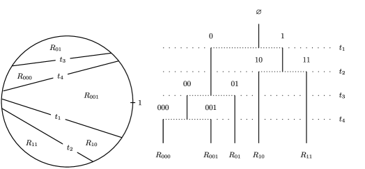
Figure 5: Chords are represented on the left-hand side with their respective creation times. On the right-hand side the genealogical tree of the fragments $R_{000},\ldots,R_{11}$ present at time $t_{4}$.

If $R$ is a fragment, we call end of $R$ any connected component of $R\cap\mathbb{S}_{1}$. We denote the number of ends of a fragment $R$ by $\mathrm{e}(R).$ For reasons that will be explained later, the full disk $\overline{\mathbb{D}}$ is viewed as a fragment with $0$ end.

Lemma 5.5

In the (infinite) genealogical tree of fragments, almost surely, there is no ray along which all fragments have eventually strictly more than 3 ends.

Let $n\geq 0$ and $u\in\{0,1\}^{n}$, and consider the fragment $R_{u}$. Let $y_{u}$ be one endpoint (chosen at random) of the first chord that will fall inside $R_{u}$. Note that, conditionally on $R_{u}$, $y_{u}$ is uniformly distributed over $R_{u}\cap\mathbb{S}_{1}$. Let $\varphi_{u}\dvtx[0,\mathrm{m}(R_{u})[\longrightarrow\overline{R_{u}\cap\mathbb{S}_{1}}$ be defined by requiring that the measure of the intersection of $R_{u}\cap\mathbb{S}_{1}$ with the arc (in counterclockwise order) between $y_{u}$ and $\varphi_{u}(t)$ is equal to $t$, for every $t\in[0,\mathrm{m}(R_{u})[$. This definition is unambiguous if we also impose that $\varphi_{u}$ is right-continuous. Then $\varphi_{u}$ has exactly $\mathrm{e}(R_{u})$ discontinuity times corresponding to the chords that lie in the boundary of $R_{u}$ (indeed the left and right limits of $\varphi_{u}$ at a discontinuity time are the endpoints of a chord adjacent to $R_{u}$). We claim that, conditionally given $(\mathrm{m}(R_{u}),\mathrm{e}(R_{u}))$, the set of discontinuity times of $\varphi_{u}$ is distributed as the collection of $\mathrm{e}(R_{u})$ independent points chosen uniformly over $[0,\mathrm{m}(R_{u})[$.

This claim can be checked by induction on $n$. For $n=0$ there is nothing to prove. Assume that the claim holds up to order $n$. Recalling that $y_{u}$ is one endpoint of the first chord that will fall in $R_{u}$, the other endpoint $z_{u}$ will be chosen uniformly over $R_{u}\cap\mathbb{S}_{1}$, so that $\varphi_{u}^{-1}(z_{u})$ will be uniform over $[0,\mathrm{m}(R_{u})[$. We have then $\mathrm{e}(R_{u0})=K+1$ and $\mathrm{e}(R_{u1})=\mathrm{e}(R_{u})+1-K$ (or the contrary with probability $1/2$), where $K$ is the number of discontinuity times of $\varphi_{u}$ in $[0,\varphi_{u}^{-1}(z_{u})]$. Using our induction hypothesis, we see that conditionally on $K$ and on $\varphi_{u}^{-1}(z_{u})$ the latter discontinuity times are independent and uniformly distributed over $[0,\varphi_{u}^{-1}(z_{u})]$, and that a similar property holds for the discontinuity times that belong to $[\varphi_{u}^{-1}(Z_{u}),\mathrm{m}(R_{u})]$. It follows that the desired property will still hold at order $n+1$.

The preceding arguments also show that, conditionally on $R_{u}$, $\mathrm{e}(R_{u0})$ is distributed as $K+1$, where $K$ is obtained by throwing $\mathrm{e}(R_{u})+1$ uniform random variables in $[0,\mathrm{m}(R_{u})]$ and counting how many among the $\mathrm{e}(R_{u})$ first ones are smaller than the last one. By an obvious symmetry argument, we have, for any integers $p\geq 0$, $k\in\{0,\ldots,p\}$ and any $a\in\,]0,1]$,

$$\mathbb{P}[\mathrm{e}(R_{u0})=k+1|\mathrm{e}(R_{u})=p,\mathrm{m}(R_{u})=a]=\frac{1}{p+1}.$$

Notice that the preceding conditional probability does not depend on $a$, which could have been seen from a scaling argument.

Modulo some technical details that are left to the reader, we get that the distribution of the tree-indexed process $(\mathrm{e}(R_{u}),u\in\mathbb{T})$ can be described as follows. We start with $\mathrm{e}(\varnothing)=0$, and we then proceed by induction on $n$ to define $\mathrm{e}(R_{u})$ for every $u\in\{0,1\}^{n}$. To this end, given the values of $\mathrm{e}(R_{u})$ for $u\in\mathbb{T}_{n}$, we choose independently for every $v\in\{0,1\}^{n}$ a random variable $k_{v}$ uniform over $\{0,\ldots,\mathrm{e}(R_{v})\}$, and we set $\mathrm{e}(R_{v0})=k_{v}+1$, $\mathrm{e}(R_{v1})=\mathrm{e}(R_{v})-k_{v}+1$.

Consider a tree-indexed process $(\mathrm{f}_{u},u\in\mathbb{T})$ that evolves according to the preceding rules but starts with $\mathrm{f}_{\varnothing}=4$ [instead of $\mathrm{e}(R_{\varnothing})=0$]. In order to get the statement of the lemma, it is enough to prove that almost surely, there is no infinite ray starting from the root along which all the values of $\mathrm{f}_{u}$ are strictly larger than $3$. Consider a fixed infinite ray in the tree, say $\varnothing,0,00,\allowbreak 000,\ldots$ and let $X_{0}=\mathrm{f}_{\varnothing}$, $X_{1}=\mathrm{f}_{0}$, $X_{2}=\mathrm{f}_{00},\ldots$ be the values of our process along the ray. Note that $(X_{n})_{n\geq 0}$ is a Markov chain with values in $\mathbb{N}$, with transition kernel given by

$$q_{k\ell}=\frac{1}{k+1}\mathbf{1}_{\{1\leq l\leq k+1\}}$$

for every $k,\ell\geq 1$. Write $(\mathcal{F}_{n})_{n\geq 0}$ for the filtration generated by the process $(X_{n})_{n\geq 0}$. We have

$$\mathbb{E}[X_{n+1}|\mathcal{F}_{n}]=\frac{1}{X_{n}+1}\bigl{(}1+2+\cdots+(X_{n}+1)\bigr{)}=\frac{X_{n}}{2}+1.$$

Hence $M_{n}=2^{n}(X_{n}-2)$ is a martingale starting from $2$. For $i\geq 1$ we let $T_{i}$ be the stopping time $T_{i}=\inf\{n\geq 0\dvtx X_{n}=i\},$ and $T=T_{1}\wedge T_{2}\wedge T_{3}$.

Note that $\mathbb{P}[X_{k}\geq 4,\mbox{ for every }0\leq k\leq n]=\mathbb{P}[T>n]$, and that the preceding discussion applies to the values of $f_{u}$ along any infinite ray starting from the root.

By the stopping theorem applied to the martingale $(M_{n})_{n\geq 0}$, we obtain for every $n\geq 0$,

$$2 = \mathbb{E}[M_{n\wedge T}]$$

$$= \mathbb{E}\bigl{[}-2^{T_{1}}\mathbf{1}_{\{T_{1}=T\leq n\}}\bigr{]}+0+\mathbb{E}\bigl{[}2^{T_{3}}\mathbf{1}_{\{T_{3}=T\leq n\}}\bigr{]}+\mathbb{E}\bigl{[}2^{n}(X_{n}-2)\mathbf{1}_{\{T>n\}}\bigr{]}.$$

From the transition kernel of the Markov chain $(X_{n})_{n\geq 0}$ it is easy to check that for every $k\geq 1$, $\mathbb{P}[T_{1}=T=k]=\mathbb{P}[T_{2}=T=k]=\mathbb{P}[T_{3}=T=k].$ Hence, the equality in the last display becomes

$$2=\mathbb{E}\bigl{[}2^{n}(X_{n}-2)\mathbf{1}_{\{T>n\}}\bigr{]},$$

or equivalently

$$2=2^{n}\mathbb{P}[T>n]\mathbb{E}[X_{n}-2\mid T>n].$$

Since obviously $\mathbb{E}[X_{n}-2\mid T>n]\geq 2$, we get $2^{n}\mathbb{P}[T>n]\leq 1$.

For every $u=(u_{1},\ldots,u_{n})\in\{0,1\}^{n}$, and every $j\in\{0,1,\ldots,n\}$, set $[u]_{j}=(u_{1},\ldots,u_{j})$, and if $j\geq 1$, also set $[u]_{j}^{*}=(u_{1},\ldots,u_{j-1},1-u_{j})$. Let

$$G_{n}=\bigl{\{}u\in\{0,1\}^{n}\dvtx\mathrm{f}_{[u]_{j}}\geq 4,\forall j\in\{0,1,\ldots,n\}\bigr{\}}.$$

Clearly

$$\mathbb{E}[\#G_{n}]=2^{n}\mathbb{P}[T>n]\leq 1.$$ (25)

In order to get the statement of the lemma, it is enough to verify that $\mathbb{P}[\#G_{n}\geq 1]\longrightarrow 0$ as $n\to\infty$. Note that the sequence $\mathbb{P}[\#G_{n}\geq 1]$ is monotone nonincreasing. We argue by contradiction and assume that there exists $\eta>0$ such that $\mathbb{P}[\#G_{n}\geq 1]\geq\eta$ for every $n\geq 1$. By a simple coupling argument, the same lower bound will remain valid if we start the tree-indexed process with $\mathrm{f}_{\varnothing}=m$, for any $m\geq 4$, instead of $\mathrm{f}_{\varnothing}=4$.

Fix $\varepsilon\in\,]0,\eta[$, and choose an integer $\ell\geq 1$ such that $1/\ell\leq\varepsilon/2$. Choose another integer $k\geq 1$ such that, if $B_{k,\eta}$ denotes a binomial ${\mathcal{B}}(k,\eta)$ random variable, we have $\mathbb{P}[B_{k,\eta}\leq\ell]\leq\varepsilon/2$. Finally set

$$G^{\prime}_{n} = \bigl{\{}u\in G_{n}\dvtx\#\bigl{\{}j\in\{0,1,\ldots,n-1\}\dvtx\mathrm{f}_{[u]_{j+1}}\leq\mathrm{f}_{[u]_{j}}-2\bigr{\}}\leq k\bigr{\}},$$

$$G^{\prime\prime}_{n} = G_{n}\setminus G^{\prime}_{n}.$$

We first evaluate $\mathbb{P}[G^{\prime\prime}_{n}\not=\varnothing]$. We have

$$\mathbb{P}[G^{\prime\prime}_{n}\not=\varnothing]\leq\mathbb{P}[G^{\prime\prime}_{n}\not=\varnothing,\#G_{n}\leq\ell]+\mathbb{P}[\#G_{n}>\ell].$$

By (25) and our choice of $\ell$, we have $\mathbb{P}[\#G_{n}>\ell]\leq\ell^{-1}\mathbb{E}[\#G_{n}]\leq\varepsilon/2$. On the other hand,

$$\mathbb{P}[G^{\prime\prime}_{n}\not=\varnothing,\#G_{n}\leq\ell] \leq \mathbb{E}\bigl{[}\#G^{\prime\prime}_{n}{\mathbf{1}}_{\{\#G_{n}\leq\ell\}}\bigr{]}$$

$$= \sum_{u\in\{0,1\}^{n}}\mathbb{P}[u\in G^{\prime\prime}_{n},\#G_{n}\leq\ell]$$

$$= \sum_{u\in\{0,1\}^{n}}\mathbb{P}[u\in G^{\prime\prime}_{n}]\mathbb{P}[\#G_{n}\leq\ell|u\in G^{\prime\prime}_{n}].$$

Fix $u\in\{0,1\}^{n}$. We argue conditionally on the values of $\mathrm{f}_{[u]_{j}}$ for $0\leq j\leq n$, and note that the values of $\mathrm{f}_{[u]_{j+1}^{*}}$ for $0\leq j\leq n-1$ are then also determined by the condition $\mathrm{f}_{[u]_{j+1}}+\mathrm{f}_{[u]_{j+1}^{*}}=\mathrm{f}_{[u]_{j}}+2$. Moreover, on the event $\{u\in G^{\prime\prime}_{n}\}$, there are at least $k$ values of $j\in\{0,1,\ldots,n-1\}$ such that $\mathrm{f}_{[u]_{j+1}}\leq\mathrm{f}_{[u]_{j}}-2$. For these values of $j$, we must have $\mathrm{f}_{[u]_{j+1}^{*}}\geq 4$. Furthermore, for each such value of $j$, there is (conditional) probability at least $\eta$ that one of the descendants of $[u]^{*}_{j+1}$ at generation $n$, say $v$, is such that $\mathrm{f}_{[v]_{i}}\geq 4$ for every $i\in\{j+1,\ldots,n\}$, and consequently $v\in G_{n}$. Summarizing, we see that conditionally on the event $\{u\in G^{\prime\prime}_{n}\}$, $\#G_{n}$ is bounded below in distribution by a binomial ${\mathcal{B}}(k,\eta)$ random variable. Hence, using our choice of $k$,

$$\mathbb{P}[\#G_{n}\leq\ell|u\in G^{\prime\prime}_{n}]\leq\mathbb{P}[B_{k,\eta}\leq\ell]\leq\frac{\varepsilon}{2}.\vspace*{-1pt}$$

We thus get

$$\mathbb{P}[G^{\prime\prime}_{n}\not=\varnothing,\#G_{n}\leq\ell]\leq\frac{\varepsilon}{2}\sum_{u\in\{0,1\}^{n}}\mathbb{P}[u\in G^{\prime\prime}_{n}]=\frac{\varepsilon}{2}\mathbb{E}[\#G^{\prime\prime}_{n}]\leq\frac{\varepsilon}{2},\vspace*{-1pt}$$

by (25). It follows that

$$\limsup_{n\to\infty}\mathbb{P}[G^{\prime\prime}_{n}\not=\varnothing]\leq\varepsilon.\vspace*{-1pt}$$

We will now verify that $\mathbb{P}[G^{\prime}_{n}\not=\varnothing]$ tends to $0$ as $n\to\infty$. Since $\varepsilon<\eta$, this will give a contradiction with our assumption $\mathbb{P}[\#G_{n}\geq 1]\geq\eta$ for every $n\geq 1$, thus completing the proof. We in fact show that $\mathbb{E}[\#G^{\prime}_{n}]$ tends to $0$ as $n\to\infty$. To this end, we first write, for $n\geq k$,

$$\mathbb{E}[\#G^{\prime}_{n}] = 2^{n}\mathbb{P}[T>n,\#\bigl{\{}j\in\{0,\ldots,n-1\}\dvtx X_{j+1}\leq X_{j}-2\bigr{\}}\leq k]$$

$$\leq 2^{n}n^{k}\sup_{A\subset\{0,1,\ldots,n-1\},\#A=k}\mathbb{P}[X_{j+1}\geq(X_{j}-1)\vee 4,$$

$$\hphantom{\;2^{n}n^{k}\sup_{A\subset\{0,1,\ldots,n-1\},\#A=k}\mathbb{P}}\forall j\in\{0,1,\ldots,n-1\}\setminus A].\vspace*{-1pt}$$

We thus need to bound the quantity

$$\mathbb{P}[X_{j+1}\geq(X_{j}-1)\vee 4,\forall j\in\{0,1,\ldots,n-1\}\setminus A],\vspace*{-1pt}$$

for every choice of $A\subset\{0,1,\ldots,n-1\}$ such that $\#A=k$. For every subset $A$ of $\{0,1,\ldots,n-1\}$, we set

$$N^{A}_{n}=\#\bigl{\{}j\in\{0,1,\ldots,n-1\}\setminus A\dvtx X_{j}=5\bigr{\}}.\vspace*{-1pt}$$

With a slight abuse of notation, write $\mathbb{P}_{i}$ for a probability measure under which the Markov chain $X$ starts from $i$. We prove by induction on $n$ that for every choice of $A\subset\{0,1,\ldots,n-1\}$ and $m\in\{0,1,\ldots,n-\#A\}$, we have for every $i\geq 1$,

$${\mathbb{P}}_{i}[X_{j+1}\geq(X_{j}-1)\vee 4,\forall j\in\{0,1,\ldots,n-1\}\setminus A;N^{A}_{n}=m]$$

(27)

$$\qquad\leq\biggl{(}\frac{1}{2}\biggr{)}^{m}\biggl{(}\frac{3}{7}\biggr{)}^{n-m-\#A}.$$

If $n=0$ (then necessarily $m=0$ and $A=\varnothing$) there is nothing to prove. Assume that the desired bound holds at order $n-1$. In order to prove that it holds at order $n$, we apply the Markov property at time $1$. We need to distinguish three cases.

If $0\in A$, then the left-hand side of (5.2) is equal to

$$\sum_{i^{\prime}}q_{ii^{\prime}}\mathbb{P}_{i^{\prime}}[X_{j+1}\geq(X_{j}-1)\vee 4,\forall j\in\{0,1,\ldots,n-2\}\setminus A^{\prime};N^{A^{\prime}}_{n-1}=m],$$

where $A^{\prime}=\{j-1\dvtx j\in A,j>0\}$. Since $\#A^{\prime}=\#A-1$ in that case, an application of the induction hypothesis gives the result.

If $0\notin A$ and $i\not=5$, then the left-hand side of (5.2) is equal to

$$\sum_{i^{\prime}\geq(i-1)\vee 4}q_{ii^{\prime}}\mathbb{P}_{i^{\prime}}[X_{j+1}\geq(X_{j}-1)\vee 4,\forall j\in\{0,1,\ldots,n-2\}\setminus A^{\prime};N^{A^{\prime}}_{n-1}=m]$$

$$\qquad\leq\sum_{i^{\prime}\geq(i-1)\vee 4}q_{ii^{\prime}}\biggl{(}\frac{1}{2}\biggr{)}^{m}\biggl{(}\frac{3}{7}\biggr{)}^{n-1-m-\#A^{\prime}},$$

and we just have to observe that

$$\sum_{i^{\prime}\geq(i-1)\vee 4}q_{ii^{\prime}}\leq\frac{3}{7}$$

when $i\not=5$.

Finally, if $0\notin A$ and $i=5$, the left-hand side of (5.2) is equal to

$$\sum_{i^{\prime}\geq 4}q_{5i^{\prime}}\mathbb{P}_{i^{\prime}}[X_{j+1}\geq(X_{j}-1)\vee 4,\forall j\in\{0,1,\ldots,n-2\}\setminus A^{\prime};N^{A^{\prime}}_{n-1}=m-1]$$

$$\qquad\leq\biggl{(}\sum_{i^{\prime}\geq 4}q_{5i^{\prime}}\biggr{)}\biggl{(}\frac{1}{2}\biggr{)}^{m-1}\biggl{(}\frac{3}{7}\biggr{)}^{(n-1)-(m-1)-\#A^{\prime}}$$

$$\qquad=\biggl{(}\frac{1}{2}\biggr{)}^{m}\biggl{(}\frac{3}{7}\biggr{)}^{n-m-\#A},$$

using the fact that $\sum_{i^{\prime}\geq 4}q_{5i^{\prime}}=1/2$. This completes the proof of (5.2).

Fix $\delta\in\,]0,1[$. By summing over possible values of $m$, we get for $n$ large, for all choices of $A\subset\{0,1,\ldots,n-1\}$ such that $\#A=k$

$$\mathbb{P}[X_{j+1}\geq(X_{j}-1)\vee 4,\forall j\in\{0,1,\ldots,n-1\}\setminus A]$$

$$\qquad\leq\sum_{m=0}^{n-\lfloor\delta n\rfloor}\biggl{(}\frac{1}{2}\biggr{)}^{m}\biggl{(}\frac{3}{7}\biggr{)}^{n-m-k}+\mathbb{P}[N^{A}_{n}>n-\lfloor\delta n\rfloor]$$

$$\qquad\leq n\biggl{(}\frac{1}{2}\biggr{)}^{n-\lfloor\delta n\rfloor}\biggl{(}\frac{3}{7}\biggr{)}^{\lfloor\delta n\rfloor-k}+\mathbb{P}[N^{A}_{n}>n-\lfloor\delta n\rfloor].$$

Note that $N^{A}_{n}\leq N^{\varnothing}_{n}$. Crude estimates, using the fact that $\sup_{i\geq 1}q_{i5}=1/5$, show that we can fix $\delta$ such that

$$2^{n}n^{k+1}\mathbb{P}[N^{\varnothing}_{n}>n-\lfloor\delta n\rfloor]\mathop{\longrightarrow}\limits_{n\to\infty}0.$$

It then follows that the right-hand side of (5.2) tends to $0$ as $n\to\infty$, which completes the proof.

Remark 5.6.

For every integer $k\geq 1$, let $(\mathrm{f}^{(k)}_{u},u\in\mathbb{T})$ be a tree-indexed process that evolves according to the same rules as $(\mathrm{e}(R_{u}),u\in\mathbb{T})$ but starts with $\mathrm{f}^{(k)}_{\varnothing}=k$. Let $p_{k}$ be the probability that there exists no infinite ray starting from $\varnothing$ along which all labels $\mathrm{f}^{(k)}_{u}$ are strictly greater than $3$. By conditioning on the values of $\mathrm{f}^{(k)}_{0}$ and $\mathrm{f}^{(k)}_{1}$, we see that $(p_{k})_{k\geq 1}$ satisfies the properties

$$\quad\cases{\displaystyle p_{1}=p_{2}=p_{3}=1,\vspace*{2pt}\cr\displaystyle p_{k}=\frac{1}{k+1}(p_{1}p_{k+1}+p_{2}p_{k}+\cdots+p_{k}p_{2}+p_{k+1}p_{1}),&\quad if $k\geq 4$.}$$ (28)

It follows that the values of $p_{k}$ for $k\geq 5$ are determined recursively from the value of $p_{4}$. Numerical simulations suggest that there exists no sequence $(p_{k})_{k\geq 1}$ satisfying (28) such that $p_{4}<1$ and $0\leq p_{k}\leq 1$ for every $k\geq 1$. A rigorous verification of this fact would provide an alternative more analytic proof of Lemma 5.5.

Proof of Proposition 5.4 First note that it is easy to verify that $L_{\infty}\cap\mathbb{S}_{1}$ is dense in $\mathbb{S}_{1}$, and thus $\mathbb{S}_{1}\subset L_{\infty}$ since $L_{\infty}$ is closed. We argue by contradiction and suppose that $L_{\infty}$ is not a maximal lamination. Then there exists a (nondegenerate) chord $[xy]$ which is not contained in $L_{\infty}$ and is such that $L_{\infty}\cup[xy]$ is still a lamination, which implies that $]xy[$ does not intersect any chord of $S(\infty)$. There is a unique infinite ray $\varnothing,\epsilon_{1},\epsilon_{1}\epsilon_{2},\ldots$ in $\mathbb{T}$ such that $]xy[\subset R_{\epsilon_{1}\cdots\epsilon_{n}}$ for every integer $n\geq 0$. We claim that, for all sufficiently large $n$, $R_{\epsilon_{1}\cdots\epsilon_{n}}$ has at least $4$ ends. To see this, denote by $I^{x}_{n}$ the end of $R_{\epsilon_{1}\cdots\epsilon_{n}}$ whose closure $\overline{I^{x}_{n}}$ contains $x$, and define $I^{y}_{n}$ similarly. Note that the maximal length of an end of a fragment at the $n$th generation tends to $0$ a.s., and that this applies in particular to $I^{x}_{n}$ and $I^{y}_{n}$. It follows that, almost surely for all $n$ sufficiently large, there is no chord of $S(\infty)$ between a point of $\overline{I^{x}_{n}}$ and a point of $\overline{I^{y}_{n}}$ (otherwise, the pair $(x,y)$ would be in $S^{*}(\infty)$ and the chord $[xy]$ would be contained in $L_{\infty}$). Hence, for all sufficiently large $n$, the boundary of $R_{\epsilon_{1}\cdots\epsilon_{n}}$ contains at least $4$ different chords, and therefore at least $4$ ends. This contradicts Lemma 5.5, and this contradiction completes the proof.

Proof of Theorem 1.2 Since $L_{\infty}$ is a maximal lamination and $L_{\infty}\subset L_{g_{\infty}}$, we must have $L_{\infty}=L_{g_{\infty}}$ and in particular $L_{g_{\infty}}$ is a maximal lamination. Thus, the function $g_{\infty}$ must satisfy the necessary and sufficient condition for maximality given in Proposition 2.5. Under this condition, however, the relations $\stackrel{{\scriptstyle g_{\infty}}}{{\approx}}$ and $\stackrel{{\scriptstyle g_{\infty}}}{{\sim}}$ coincide. Recalling that ${\mathscr{M}}_{\infty}(x)>0={\mathscr{M}}_{\infty}(1)$ for every $x\in\mathbb{S}_{1}\setminus\{1\}$, we see that property (1) written with $x=e^{2i\pi r}$ and $y=e^{2i\pi s}$ is equivalent to saying that $r\stackrel{{\scriptstyle g_{\infty}}}{{\sim}}s$. Theorem 1.2 then follows from the fact that $L_{\infty}=L_{g_{\infty}}$.

Remark 5.7.

It is not hard to see that $L_{\infty}$ has zero Lebesgue measure a.s. (this follows from the upper bound on the Hausdorff dimension proved in the next section). By a simple argument, it follows that a chord $[xy]$ is contained in $L_{\infty}$ if and only if $x\stackrel{{\scriptstyle g_{\infty}}}{{\approx}}y$, and this condition is also equivalent to $(x,y)\in S^{*}(\infty)$.

6 The Hausdorff dimension of $L_{\infty}$

In this section, we prove Theorem 1.3. We let ${\mathcal{I}}$ be the countable set of all pairs $(I,J)$ where $I$ and $J$ are two disjoint closed subarcs of $\mathbb{S}_{1}$ with nonempty interior and endpoints of the form $\exp(2i\pi r)$ with rational $r$. For each $(I,J)\in{\mathcal{I}}$, we set

$$L_{(I,J)}=\bigcup_{(y,z)\in S^{*}(\infty)\cap(I\times J)}[yz]\subset L_{\infty}.$$

Clearly,

$$\operatorname{dim}L_{\infty}=\sup_{(I,J)\in{\mathcal{I}}}\operatorname{dim}\bigl{(}L_{(I,J)}\bigr{)}.$$ (29)

Upper bound

We prove that, for every $(I,J)\in{\mathcal{I}}$,

$$\operatorname{dim}\bigl{(}L_{(I,J)}\bigr{)}\leq\frac{\sqrt{17}-1}{2}=\beta^{*}+1\qquad\mbox{a.s.}$$

By rotational invariance, we may assume without loss of generality that $1\notin I\cup J$. We pick a point $x\in\mathbb{S}_{1}\setminus(I\cup J)$ such that $1$ and $x$ belong to different components of $\mathbb{S}_{1}\setminus(I\cup J)$. We also fix $\gamma>\beta^{*}+1$ and set $\beta=\gamma-1>\beta^{*}$.

We consider the figela process $(S_{0}(t),t\geq 0)$ with autosimilarity parameter $\alpha=0$. We fix $t>0$ for the moment and denote the maximal number of ends in a fragment of $S_{0}(t)$ by $\mathrm{E}(t)$.

Recall that $R_{i}^{(1,x)}(S_{0}(t))$, $1\leq i\leq H_{S_{0}(t)}(1,x)+1$ are the fragments of $S_{0}(t)$ separating $1$ from $x$. Any chord $[yz]$ with $(y,z)\in S^{*}(\infty)\cap(I\times J)$ must be contained in the closure of one of these fragments [otherwise this chord would cross one of the chords of $S_{0}(t)$, which is impossible]. Consequently, the sets

$$\bigl{(}I\cap\overline{R_{i}^{(1,x)}(S_{0}(t))}\bigr{)}\times\bigl{(}J\cap\overline{R_{i}^{(1,x)}(S_{0}(t))}\bigr{)},\qquad 1\leq i\leq H_{S_{0}(t)}(1,x)+1$$

form a covering of $S^{*}(\infty)\cap(I\times J)$. We get a finer covering by considering the sets $\overline{C}\times\overline{D}$, where $C$ varies over the connected components of $I\cap{R_{i}^{(1,x)}(S_{0}(t))}$, and $D$ varies over the connected components of $J\!\cap\!{R_{i}^{(1,x)}(S_{0}(t))}$. We denote these connected components by $C_{ik}$, $1\leq k\leq k_{i}$ and $D_{i\ell}$, $1\leq\ell\leq\ell_{i}$, respectively. Note that $k_{i}\leq\mathrm{e}(R_{i}^{(1,x)}(S_{0}(t)))\leq\mathrm{E}(t)$, and the same bound holds for $\ell_{i}$. Summarizing the preceding discussion, we have

$$L_{(I,J)}\subset\Biggl{(}\bigcup_{i=1}^{H_{S_{0}(t)}(1,x)+1}\bigcup_{k=1}^{k_{i}}\bigcup_{\ell=1}^{\ell_{i}}{\mathcal{C}}^{i}_{k,\ell}\Biggr{)},$$ (30)

where ${\mathcal{C}}^{i}_{k,\ell}$ stands for the union of all chords $[yz]$ for $y\in\overline{C}_{ik}$ and $z\in\overline{D}_{i\ell}$.

For every $1\leq i\leq H_{S_{0}(t)}(1,x)+1$, let

$$\eta_{i}(t)=2\pi\mathrm{m}\bigl{(}R_{i}^{(1,x)}(S_{0}(t))\bigr{)}$$

be the length of $R_{i}^{(1,x)}(S_{0}(t))\cap\mathbb{S}_{1}$. Obviously the length of any of the arcs $C_{ik}$, $D_{i\ell}$ is bounded above by $\eta_{i}(t)$. Consequently, we can cover each set ${\mathcal{C}}^{i}_{k,\ell}$ by at most $2\eta_{i}(t)^{-1}$ disks of diameter $2\eta_{i}(t)$. From this observation and (30), we get a covering of $L_{(I,J)}$ by disks of diameter at most $2\max\{\eta_{i}(t)\dvtx 1\leq i\leq H_{S_{0}(t)}(1,x)+1\}$, such that the sum of the $\gamma$th powers of the diameters of disks in this covering is bounded above by

$$2^{1+\gamma}\mathrm{E}(t)^{2}\sum_{i=1}^{H_{S_{0}(t)}(1,x)+1}\eta_{i}(t)^{\beta}.$$ (31)

We then need obtain a bound for $\mathrm{E}(t)$. In the genealogical tree of fragments, the number of ends of a given fragment is at most the number of ends of its “parent” plus $1$. Consequently $\mathrm{E}(t)$ is smaller than the largest generation of a fragment of $S_{0}(t)$. In our case $\alpha=0$, the genealogy of fragments is described by a standard Yule process (indeed, each fragment gives birth to two new fragments at rate $1$). Easy estimates show that $\mathrm{E}(t)\leq t^{2}$ for all large enough $t$, almost surely. On the other hand, Theorem 3.13(iv) implies that

$$\limsup_{t\to\infty}\Biggl{(}\exp(\kappa_{\nu_{D}}(\beta)t)\sum_{i=1}^{H_{S_{0}(t)}(1,x)+1}\eta_{i}(t)^{\beta}\Biggr{)}<\infty\qquad\mbox{a.s.}$$

Since $\beta>\beta^{*}$ we have $\kappa_{\nu_{D}}(\beta)>0$. From the preceding display and the bound $\mathrm{E}(t)\leq t^{2}$ for $t$ large, we now deduce that the quantity (31) tends to $0$ as $t\to\infty$. The upper bound $\operatorname{dim}L_{(I,J)}\leq\gamma$ follows. By (29) we have also $\operatorname{dim}L_{\infty}\leq\gamma$ and since $\gamma>\beta^{*}+1$ was arbitrary, we conclude that $\operatorname{dim}L_{\infty}\leq\beta^{*}+1$.

Lower bound

For $(I,J)\in{\cal I}$, let $A_{(I,J)}$ be the set of all $y\in I$ such that there exists $z\in J$ with $(y,z)\in S^{*}(\infty)$. By LGP08 , Proposition 2.3(i), we have

$$\operatorname{dim}(L_{\infty})\geq\operatorname{dim}\bigl{(}A_{(I,J)}\bigr{)}+1$$

for every $(I,J)\in{\cal I}$ (LGP08 deals with hyperbolic geodesics instead of chords, but the argument is exactly the same). For any rational $\delta\in\,]0,1/4[$, set $I_{\delta}=\{e^{2i\pi r}\dvtx\delta\leq r\leq\frac{1}{2}-\delta\}$. Also set $J_{0}=\{e^{2i\pi r}\dvtx\frac{1}{2}\leq r\leq 1\}$. We will prove that almost surely, for all $\delta$ sufficiently small, we have

$$\operatorname{dim}\bigl{(}A_{(I_{\delta},J_{0})}\bigr{)}\geq\beta^{*}.$$ (32)

The desired lower bound for $\operatorname{dim}(L_{\infty})$ will then immediately follow.

In order to get the lower bound (32), we construct a suitable random measure on $A^{1}_{(I_{\delta},J_{0})}$. We define a finite random measure $\mu_{\delta}$ on $[\delta,\frac{1}{2}-\delta]$ by setting, for every $r,s\in[\delta,\frac{1}{2}-\delta]$ with $r\leq s$,

$$\mu_{\delta}([r,s])=\min_{u\in[s,{1/2}]}\mathscr{M}_{\infty}(e^{2i\pi u})-\min_{u\in[r,{1/2}]}\mathscr{M}_{\infty}(e^{2i\pi u}).$$

Clearly, if $r$ belongs to the topological support of $\mu_{\delta}$, we have

$$\mathscr{M}_{\infty}(e^{2i\pi r})=\min_{u\in[r,{1/2}]}\mathscr{M}_{\infty}(e^{2i\pi u}),$$

and thus there exists $s\in[\frac{1}{2},1]$ such that

$$\mathscr{M}_{\infty}(e^{2i\pi r})=\mathscr{M}_{\infty}(e^{2i\pi s})=\min_{u\in[r,s]}\mathscr{M}_{\infty}(e^{2i\pi u}).$$

Therefore, with the notation of the previous section, we have $r\stackrel{{\scriptstyle g_{\infty}}}{{\sim}}s$ and also $r\stackrel{{\scriptstyle g_{\infty}}}{{\approx}}s$ from the proof of Theorem 1.2. It follows that $(e^{2i\pi r},e^{2i\pi s})\in S^{*}(\infty)$ and $e^{2i\pi r}\in A_{(I_{\delta},J_{0})}$.

To summarize, if we denote the image of $\mu_{\delta}$ under the mapping $r\longrightarrow e^{2i\pi r}$ by $\nu_{\delta}$, the measure $\nu_{\delta}$ is supported on $A_{(I_{\delta},J_{0})}$. From the Hölder continuity properties of the process $\mathscr{M}_{\infty}$, we immediately get that for every $\varepsilon>0$ there exists a (random) constant $C_{\varepsilon}$ such that the $\nu_{\delta}$-measure of any ball is bounded above by $C_{\varepsilon}$ times the $(\beta^{*}-\varepsilon)$th power of the diameter of the ball. The lower bound (32) now follows from standard results about Hausdorff measures, provided that we know that $\nu_{\delta}$ is nonzero for $\delta>0$ small, a.s. However the total mass of $\nu_{\delta}$ clearly converges to $\mathscr{M}_{\infty}(-1)>0$ as $\delta\to 0$. This completes the proof.

Remark 6.1.

A simplified version of the preceding arguments gives the dimension of the set of all feet of nondegenerate chords of $S^{*}(\infty)$

$$\operatorname{dim}\bigl{\{}x\in\mathbb{S}_{1}\dvtx\exists y\in\mathbb{S}_{1}\setminus\{x\}\dvtx(x,y)\in S^{*}(\infty)\bigr{\}}=\beta^{*}\qquad\mbox{a.s.}$$

(Compare with Lemma 5.2.)

7 Convergence of discrete models

In this section, we prove Theorem 1.4. A key tool is the maximality property in Theorem 5.4. We will also need the following geometric lemma, which considers laminations that are “nearly maximal.”

Lemma 7.1

Let $S$ be a figela and $\varepsilon\in\,]0,1[$. Suppose that all fragments of $S$ have mass smaller than $\varepsilon/2\pi$ and at most $3$ ends. Consider an arbitrary lamination

$$L=\bigcup_{i\in I}[x_{i}y_{i}],$$

where the chords $[x_{i}y_{i}]$ do not cross. Suppose that the chords of the figela $S$ belong to the collection $\{[x_{i}y_{i}]\dvtx i\in I\}$, and in particular $L_{S}\subset L$. Then any chord $[x_{i}y_{i}]$, $i\in I$ lies within Hausdorff distance less than $\varepsilon$ from a chord of the figela $S$.

We omit the easy proof, which should be clear from Figure 6.

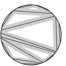
Figure 6: Illlustration of the proof of lemma 7.1: The chords $[x_{i}y_{i}]$ have to lie in the shaded part of the figure.

Let us turn to the proof of Theorem 1.4. We fix $\varepsilon>0$ and $\delta\in\,]0,1/2[$.

We use the genealogical structure of fragments as described in the beginning of the proof of Theorem 5.4. We first observe that we may fix an integer $m$ sufficiently large such that with probability at least $1-\delta$ all the fragments $R_{u}$ for $u\in\{0,1\}^{m}$ have mass less than $\varepsilon/2\pi$. Then, using Lemma 5.5, or rather the proof of this lemma, we can choose an integer $M\geq m$ large enough so that the following holds with probability greater than $1-\delta$: for every $u\in\{0,1\}^{M}$, there exists an integer $j(u)\in\{m,\ldots,M\}$ such that the fragment $R_{[u]_{j(u)}}$ has at most 3 ends.

From now on, we argue on the set where the preceding property holds and where all the fragments $R_{u}$ for $u\in\{0,1\}^{m}$ have mass less than $\varepsilon/2\pi$. For every $u\in\{0,1\}^{M}$, we choose the integer $j(u)$ as small as possible and set $v(u)=[u]_{j(u)}$ to simplify notation. Then, if $u,u^{\prime}\in\{0,1\}^{M}$, the fragments $R_{v(u)}$ and $R_{v(u^{\prime})}$ are either disjoint or equal. From this property, we easily get that there exists a figela $L^{*}$ whose fragments are the sets $R_{v(u)}$, $u\in\{0,1\}^{M}$. By construction, $L^{*}$ satisfies the assumptions of Lemma 7.1. Consequently, every chord appearing in the figela process lies within distance at most $\varepsilon$ from a chord of $L^{*}$.

For a given value of the integer $n\geq 3$, consider now the discrete triangulation $\Lambda_{n}$ of Section 1, such that feet of chords belong to the set of $n$th roots of unity, and recall the recursive construction of $\Lambda_{n}$. In this model we can introduce a labelling of fragments analogous to what we did in the continuous setting. For instance, $R^{n}_{0}$ and $R^{n}_{1}$ will be the fragments created by the first chord, ordered in a random way. Then we look for the first chord that falls in $R_{0}$ (if any) and call $R^{n}_{00}$ and $R^{n}_{01}$ the new fragments created by this chord, and so on. In this way we get a collection $(R^{n}_{u})_{u\in{\mathbb{T}}^{(n)}}$, which is indexed by a random finite subtree ${\mathbb{T}}^{(n)}$ of $\mathbb{T}$. It is easy to verify that, for every integer $p\geq 0$, ${\mathbb{P}}[\mathbb{T}_{p}\subset{\mathbb{T}}^{(n)}]$ tends to $1$ as $n\to\infty$.

For every $u\in\mathbb{T}$, write $x_{u}$ and $y_{u}$ for the feet of the first chord that will split $R_{u}$ (again ordered in a random way). Introduce a similar notation $x^{n}_{u}$ and $y^{n}_{u}$ in the discrete setting [then of course $x^{n}_{u}$ and $y^{n}_{u}$ are only defined when $u\in\mathbb{T}^{(n)}$ and $u$ is not a leaf of $\mathbb{T}^{(n)}$]. Since feet of chords are chosen recursively uniformly over possible choices, both in the discrete and in the continuous setting, it should be clear that, for every integer $p\geq 0$,

$$((x^{n}_{u},y^{n}_{u}))_{u\in\mathbb{T}_{p}}\stackrel{{\scriptstyle(d)}}{{\mathop{\longrightarrow}\limits_{n\to\infty}}}((x_{u},y_{u}))_{u\in\mathbb{T}_{p}}.$$ (33)

We apply this convergence with $p=M$. Using the Skorokhod representation theorem, we may assume that the preceding convergence holds almost surely. Then almost surely for $n$ sufficiently large, every chord of the figela $L^{*}$ (which must be of the form $[x_{u}y_{u}]$ for some $u\in\mathbb{T}_{M}$) lies within distance at most $\varepsilon$ from a chord of $\Lambda_{n}$. Recalling the beginning of the proof, we see that, on an event of probability at least $1-2\delta$, every chord appearing in the figela process lies within distance $2\varepsilon$ from a chord of $\Lambda_{n}$, for all $n$ sufficiently large.

We still need to prove the converse: We argue on the same event of probability at least $1-2\delta$ and verify that, for $n$ sufficiently large, every chord of $\Lambda_{n}$ lies within distance $2\varepsilon$ from the set $L_{\infty}$. To this end, we use a symmetric argument. Assuming that $n$ is large enough so that $\mathbb{T}_{M}\subset{\mathbb{T}}^{(n)}$, we let $\Lambda^{*}_{n}$ be the figela whose fragments are the sets $R^{n}_{v(u)}$, $u\in\{0,1\}^{M}$. The (almost sure) convergence (33) guarantees that every chord of the figela $L^{*}$ is the limit as $n\to\infty$ of the corresponding chord of $\Lambda^{*}_{n}$. It follows that, for $n$ sufficiently large, $\Lambda^{*}_{n}$ satisfies the assumptions of Lemma 7.1, and thus every chord of $\Lambda_{n}$ lies within distance at most $\varepsilon$ from a chord of $\Lambda^{*}_{n}$. Taking $n$ even larger if necessary, we get that every chord of $\Lambda_{n}$ lies within distance at most $2\varepsilon$ from a chord of $L^{*}$. This completes the proof of the first assertion of Theorem 1.4.

The second assertion is proved in a similar manner. Plainly, a uniformly distributed random permutation of $\{1,2,\ldots,n\}$ can be generated by first choosing $\sigma(1)$ uniformly over $\{1,\ldots,n\}$, then $\sigma(2)$ uniformly over $\{1,\ldots,n\}\setminus\{\sigma(1)\}$, and so on. From this simple remark, we see that the analogue of the convergence (33) still holds for the feet of chords of the figela $\widetilde{\Lambda}_{n}$. The remaining part of the argument goes through without change.

8 Extensions and comments

8.1 Case $\alpha=0$

Recall from Theorem 3.13(iv) the definition of $\mathscr{H}_{0}(x)$ as the almost sure limit of $e^{-t/3}H_{S_{0}(t)}(1,x)$ as $t\to\infty$. Note that $\mathscr{H}_{0}(x)$ is an analogue in the homogenous case $\alpha=0$ of $\mathscr{M}_{\infty}(x)$. In a way similar to what we did for $\mathscr{M}_{\infty}(x)$, one can verify that $\mathbb{E}[\mathscr{H}_{0}(x)^{p}]<\infty$ for every real $p\geq 1$, and derive integral equations for the moments $h_{p}(r)=\mathbb{E}[\mathscr{H}_{0}(e^{2i\pi r})^{p}]$, for $0\leq r\leq 1$. In the case $p=1$ we get

$$\frac{4}{3}h_{1}(r)=\int_{0}^{r}du\biggl{(}\frac{1-r}{1-u}\biggr{)}^{2}\frac{2h_{1}(u)}{1-u}+\int_{r}^{1}du\biggl{(}\frac{r}{u}\biggr{)}^{2}\frac{2h_{1}(u)}{u}.$$

By differentiating this equation three times with respect to the variable $r$ we get

$$\frac{2}{3}h_{1}^{\prime\prime\prime}(r)=h_{1}^{\prime\prime}(r)\biggl{(}\frac{1}{1-r}-\frac{1}{r}\biggr{)},$$

leading to the explicit formula

$$h_{1}(r)=\frac{8}{\pi}\sqrt{r(1-r)}.$$

For higher values of $p$, we get the following bounds.

Proposition 8.1

For every integer $p\geq 1$ and every $\varepsilon>0$, there exists a constant $K$ such that for every $r\in[0,1]$,

$$h_{p}(r)\leq K\bigl{(}r(1-r)\bigr{)}^{{2p/(p+3)}-\varepsilon}.$$

We omit the proof, which uses arguments similar to the proof of Proposition 4.1. The bounds of Proposition 8.1 are not sharp. Still they are good enough to apply Kolmogorov’s continuity criterion in order to get a continuous modification of the process $(\mathscr{H}_{0}(x))_{x\in\mathbb{S}_{1}}$.

8.2 Recursive self-similarity

Set $Z_{t}=\mathscr{M}_{\infty}(e^{2i\pi t})$ for every $t\in[0,1]$. A slightly more precise version of Proposition 5.1 shows that the process $(Z_{t})_{t\in[0,1]}$ satisfies the following remarkable self-similarity property. Let $Z^{\prime}$ and $Z^{\prime\prime}$ be two independent copies of $Z$ and let $(U_{1},U_{2})$ be distributed according to the density $2{\mathbf{1}}_{\{0<u_{1}<u_{2}<1\}}$ and independent of the pair $(Z,Z^{\prime})$. Then the process $(\widetilde{Z}_{t})_{t\in[0,1]}$ defined by

$$\widetilde{Z}_{t}=\cases{\displaystyle\bigl{(}1-(U_{2}-U_{1})\bigr{)}^{\beta^{*}}Z^{\prime}_{t/(1-(U_{2}-U_{1}))},\vspace*{1pt}\cr\qquad\mbox{if }0\leq t\leq U_{1},\vspace*{3pt}\cr\displaystyle\bigl{(}1-(U_{2}-U_{1})\bigr{)}^{\beta^{*}}Z^{\prime}_{U_{1}/(1-(U_{2}-U_{1}))}+(U_{2}-U_{1})^{\beta^{*}}Z^{\prime\prime}_{(t-U_{1})/(U_{2}-U_{1})},\vspace*{1pt}\cr\qquad\mbox{ if }U_{1}\leq t\leq U_{2},\vspace*{3pt}\cr\displaystyle\bigl{(}1-(U_{2}-U_{1})\bigr{)}^{\beta^{*}}Z^{\prime}_{(t-(U_{2}-U_{1}))/(1-(U_{2}-U_{1}))},\vspace*{1pt}\cr\qquad\mbox{ if }U_{2}\leq t\leq 1,}$$

has the same distribution as $(Z_{t})_{t\in[0,1]}$.

Informally, this means that we can write a decomposition of $Z$ in two pieces according to the following device. Throw two independent uniform points $U_{1}$ and $U_{2}$ in $[0,1]$. Condition on the event $U_{1}<U_{2}$ and set $M=1-(U_{2}-U_{1})$. Then start from a (scaled) copy of $Z$ of duration $[0,M]$ and “insert” at time $U_{1}$ another independent scaled copy of $Z$ of duration $1-M$. Then the resulting random function has the same distribution as $Z$.

In Ald94a , Aldous describes such a decomposition in three pieces for the Brownian excursion, which is closely related to the random geodesic lamination $L_{\mathbf{e}}$ of Theorem 2.6. Aldous also conjectures that there cannot exist a decomposition of the Brownian excursion in two pieces of the type described above.

It would be interesting to know whether the preceding decomposition of $Z$ (along with some regularity properties) characterizes the distribution of $Z$ up to trivial scaling constants. One may also ask whether the scaling exponent $\beta^{*}$ is the only one for which there can exist such a decomposition in two pieces.

References

- (1) {barticle}[mr] \bauthor\bsnmAldous, \bfnmDavid\binitsD. (\byear1994). \btitleRecursive self-similarity for random trees, random triangulations and Brownian excursion. \bjournalAnn. Probab. \bvolume22 \bpages527–545. \bidmr=1288122 \endbibitem
- (2) {barticle}[mr] \bauthor\bsnmAldous, \bfnmDavid\binitsD. (\byear1994). \btitleTriangulating the circle, at random. \bjournalAmer. Math. Monthly \bvolume101 \bpages223–233. \biddoi=10.2307/2975599, mr=1264002 \endbibitem
- (3) {bbook}[mr] \bauthor\bsnmAthreya, \bfnmKrishna B.\binitsK. B. and \bauthor\bsnmNey, \bfnmPeter E.\binitsP. E. (\byear1972). \btitleBranching Processes. \bpublisherSpringer, \baddressNew York. \bidmr=0373040 \endbibitem
- (4) {bbook}[mr] \bauthor\bsnmBertoin, \bfnmJean\binitsJ. (\byear2006). \btitleRandom Fragmentation and Coagulation Processes. \bseriesCambridge Studies in Advanced Mathematics \bvolume102. \bpublisherCambridge Univ. Press, \baddressCambridge. \biddoi=10.1017/CBO9780511617768, mr=2253162 \endbibitem
- (5) {barticle}[mr] \bauthor\bsnmBertoin, \bfnmJean\binitsJ. and \bauthor\bsnmGnedin, \bfnmAlexander V.\binitsA. V. (\byear2004). \btitleAsymptotic laws for nonconservative self-similar fragmentations. \bjournalElectron. J. Probab. \bvolume9 \bpages575–593 (electronic). \bidmr=2080610 \endbibitem
- (6) {bincollection}[mr] \bauthor\bsnmBonahon, \bfnmFrancis\binitsF. (\byear2001). \btitleGeodesic laminations on surfaces. In \bbooktitleLaminations and Foliations in Dynamics, Geometry and Topology (Stony Brook, NY, 1998). \bseriesContemp. Math. \bvolume269 \bpages1–37. \bpublisherAmer. Math. Soc., \baddressProvidence, RI. \bidmr=1810534 \endbibitem
- (7) {barticle}[mr] \bauthor\bsnmBrennan, \bfnmMichael D.\binitsM. D. and \bauthor\bsnmDurrett, \bfnmRichard\binitsR. (\byear1986). \btitleSplitting intervals. \bjournalAnn. Probab. \bvolume14 \bpages1024–1036. \bidmr=0841602 \endbibitem
- (8) {barticle}[mr] \bauthor\bsnmBrennan, \bfnmMichael D.\binitsM. D. and \bauthor\bsnmDurrett, \bfnmRichard\binitsR. (\byear1987). \btitleSplitting intervals. II. Limit laws for lengths. \bjournalProbab. Theory Related Fields \bvolume75 \bpages109–127. \biddoi=10.1007/BF00320085, mr=0879556 \endbibitem
- (9) {bmisc}[auto:SpringerTagBib—2010-11-18—09:18:59] \bauthor\bsnmDavid, \bfnmF.\binitsF., \bauthor\bsnmDukes, \bfnmW. M. B.\binitsW. M. B., \bauthor\bsnmJonsson, \bfnmT.\binitsT. and \bauthor\bsnmStefánsson, \bfnmS. Ö.\binitsS. Ö. (\byear2009). \bhowpublishedRandom tree growth by vertex splitting. J. Stat. Mech. P04009. \endbibitem
- (10) {bmisc}[auto:SpringerTagBib—2010-11-18—09:18:59] \bauthor\bsnmDavid, \bfnmF.\binitsF., \bauthor\bsnmHagendorf, \bfnmC.\binitsC. and \bauthor\bsnmWiese, \bfnmK. J.\binitsK. J. (\byear2008). \bhowpublishedA growth model for RNA secondary structures. J. Stat. Mech. P04008. \endbibitem
- (11) {barticle}[mr] \bauthor\bsnmDevroye, \bfnmL.\binitsL., \bauthor\bsnmFlajolet, \bfnmP.\binitsP., \bauthor\bsnmHurtado, \bfnmF.\binitsF., \bauthor\bsnmNoy, \bfnmM.\binitsM. and \bauthor\bsnmSteiger, \bfnmW.\binitsW. (\byear1999). \btitleProperties of random triangulations and trees. \bjournalDiscrete Comput. Geom. \bvolume22 \bpages105–117. \biddoi=10.1007/PL00009444, mr=1692686 \endbibitem
- (12) {barticle}[mr] \bauthor\bsnmDuquesne, \bfnmThomas\binitsT. and \bauthor\bsnmLe Gall, \bfnmJean-François\binitsJ.-F. (\byear2005). \btitleProbabilistic and fractal aspects of Lévy trees. \bjournalProbab. Theory Related Fields \bvolume131 \bpages553–603. \biddoi=10.1007/s00440-004-0385-4, mr=2147221 \endbibitem
- (13) {bbook}[mr] \bauthor\bsnmEvans, \bfnmSteven N.\binitsS. N. (\byear2008). \btitleProbability and Real Trees. \bseriesLecture Notes in Math. \bvolume1920. \bpublisherSpringer, \baddressBerlin. \biddoi=10.1007/978-3-540-74798-7, mr=2351587 \endbibitem
- (14) {barticle}[mr] \bauthor\bsnmLe Gall, \bfnmJean-François\binitsJ.-F. and \bauthor\bsnmPaulin, \bfnmFrédéric\binitsF. (\byear2008). \btitleScaling limits of bipartite planar maps are homeomorphic to the 2-sphere. \bjournalGeom. Funct. Anal. \bvolume18 \bpages893–918. \biddoi=10.1007/s00039-008-0671-x, mr=2438999 \endbibitem
- (15) {barticle}[mr] \bauthor\bsnmLiu, \bfnmQuansheng\binitsQ. (\byear1997). \btitleSur une équation fonctionnelle et ses applications: Une extension du théorème de Kesten-Stigum concernant des processus de branchement. \bjournalAdv. in Appl. Probab. \bvolume29 \bpages353–373. \biddoi=10.2307/1428007, mr=1450934 \endbibitem
- (16) {bmisc}[auto:SpringerTagBib—2010-11-18—09:18:59] \bauthor\bsnmMüller, \bfnmM.\binitsM. (\byear2003). \bhowpublishedRepliement d’hétéropolymères. Ph.D. thesis, Université Paris-Sud. Available at: http://users.ictp.it/~markusm/PhDThesis.pdf. \endbibitem
- (17) {bbook}[mr] \bauthor\bsnmRevuz, \bfnmDaniel\binitsD. and \bauthor\bsnmYor, \bfnmMarc\binitsM. (\byear1999). \btitleContinuous Martingales and Brownian Motion, \bedition3rd ed. \bseriesGrundlehren der Mathematischen Wissenschaften [Fundamental Principles of Mathematical Sciences] \bvolume293. \bpublisherSpringer, \baddressBerlin. \bidmr=1725357 \endbibitem
- (18) {barticle}[mr] \bauthor\bsnmSleator, \bfnmDaniel D.\binitsD. D., \bauthor\bsnmTarjan, \bfnmRobert E.\binitsR. E. and \bauthor\bsnmThurston, \bfnmWilliam P.\binitsW. P. (\byear1988). \btitleRotation distance, triangulations, and hyperbolic geometry. \bjournalJ. Amer. Math. Soc. \bvolume1 \bpages647–681. \biddoi=10.2307/1990951, mr=0928904 \endbibitem