We explored the effects of relative motion on the excitation of surface–plasmon–polariton (SPP) waves guided by the planar interface of a metal film and a dielectric slab, both materials being isotropic and homogeneous. Electromagnetic phasors in moving and non–moving reference frames were related directly using the corresponding Lorentz transformations. Our numerical studies revealed that, in the case of a uniformly moving dielectric slab, the angle of incidence for SPP-wave excitation is highly sensitive to (i) the ratio $\beta$ of the speed of motion to speed of light in free space and (ii) the direction of motion. When the direction of motion is parallel to the plane of incidence, the SPP wave is excited by $p$-polarized (but not $s$-polarized) incident plane waves for low and moderate values of $\beta$, while at higher values of $\beta$ the total reflection regime breaks down. When the direction of motion is perpendicular to the plane of incidence, the SPP wave is excited by $p$-polarized incident plane waves for low values of $\beta$, but $s$-polarized incident plane waves at moderate values of $\beta$, while at higher values of $\beta$ the SPP wave is not excited. In the case of a uniformly moving metal film, the sensitivity to $\beta$ and the direction of motion is less obvious.

Keywords: surface plasmon polariton, Lorentz transformation, modified Kretschmann configuration

1 Introduction

In quantum mechanical terms, a surface plasmon–polariton (SPP) is a quasiparticle. Created by the interaction of photons in a dielectric material and electrons in a metal, a SPP travels along the interface of the metal and the dielectric material [1]. In classical terms, a SPP wave propagates guided by the interface with an amplitude that decreases exponentially with distance from the interface. Over the past few decades, SPP waves have been widely investigated, in part because of the opportunities that they present for optical sensing applications [2, 3]. Most published research deals with SPP waves guided by the interface of a metal with an isotropic dielectric material, both homogeneous [4, 5, 6]. Guidance by the interface of a metal with an anisotropic dielectric material has also been examined [7, 8, 9, 10, 11, 12]. The interface of a metal with a periodically nonhomogeneous and anisotropic dielectric material has recently been found to support more than one mode of SPP-wave propagation at a fixed frequency [13, 14, 15].

In this communication, we address a fundamental issue: the effect of relative uniform motion on SPP-wave propagation guided by the planar interface of a metal and a dielectric material, both isotropic and homogeneous. This is done using a modification [16] of the standard Kretschmann configuration [4], as detailed in Sec. 2. Electromagnetic phasors in moving and non–moving (laboratory) inertial reference frames are related directly using the corresponding Lorentz transformations [17, 18], and not the Minkowski constitutive relations [19, Chap. 8]. Section 3 provides numerical results, and some remarks in Sec. 4 close this communication.

As regards notation, vectors and matrixes are written in boldface, with the $\hat{}$ symbol denoting a unit vector. Square brackets enclose 2–, 4– and 6–vectors, as well as 2$\times$2, 4$\times$4 and 6$\times$6 matrixes. Double underlining indicates a 3$\times$3 dyadic, with the identity dyadic $\underline{\underline{I}}=\hat{{\bf x}}\,\hat{{\bf x}}+\hat{{\bf y}}\,\hat{{\bf y}}+\hat{{\bf z}}\,\hat{{\bf z}}$ and the null dyadic being $\underline{\underline{0}}$. The permittivity and permeability of free space are denoted by $\epsilon_{0}$ and $\mu_{0}$; the free–space wavenumber at angular frequency $\omega$ is $k_{0}=\omega\sqrt{\epsilon_{0}\mu_{0}}$; and $c_{0}=\omega/k_{0}$.

2 Analysis

The partition of space into four distinct layers provides the backdrop for our analysis:

• the half–space $z<0$ is occupied by a dielectric material with relative permittivity scalar $\epsilon_{i}$ with respect to the inertial reference frame $\Pi$, which is the laboratory frame;

• a thin metal film of relative permittivity scalar $\epsilon_{m}$ with respect to the inertial reference frame $\Pi$ fills the layer $0<z<L_{m}$;

• a dielectric slab of relative permittivity scalar $\epsilon^{\prime}_{d}$ with respect to the inertial reference frame $\Pi^{\prime}$ fills the layer $L_{m}<z<L_{\Sigma}$; and

• the half–space $z>L_{\Sigma}$ is occupied by a dielectric material with relative permittivity scalar $\epsilon_{t}$ with respect to the inertial reference frame $\Pi$.

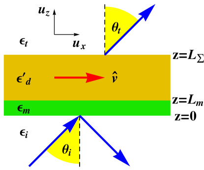
Figure 1: A schematic depiction of the modified Kretschmann configuration under investigation. A plane wave is incident upon a metal film occupying $0<z<L_{m}$. The region $L_{m}<z<L_{\Sigma}$ is filled by a dielectric slab which moves at constant velocity in the direction of $\hat{{\bf v}}$.

All four materials are homogeneous and their relative permittivity scalars are frequency-dependent in their respective co-moving inertial reference frames. Dissipation is small enough to be ignored in both materials occupying the two half–spaces as well as in the dielectric slab. The reference frame $\Pi^{\prime}$ moves at uniform velocity ${\bf v}=v\hat{{\bf v}}$, in the $xy$ plane, with respect to the laboratory frame $\Pi$. This setup, schematically illustrated in Fig. 1 for the case $\hat{{\bf v}}=\hat{{\bf x}}$, represents a modification [16] of the standard Kretschmann configuration [4], suitable for launching SPP waves guided by the planar interface of the metal film and the dielectric slab; i.e., along $z=L_{m}$.

Suppose that an arbitrarily polarized plane wave in the half–space $z<0$ is directed towards the metal film. Its wavevector lies in the $xz$ plane, making an angle $\theta_{i}\in\left[0,\pi/2\right)$ to the $+z$ axis, in the laboratory frame $\Pi$. In consequence, a reflected plane wave is generated in the half–space $z<0$ along with a transmitted plane wave in the half–space $z>L_{\Sigma}$. In the laboratory frame, the total electric field phasor in the half–space $z<0$ may be written as

$${\bf E}({\bf r},\omega) = \big{\{}\left[\,a_{s}{\bf u}_{y}+a_{p}{\bf p}_{+}(\theta_{i})\right]\exp\left(ik_{0}\sqrt{\epsilon_{i}}\,z\cos\theta_{i}\right)+\left[\,r_{s}{\bf u}_{y}+r_{p}{\bf p}_{-}(\theta_{i})\right]\exp\left(-ik_{0}\sqrt{\epsilon_{i}}\,z\cos\theta_{i}\right)\big{\}}$$ (1)

$$\times\exp\left(i\kappa x\right),\qquad z<0,$$

whereas that in the half–space $z>L_{\Sigma}$ may be written as

$${\bf E}({\bf r},\omega)=\left[\,t_{s}{\bf u}_{y}+t_{p}{\bf p}_{+}(\theta_{t})\,\right]\exp\left[ik_{0}\sqrt{\epsilon_{t}}\left(z-L_{\Sigma}\right)\cos\theta_{t}\right]\,\exp\left(i\kappa x\right),\qquad z>L_{\Sigma}.$$ (2)

Here ${\bf p}_{\pm}(\theta)=\mp{\bf u}_{x}\cos\theta+{\bf u}_{z}\sin\theta$, $\kappa=k_{0}\sqrt{\epsilon_{i}}\,\sin\theta_{i}$ and the angle of transmission $\theta_{t}$ in frame $\Pi$ satisfies

$$\sqrt{\epsilon_{i}}\,\sin\theta_{i}=\sqrt{\epsilon_{t}}\,\sin\theta_{t}.$$ (3)

Our task is to relate the complex–valued reflection and transmission amplitudes—namely $r_{s}$, $r_{p}$, $t_{s}$ and $t_{p}$—to the corresponding amplitudes $a_{s}$ and $a_{p}$ of the $s$- and $p$-polarized components of the incident plane wave.

For later use, we note that the wavevector

$${\bf k}_{i}=\kappa\,\hat{{\bf x}}+k_{0}\sqrt{\epsilon_{i}}\,\cos\theta_{i}\,\hat{{\bf z}},\qquad z<0,$$ (4)

of the incident plane wave in frame $\Pi$ is related to its counterpart ${\bf k}^{\prime}_{i}$ in frame $\Pi^{\prime}$ by the Lorentz transformation [19, 20]

$${\bf k}_{i}=\displaystyle{\gamma\left({\bf k}^{\prime}_{i}\cdot\hat{{\bf v}}+\frac{\omega^{\prime}v}{c_{0}^{2}}\right)\hat{{\bf v}}+\left(\,\underline{\underline{I}}-\hat{{\bf v}}\,\hat{{\bf v}}\right)\cdot{\bf k}^{\prime}_{i}},$$ (5)

where the scalar parameters

$$\gamma=\frac{1}{\sqrt{1-\beta^{2}}},\qquad\beta=\frac{v}{c_{0}}.$$ (6)

The angular frequencies in the two frames are related per

$$\omega=\displaystyle{\gamma\left(\omega^{\prime}+{\bf k}^{\prime}_{i}\cdot{\bf v}\right)}.$$ (7)

In the metal film, the electric and magnetic field phasors with respect to the laboratory frame $\Pi$, namely ${\bf E}({\bf r},\omega)={\bf e}(z,\kappa,\omega)\,\exp\left(i\kappa x\right)$ and ${\bf H}({\bf r},\omega)={\bf h}(z,\kappa,\omega)\,\exp\left(i\kappa x\right)$, are related via the Maxwell curl postulates; thus,

$$\frac{d}{dz}\left[{\bf f}(z,\kappa,\omega)\right] = i\left[{\bf P}(\epsilon_{m},\kappa,\omega)\right]\,\left[{\bf f}(z,\kappa,\omega)\right],\qquad 0<z<L_{m},$$ (8)

where the 4–vector

$$\left[{\bf f}(z,\kappa,\omega)\right]=\left[\begin{array}[]{c}{\bf e}(z,\kappa,\omega)\cdot\hat{{\bf x}}\\ {\bf e}(z,\kappa,\omega)\cdot\hat{{\bf y}}\\ {\bf h}(z,\kappa,\omega)\cdot\hat{{\bf x}}\\ {\bf h}(z,\kappa,\omega)\cdot\hat{{\bf y}}\end{array}\right]$$ (9)

and the 4$\times$4 matrix

$$\left[{\bf P}(\epsilon,\kappa,\omega)\right]=\omega\left[\begin{array}[]{cccc}0&0&0&\mu_{0}-\frac{\kappa^{2}}{\omega^{2}\epsilon_{0}\epsilon}\\ 0&0&-\mu_{0}&0\\ 0&\frac{\kappa^{2}}{\omega^{2}\mu_{0}}-\epsilon_{0}\epsilon&0&0\\ \epsilon_{0}\epsilon&0&0&0\end{array}\right].$$ (14)

The solution to the matrix ordinary differential equation (8) is conveniently stated as

$$\left[{\bf f}(L_{m},\kappa,\omega)\right]=\left[{\bf M}(\epsilon_{m},L_{m},\kappa,\omega)\right]\left[{\bf f}(0,\kappa,\omega)\right],$$ (16)

where the transfer matrix

$$\left[{\bf M}(\epsilon_{m},L_{m},\kappa,\omega)\right]=\exp\left\{iL_{m}\left[{\bf P}(\epsilon_{m},\kappa,\omega)\right]\right\}.$$ (17)

In a similar fashion, the electric and magnetic field phasors with respect to frame $\Pi^{\prime}$, namely ${\bf E}^{\prime}({\bf r}^{\prime},\omega^{\prime})={\bf e}^{\prime}(z,\kappa^{\prime},\omega^{\prime})\,\exp\left(i\kappa^{\prime}x^{\prime}\right)$ and ${\bf H}^{\prime}({\bf r}^{\prime},\omega^{\prime})={\bf h}^{\prime}(z,\kappa^{\prime},\omega^{\prime})\,\exp\left(i\kappa^{\prime}x^{\prime}\right)$, satisfy the matrix ordinary differential equation

$$\frac{d}{dz}\left[{\bf f}^{\prime}(z,\kappa^{\prime},\omega^{\prime})\right] = i\left[{\bf P}(\epsilon^{\prime}_{d},\kappa^{\prime},\omega^{\prime})\right]\,\left[{\bf f}^{\prime}(z,\kappa^{\prime},\omega^{\prime})\right],\qquad L_{m}<z<L_{\Sigma}$$ (18)

in the dielectric slab, where the 4–vector

$$\left[{\bf f}^{\prime}(z,\kappa^{\prime},\omega^{\prime})\right]=\left[\begin{array}[]{c}{\bf e}^{\prime}(z,\kappa^{\prime},\omega^{\prime})\cdot\hat{{\bf x}}\\ {\bf e}^{\prime}(z,\kappa^{\prime},\omega^{\prime})\cdot\hat{{\bf y}}\\ {\bf h}^{\prime}(z,\kappa^{\prime},\omega^{\prime})\cdot\hat{{\bf x}}\\ {\bf h}^{\prime}(z,\kappa^{\prime},\omega^{\prime})\cdot\hat{{\bf y}}\end{array}\right],$$ (19)

the angular frequency $\omega^{\prime}$ is specified by (7) and $\kappa^{\prime}={\bf k}^{\prime}_{i}\cdot\hat{{\bf x}}$ with ${\bf k}^{\prime}_{i}$ being specified by (5). The solution to the matrix ordinary differential equation (18) is conveniently stated as

$$\left[{\bf f}^{\prime}(L_{\Sigma},\kappa^{\prime},\omega^{\prime})\right]=\left[{\bf M}(\epsilon^{\prime}_{d},L_{\Sigma}-L_{m},\kappa^{\prime},\omega^{\prime})\right]\left[{\bf f}^{\prime}(L_{m},\kappa^{\prime},\omega^{\prime})\right].$$ (20)

We now seek to express the solution (20) in terms of the field phasors in the laboratory frame $\Pi$. Using the fact that the $z$ components of ${\bf e}^{\prime}(z,\kappa^{\prime},\omega^{\prime})$ and ${\bf h}^{\prime}(z,\kappa^{\prime},\omega^{\prime})$ are related via the Maxwell curl postulates per

$$\left.\begin{array}[]{l}{\bf e}^{\prime}(z,\kappa^{\prime},\omega^{\prime})\cdot\hat{{\bf z}}=-\displaystyle{\frac{\kappa^{\prime}}{\omega^{\prime}\epsilon_{0}\epsilon^{\prime}_{d}}\,{\bf h}^{\prime}(z,\kappa^{\prime},\omega^{\prime})\cdot\hat{{\bf y}}\vspace{4pt}}\\ {\bf h}^{\prime}(z,\kappa^{\prime},\omega^{\prime})\cdot\hat{{\bf z}}=\displaystyle{\frac{\kappa^{\prime}}{\omega^{\prime}\mu_{0}}\,{\bf e}^{\prime}(z,\kappa^{\prime},\omega^{\prime})\cdot\hat{{\bf y}}}\end{array}\right\},$$ (21)

we introduce the 6–vector extension of $\left[{\bf f}^{\prime}(z,\kappa^{\prime},\omega^{\prime})\right]$, namely

$$\left[\tilde{{\bf f}}^{\prime}(z,\kappa^{\prime},\omega^{\prime})\right]=\left[\begin{array}[]{c}{\bf e}^{\prime}(z,\kappa^{\prime},\omega^{\prime})\cdot\hat{{\bf x}}\\ {\bf e}^{\prime}(z,\kappa^{\prime},\omega^{\prime})\cdot\hat{{\bf y}}\\ {\bf e}^{\prime}(z,\kappa^{\prime},\omega^{\prime})\cdot\hat{{\bf z}}\\ {\bf h}^{\prime}(z,\kappa^{\prime},\omega^{\prime})\cdot\hat{{\bf x}}\\ {\bf h}^{\prime}(z,\kappa^{\prime},\omega^{\prime})\cdot\hat{{\bf y}}\\ {\bf h}^{\prime}(z,\kappa^{\prime},\omega^{\prime})\cdot\hat{{\bf z}}\end{array}\right],$$ (22)

and the 6$\times$6 matrix extension of $\left[{\bf M}(\epsilon^{\prime}_{d},L_{\Sigma}-L_{m},\kappa^{\prime},\omega^{\prime})\right]$, namely $\left[\tilde{{\bf M}}(\epsilon^{\prime}_{d},L_{\Sigma}-L_{m},\kappa^{\prime},\omega^{\prime})\right]$, with components

$$\left[\tilde{{\bf M}}(\epsilon^{\prime}_{d},L_{\Sigma}-L_{m},\kappa^{\prime},\omega^{\prime})\right]_{\tilde{p}\tilde{q}}=\left[{\bf M}(\epsilon^{\prime}_{d},L_{\Sigma}-L_{m},\kappa^{\prime},\omega^{\prime})\right]_{pq},\qquad\tilde{p},\tilde{q}\in\left\{1,2,4,5\right\};\quad p,q\in\left\{1,2,3,4\right\};$$

(23)

$$\left[\tilde{{\bf M}}(\epsilon^{\prime}_{d},L_{\Sigma}-L_{m},\kappa^{\prime},\omega^{\prime})\right]_{3\tilde{q}}=-\displaystyle{\frac{\kappa^{\prime}}{\omega^{\prime}\epsilon_{0}\epsilon^{\prime}_{d}}\,\left[{\bf M}(\epsilon^{\prime}_{d},L_{\Sigma}-L_{m},\kappa^{\prime},\omega^{\prime})\right]_{4q},\qquad\tilde{q}\in\left\{1,2,4,5\right\};\quad q\in\left\{1,2,3,4\right\};}$$

(24)

$$\left[\tilde{{\bf M}}(\epsilon^{\prime}_{d},L_{\Sigma}-L_{m},\kappa^{\prime},\omega^{\prime})\right]_{6\tilde{q}}=\displaystyle{\frac{\kappa^{\prime}}{\omega^{\prime}\mu_{0}}\,\left[{\bf M}(\epsilon^{\prime}_{d},L_{\Sigma}-L_{m},\kappa^{\prime},\omega^{\prime})\right]_{2q},\qquad\tilde{q}\in\left\{1,2,4,5\right\};\quad q\in\left\{1,2,3,4\right\};}$$

(25)

$$\left[\tilde{{\bf M}}(\epsilon^{\prime}_{d},L_{\Sigma}-L_{m},\kappa^{\prime},\omega^{\prime})\right]_{\tilde{p}\tilde{q}}=0,\qquad\tilde{p},\tilde{q}\in\left\{3,6\right\}.$$ (26)

Thus, the solution (20) may be extended as

$$\left[\tilde{{\bf f}}^{\prime}(L_{\Sigma},\kappa^{\prime},\omega^{\prime})\right]=\left[\tilde{{\bf M}}(\epsilon^{\prime}_{d},L_{\Sigma}-L_{m},\kappa^{\prime},\omega^{\prime})\right]\left[\tilde{{\bf f}}^{\prime}(L_{m},\kappa^{\prime},\omega^{\prime})\right].$$ (27)

Now in the dielectric slab the electromagnetic phasors in frames $\Pi$ and $\Pi^{\prime}$ are related by the Lorentz transformations [20]

$$\left.\begin{array}[]{l}{\bf e}(z,\kappa,\omega)=\underline{\underline{A}}_{\,d}\cdot{\bf e}^{\prime}(z,\kappa^{\prime},\omega^{\prime})\\[5.0pt] {\bf h}(z,\kappa,\omega)=\underline{\underline{A}}_{\,d}\cdot{\bf h}^{\prime}(z,\kappa^{\prime},\omega^{\prime})\end{array}\right\},\qquad L_{m}<z<L_{\Sigma},$$ (28)

where the 3$\times$3 dyadic

$$\underline{\underline{A}}_{\,d}=\left(1-\gamma\right)\hat{{\bf v}}\,\hat{{\bf v}}+\gamma\underline{\underline{I}}-\frac{\gamma}{\omega^{\prime}}\left({\bf v}\times\underline{\underline{I}}\,\right)\cdot\left({\bf k}^{\prime}_{d}\times\underline{\underline{I}}\,\right),$$ (29)

with

$${\bf k}^{\prime}_{d}=\kappa^{\prime}\hat{{\bf x}}^{\prime}+\sqrt{\left(\omega^{\prime}\right)^{2}\epsilon_{0}\epsilon^{\prime}_{d}\mu_{0}-\left(\kappa^{\prime}\right)^{2}}\;\;\hat{{\bf z}},\qquad L_{m}<z<L_{\Sigma}.$$ (30)

Thus, (27) leads to

$$\left[\tilde{{\bf f}}(L_{\Sigma},\kappa,\omega)\right]=\left[\tilde{{\bf N}}(\epsilon^{\prime}_{d},L_{\Sigma}-L_{m},\kappa,\omega)\right]\left[\tilde{{\bf f}}(L_{m},\kappa,\omega)\right]$$ (31)

in the laboratory frame $\Pi$, with the 6$\times$6 matrix

$$\left[\tilde{{\bf N}}(\epsilon^{\prime}_{d},L_{\Sigma}-L_{m},\kappa,\omega)\right]=\left[\begin{array}[]{cc}\underline{\underline{A}}_{\,d}&\underline{\underline{0}}\vspace{4pt}\\ \underline{\underline{0}}&\underline{\underline{A}}_{\,d}\end{array}\right]^{-1}\left[\tilde{{\bf M}}(\epsilon^{\prime}_{d},L_{\Sigma}-L_{m},\kappa^{\prime},\omega^{\prime})\right]\left[\begin{array}[]{cc}\underline{\underline{A}}_{\,d}&\underline{\underline{0}}\vspace{4pt}\\ \underline{\underline{0}}&\underline{\underline{A}}_{\,d}\end{array}\right]$$ (32)

and the 6–vector

$$\left[\tilde{{\bf f}}(z,\kappa,\omega)\right]=\left[\begin{array}[]{c}{\bf e}(z,\kappa,\omega)\cdot\hat{{\bf x}}\\ {\bf e}(z,\kappa,\omega)\cdot\hat{{\bf y}}\\ {\bf e}(z,\kappa,\omega)\cdot\hat{{\bf z}}\\ {\bf h}(z,\kappa,\omega)\cdot\hat{{\bf x}}\\ {\bf h}(z,\kappa,\omega)\cdot\hat{{\bf y}}\\ {\bf h}(z,\kappa,\omega)\cdot\hat{{\bf z}}\end{array}\right].$$ (33)

Finally, the counterpart of (20) in the laboratory frame $\Pi$ emerges as

$$\left[{\bf f}(L_{\Sigma},\kappa,\omega)\right]=\left[{\bf N}(\epsilon^{\prime}_{d},L_{\Sigma}-L_{m},\kappa,\omega)\right]\left[{\bf f}(L_{m},\kappa,\omega)\right],$$ (34)

wherein the components of the 4$\times$4 matrix $\left[{\bf N}(\epsilon^{\prime}_{d},L_{\Sigma}-L_{m},\kappa,\omega)\right]$ are given by

$$\left[{\bf N}(\epsilon^{\prime}_{d},L_{\Sigma}-L_{m},\kappa,\omega)\right]_{pq}=\left[\tilde{{\bf N}}(\epsilon^{\prime}_{d},L_{\Sigma}-L_{m},\kappa,\omega)\right]_{\tilde{p}\tilde{q}},\qquad p,q\in\left\{1,2,3,4\right\};\quad\tilde{p},\tilde{q}\in\left\{1,2,4,5\right\}.$$

For later use, we introduce the 4$\times$4 matrix $\left[{\bf Q}(\epsilon^{\prime}_{d},\kappa,\omega)\right]$ via

$$\left[{\bf N}(\epsilon^{\prime}_{d},L_{\Sigma}-L_{m},\kappa,\omega)\right]=\exp\left\{i\left(L_{\Sigma}-L_{m}\right)\left[{\bf Q}(\epsilon^{\prime}_{d},\kappa,\omega)\right]\right\}.$$ (36)

The matrixes $\left[{\bf N}(\epsilon^{\prime}_{d},L_{\Sigma}-L_{m},\kappa,\omega)\right]$ and $\left[{\bf Q}(\epsilon^{\prime}_{d},\kappa,\omega)\right]$ have the same eigenvectors. The eigenvalues $\sigma_{\ell}$, $\ell\in\left\{1,2,3,4\right\}$, of $\left[{\bf N}(\epsilon^{\prime}_{d},L_{\Sigma}-L_{m},\kappa,\omega)\right]$ are related to the eigenvalues $\alpha_{\ell}$ of $\left[{\bf Q}(\epsilon^{\prime}_{d},\kappa,\omega)\right]$ as follows:

$$\alpha_{\ell}=\frac{\ln\sigma_{\ell}}{i\left(L_{\Sigma}-L_{m}\right)},\qquad\quad\ell\in\left\{1,2,3,4\right\}.$$ (37)

Upon combining the solutions (16) and (34), and invoking the boundary conditions on the tangential components of the electric and magnetic phasors at the planar interfaces, we arrive at the algebraic relation

$$\left[\begin{array}[]{c}t_{s}\\ t_{p}\\ 0\\ 0\end{array}\right] = \left[\,{\bf K}(\epsilon_{t},\theta_{t})\,\right]^{-1}\left[{\bf N}(\epsilon^{\prime}_{d},L_{\Sigma}-L_{m},\kappa,\omega)\right]\left[{\bf M}(\epsilon_{m},L_{m},\kappa,\omega)\right]\left[\,{\bf K}(\epsilon_{i},\theta_{i})\,\right]\left[\begin{array}[]{c}a_{s}\\ a_{p}\\ r_{s}\\ r_{p}\end{array}\right],$$ (46)

where the 4$\times$4 matrix

$$\left[\,{\bf K}(\epsilon,\theta)\,\right]=\left[\begin{array}[]{cccc}0&-\cos\theta&0&\cos\theta\\ 1&0&1&0\\ -\frac{\sqrt{\epsilon}\,\cos\theta}{\eta_{0}}&0&\frac{\sqrt{\epsilon}\,\cos\theta}{\eta_{0}}&0\\ 0&-\frac{\sqrt{\epsilon}}{\eta_{0}}&0&-\frac{\sqrt{\epsilon}}{\eta_{0}}\end{array}\right].$$ (51)

A straightforward manipulation of (46) yields

$$\left[\begin{array}[]{c}r_{s}\vspace{4pt}\\ r_{p}\end{array}\right]=\left[\begin{array}[]{cc}r_{ss}&r_{sp}\vspace{4pt}\\ r_{ps}&r_{pp}\end{array}\right]\left[\begin{array}[]{c}a_{s}\vspace{4pt}\\ a_{p}\end{array}\right]$$ (53)

and

$$\left[\begin{array}[]{c}t_{s}\vspace{4pt}\\ t_{p}\end{array}\right]=\left[\begin{array}[]{cc}t_{ss}&t_{sp}\vspace{4pt}\\ t_{ps}&t_{pp}\end{array}\right]\left[\begin{array}[]{c}a_{s}\vspace{4pt}\\ a_{p}\end{array}\right]$$ (54)

wherein the reflection coefficients $r_{ss,sp,ps,pp}$ and transmission coefficients $t_{ss,sp,ps,pp}$ are introduced. The square magnitude of a reflection coefficient provides the corresponding reflectance; i.e.,

$$R_{mn}=\left|r_{mn}\right|^{2},\qquad m,n\in\left\{s,p\right\},$$ (55)

while the four transmittances are specified by

$$T_{mn}=\frac{\sqrt{\epsilon_{t}}\;\mbox{Re}\,\left[\,\cos\theta_{t}\,\right]}{\sqrt{\epsilon_{i}}\,\cos\theta_{i}}\,\left|t_{mn}\right|^{2},\qquad m,n\in\left\{s,p\right\}.$$ (56)

The absorbances for incident plane waves of the $p$- and $s$-polarization states are defined as

$$\left.\begin{array}[]{l}A_{p}=1-\left(R_{pp}+R_{sp}+T_{pp}+T_{sp}\right)\vspace{6pt}\\ A_{s}=1-\left(R_{ss}+R_{ps}+T_{ss}+T_{ps}\right)\end{array}\right\}.$$ (57)

These absorbances are used to identify SPP waves in the modified Kretschmann configuration. A sharp high peak in the graph of an absorbance versus $\theta_{i}$, occurring at $\theta_{i}=\theta^{\sharp}_{i}$ say, is a distinctive characteristic of SPP excitation at the $z=L_{m}$ interface provided that

• $\theta^{\sharp}_{i}$ does not vary when the thickness of the dielectric slab (i.e., $L_{\Sigma}-L_{m}$) changes beyond a minimum, and

• all four eigenvalues of the matrix $\left[{\bf Q}(\epsilon^{\prime}_{d},\kappa^{\prime},\omega^{\prime})\right]$ evaluated at $\theta^{\sharp}_{i}$ have non–zero imaginary parts.

3 Numerical studies

Let us explore by numerical means the effects of relative motion on the propagation of SPP waves guided by the planar interface $z=L_{m}$. We fix the free-space wavelength in the laboratory frame $\Pi$ at 633 nm. Next, we choose $\epsilon_{i}=6.656$ which is the relative permittivity of zinc selenide, and for simplicity we take $\epsilon_{t}=\epsilon_{i}$. For the relative permittivity of the dielectric slab we choose $\epsilon^{\prime}_{d}=2$, while for the metal film we choose $\epsilon_{m}=-56+21i$ which is the relative permittivity of aluminum. The dielectric slab is taken to have a thickness of 1000 nm, while the metal film has a thickness of 15 nm; i.e., $L_{\Sigma}=1015$ nm and $L_{m}=15$ nm.

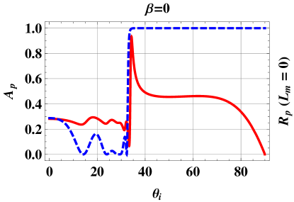
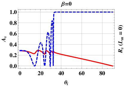
Figure 2: Left: Absorbance $A_{p}=1-(R_{pp}+R_{sp}+T_{pp}+T_{sp})$ (red, solid curve) plotted versus angle of incidence $\theta_{i}$ (in degree) for the case $\beta=0$; also plotted is the quantity $R_{p}=R_{pp}+R_{sp}$ (blue, dashed curve), calculated when $L_{m}=0$. Right: Absorbance $A_{s}=1-(R_{ss}+R_{ps}+T_{ss}+T_{ps})$ (red, solid curve) plotted versus angle of incidence $\theta_{i}$ (in degree) for the case $\beta=0$; also plotted is the quantity $R_{s}=R_{ss}+R_{ps}$ (blue, dashed curve), calculated when $L_{m}=0$.

Before considering the effects of relative motion, we must first establish the baseline for our studies, which is represented by the scenario wherein there is no relative motion. In Fig. 2, the absorbances $A_{p}$ and $A_{s}$ are plotted versus angle of incidence for the case $\beta=0$. Also plotted on these graphs are the quantities $R_{p}=R_{pp}+R_{sp}$ and $R_{s}=R_{ss}+R_{ps}$, calculated when the metal film is absent. A sharp high peak in the graph of $A_{p}$ at $\theta_{i}=34.2^{\circ}$ — which lies in the angular regime ${\cal R}_{p}$ for total reflection in the absence of the metal film — is the signature of SPP excitation by a $p$-polarized incident plane wave; for the chosen parameters, ${\cal R}_{p}=\left\{\theta_{i}|\theta_{i}>33.5^{\circ}\right\}$. This identification is further confirmed by the facts that (i) the $A_{p}$-peak remains at $\theta_{i}=34.2^{\circ}$ when the thickness of the dielectric slab is increased beyond 1000 nm and (ii) the eigenvalues of $\left[{\bf Q}(\epsilon^{\prime}_{d},\kappa^{\prime},\omega^{\prime})\right]$ evaluated at $\theta_{i}=34.2^{\circ}$ all have non–zero imaginary parts. There is no corresponding sharp high peak in the graph of $A_{s}$ in Fig. 2, in accordance with standard results [3, 4], although an angular regime ${\cal R}_{s}$ for total reflection in the absence of the metal film does exist; note that ${\cal R}_{p}\equiv{\cal R}_{s}$ when $\beta=0$.

3.1 Moving dielectric slab

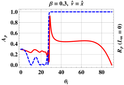
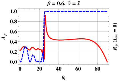
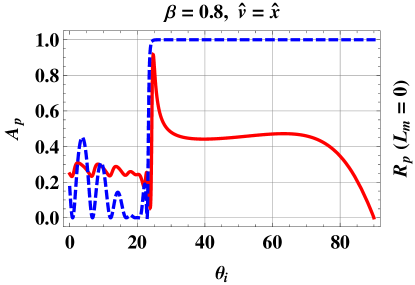
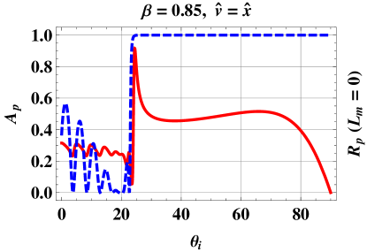
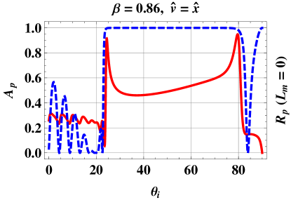
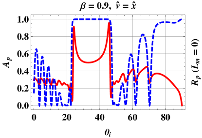
Figure 3: Absorbance $A_{p}=1-(R_{pp}+R_{sp}+T_{pp}+T_{sp})$ (red, solid curve) plotted versus angle of incidence $\theta_{i}$ (in degree) for the scenario where the dielectric slab moves in the direction $\hat{{\bf v}}=\hat{{\bf x}}$ at relative speeds $\beta\in\left\{0.3,0.6,0.8,0.85,0.86,0.9\right\}$. Also plotted is the quantity $R_{p}=R_{pp}+R_{sp}$ (blue, dashed curve), calculated when $L_{m}=0$.

Now we investigate the scenario schematically depicted in Fig. 1, where the dielectric slab moves at constant velocity parallel to the $x$ axis; i.e., $\hat{{\bf v}}=\hat{{\bf x}}$. The absorbance $A_{p}$ is plotted versus $\theta_{i}$ for the relative speeds $\beta\in\left\{0.3,0.6,0.8,0.85,0.86,0.9\right\}$ in Fig. 3. To confirm whether any possible SPP peaks occur in the angular regime ${\cal R}_{p}$, the quantity $R_{p}=R_{pp}+R_{sp}$, calculated when the metal film is absent, is also plotted.

The SPP peak in the plots of $A_{p}$ is found to arise at lower values of $\theta_{i}$ when $\beta$ increases from zero. Furthermore, the SPP peak in the plot of $A_{p}$ observed for $\beta\leq 0.85$ is joined by another prominent peak when $\beta>0.85$. For example, at $\beta=0.9$, there are prominent $A_{p}$-peaks at $\theta_{i}=\theta^{\sharp 1}_{i}=24.2^{\circ}$ and at $\theta_{i}=\theta^{\sharp 2}_{i}=45.7^{\circ}$. These values of $\theta^{\sharp 1}_{i}$ and $\theta^{\sharp 2}_{i}$ do not vary when the thickness of the dielectric slab is increased beyond 1000 nm; and all four eigenvalues of the matrix $\left[{\bf Q}(\epsilon^{\prime}_{d},\kappa^{\prime},\omega^{\prime})\right]$ evaluated at $\theta^{\sharp 1}_{i}$ and $\theta^{\sharp 2}_{i}$ have non–zero imaginary parts.

The plots of $R_{p}$ for $L_{m}=0$ in Fig. 3 indicate that the total reflection is not possible at $\beta>0.85$ for sufficiently large angles of incidence and therefore the significance of the two $A_{p}$-peaks at $\theta^{\sharp 1}_{i}$ and $\theta^{\sharp 2}_{i}$ is unclear. However, the $A_{p}$-peak at $\theta^{\sharp 1}_{i}$ corresponds to the SPP peak observed in the plots of $A_{p}$ for $\beta\leq 0.85$, as can be confirmed by tracking this peak while $\beta$ is continuously varied. The plots of $A_{s}$ (not shown here) corresponding to those of Fig. 3 for $\beta\in\left(0,1\right)$ do not exhibit SPP peaks.

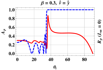
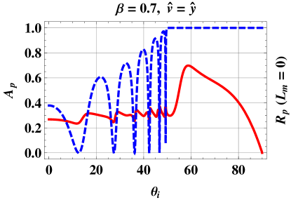
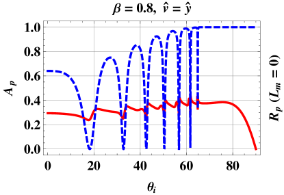
Figure 4: As Fig. 3 except that the dielectric slab moves in the direction $\hat{{\bf v}}=\hat{{\bf y}}$ and $\beta\in\left\{0.3,0.6,0.7,0.8\right\}$.

Next we consider the scenario where the dielectric slab moves at constant velocity parallel to the $y$ axis; i.e., $\hat{{\bf v}}=\hat{{\bf y}}$. The absorbance $A_{p}$, and the quantity $R_{p}$ calculated when the metal film is absent, are plotted versus $\theta_{i}$ for the relative speeds $\beta\in\left\{0.3,0.6,0.7,0.8\right\}$ in Fig. 4. Unlike for the case of $\hat{{\bf v}}=\hat{{\bf x}}$ in Fig. 3, now the value of $\theta_{i}$ at which the $A_{p}$-peak indicating the excitation of an SPP wave occurs increases as $\beta$ increases. Furthermore, this peak vanishes for $\beta\gtrsim 0.7$.

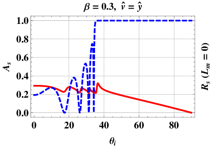
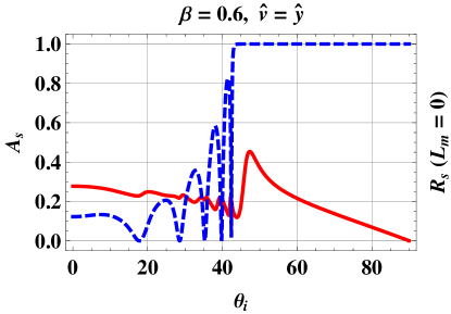
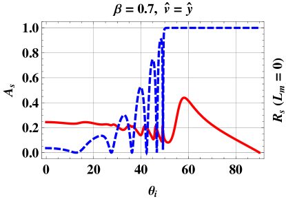
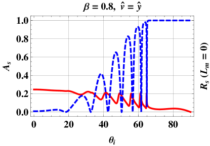
Figure 5: As Fig. 4 except that quantities plotted are $A_{s}=1-(R_{ss}+R_{ps}+T_{ss}+T_{ps})$ (red, solid curve) versus angle of incidence $\theta_{i}$ (in degree), and the quantity $R_{s}=R_{ss}+R_{ps}$ (blue, dashed curve), calculated when $L_{m}=0$.

The corresponding plots of absorbance for an $s$-polarized incident plane wave, provided in Fig. 5, exhibit a sharp peak for mid–range values of $\beta$, at angles of incidence in the angular regime ${\cal R}_{s}$. For example, this $A_{s}$-peak arises at $\theta_{i}=47.2^{\circ}$ for $\beta=0.6$. Further calculations have revealed that this peak is insensitive to changes in the thickness of the dielectric slab and all eigenvalues of $\left[{\bf Q}(\epsilon^{\prime}_{d},\kappa^{\prime},\omega^{\prime})\right]$ evaluated at $\theta_{i}=47.2^{\circ}$ have non–zero imaginary parts.

We therefore infer that, in the case of $\hat{{\bf v}}=\hat{{\bf y}}$, the SPP wave is excited by an incident $p$-polarized plane wave for low values of $\beta$, but excited by an incident $s$–polarized plane wave at higher values of $\beta$. As $\beta$ approaches unity, no absorbance peak indicating the excitation of an SPP wave is observed, for incident plane waves of either linear polarization state.

Clearly, from Figs. 3–5, the direction of motion has a major bearing on the excitation of SPP waves. This sensitivity to direction of motion reflects the fact that $\kappa\neq\kappa^{\prime}$ when motion is parallel to the plane of incidence but $\kappa=\kappa^{\prime}$ when motion is perpendicular to the plane of incidence, as may be inferred from (5).

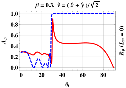
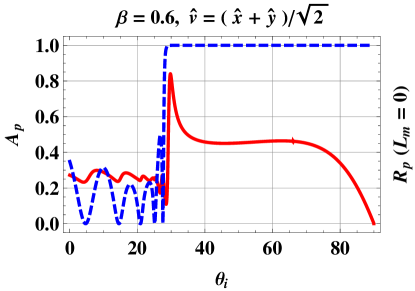
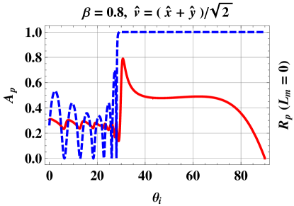
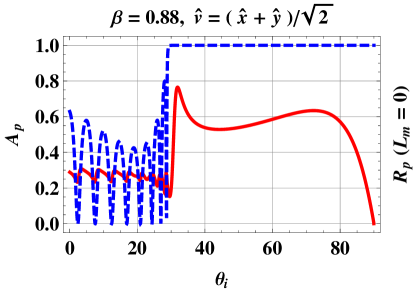
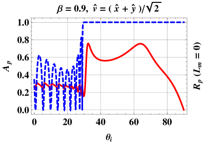
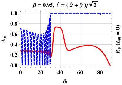
Figure 6: Absorbance $A_{p}=1-(R_{pp}+R_{sp}+T_{pp}+T_{sp})$ (red, solid curve) plotted versus angle of incidence $\theta_{i}$ (in degree) for the scenario where the dielectric slab moves in the direction $\hat{{\bf v}}=\left(\hat{{\bf x}}+\hat{{\bf y}}\right)/\sqrt{2}$ at relative speeds $\beta\in\left\{0.3,0.6,0.8,0.88,0.9,0.95\right\}$. Also plotted is the quantity $R_{p}=R_{pp}+R_{sp}$ (blue, dashed curve), calculated when $L_{m}=0$.

In order to further illuminate this issue, let us investigate the case where the direction of motion is neither parallel nor perpendicular to the plane of incidence; i.e., $\hat{{\bf v}}=\hat{{\bf x}}\cos\psi+\hat{{\bf y}}\sin\psi$ where, for example, we choose the angle $\psi=45^{\circ}$. In Fig. 6, the absorbance $A_{p}$, and the quantity $R_{p}$ calculated when the metal film is absent, are plotted versus $\theta_{i}$ for the relative speeds $\beta\in\left\{0.3,0.6,0.8,0.88,0.9,0.95\right\}$. The plots in Fig. 6 display some features of the plots presented in both Figs. 3 and 4. As is the case when motion is parallel to the plane of incidence, the solitary $A_{p}$-peak observed at low and moderate values of $\beta$ is joined by a second peak at higher values of $\beta$. A second $A_{p}$-peak begins to emerge in Fig. 6 at $\beta\approx 0.88$; it is fully developed at $\beta=0.9$; and as $\beta$ increases to approximately 0.95, the second $A_{p}$-peak coalesces with the first $A_{p}$-peak. For example, at $\beta=0.9$, there are $A_{p}$-peaks at $\theta_{i}=\theta^{\sharp 1}_{i}=32.3^{\circ}$ and at $\theta_{i}=\theta^{\sharp 2}_{i}=64.2^{\circ}$. The peak at $\theta^{\sharp 1}_{i}$ corresponds to the solitary SPP peak which is observed at low and moderate values of $\beta$. As is the case for the two high–$\beta$ $A_{p}$-peaks in Fig. 3, the values of $\theta^{\sharp 1}_{i}$ and $\theta^{\sharp 2}_{i}$ do not vary when the thickness of the dielectric slab is increased beyond 1000 nm; and all four eigenvalues of the matrix $\left[{\bf Q}(\epsilon^{\prime}_{d},\kappa^{\prime},\omega^{\prime})\right]$ evaluated at $\theta^{\sharp 1}_{i}$ and $\theta^{\sharp 2}_{i}$ have non–zero imaginary parts. We note that the $A_{p}$-peak at $\theta^{\sharp 1}_{i}$ is considerably sharper than the $A_{p}$-peak at $\theta^{\sharp 2}_{i}$.

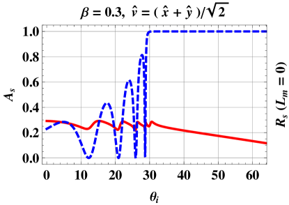
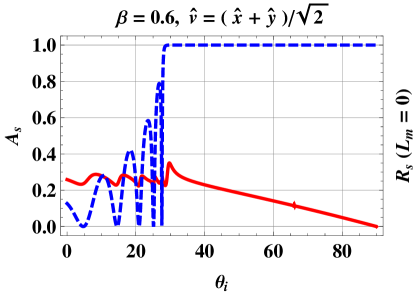
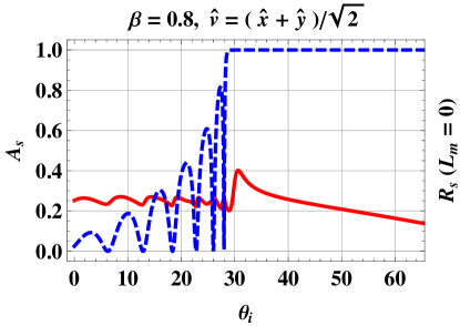
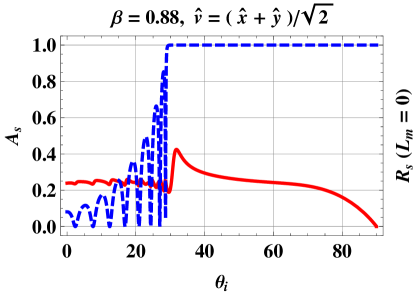
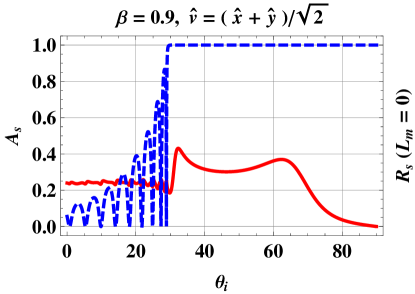
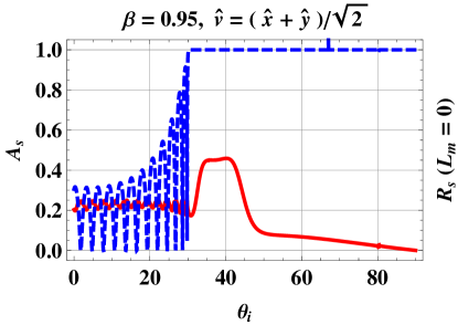
Figure 7: As Fig. 6 except that quantities plotted are $A_{s}=1-(R_{ss}+R_{ps}+T_{ss}+T_{ps})$ (red, solid curve) versus angle of incidence $\theta_{i}$ (in degree), and the quantity $R_{s}=R_{ss}+R_{ps}$ (blue, dashed curve), calculated when $L_{m}=0$.

The manifestation of an $A_{s}$-peak at moderate values of $\beta$, as may be observed in Fig. 5 when the motion is directed perpendicular to the plane of incidence, also occurs when motion is directed along $\hat{{\bf v}}=\left(\hat{{\bf x}}+\hat{{\bf y}}\right)/\sqrt{2}$, as is demonstrated by the plots presented in Fig. 7. Furthermore, the $A_{s}$ plots in Fig. 7 exhibit two $A_{s}$-peaks at high values of $\beta$, which coalesce as $\beta$ approaches unity, in a similar manner to the two $A_{p}$-peaks observed in Fig. 6.

3.2 Moving metal film

Next, we turn to a rather different situation. The dielectric slab is now held fixed relative to the half–spaces $z<0$ and $z>L_{\Sigma}$, whereas the metal film moves with velocity ${\bf v}=\beta c_{0}\hat{{\bf v}}$ in the $xy$ plane. The corresponding formulation is isomorphic to that presented in Sec. 2, but with the treatments for the metal film and the dielectric slab interchanged. For the case $\hat{{\bf v}}=\hat{{\bf x}}$, plots of $A_{p}$ versus $\theta_{i}$ (not shown here) are largely insensitive to $\beta$. That is, the $A_{p}$-peak indicating the excitation of an SPP wave occurs at approximately the same value of $\theta_{i}$ and has approximately the same amplitude, regardless of $\beta$. Furthermore, there are no notable peaks in the corresponding plots of $A_{s}$.

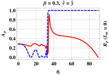
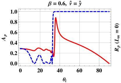
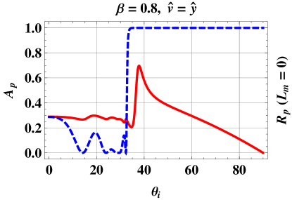
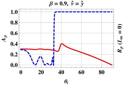
Figure 8: Absorbance $A_{p}=1-(R_{pp}+R_{sp}+T_{pp}+T_{sp})$ (red, solid curve) plotted versus angle of incidence $\theta_{i}$ (in degree) for the scenario where the metal film moves in the direction $\hat{{\bf v}}=\hat{{\bf y}}$ at relative speeds $\beta\in\left\{0.3,0.6,0.8,0.9\right\}$. Also plotted is the quantity $R_{p}=R_{pp}+R_{sp}$ (blue, dashed curve), calculated when $L_{m}=0$.

However, plots of $A_{p}$ in the case of $\hat{{\bf v}}=\hat{{\bf y}}$ are much more sensitive to $\beta$. As we can see in Fig. 8, the $A_{p}$-peak indicating the excitation of an SPP wave occurs at slightly higher values of $\theta_{i}$ as $\beta$ increases. Also, the amplitude of this peak gradually diminishes as $\beta$ increases, to such an extent that the peak is barely discernible at $\beta=0.9$. In the corresponding plots for a $s$–polarized incident plane wave (not shown here), there is a mere hint of an $A_{s}$-peak indicating the excitation of an SPP wave at mid–range values of $\beta$, but nothing as obvious as appears in the $s$-polarization scenario represented in Fig. 5.

4 Discussion

Uniform motion can have a major effect on the excitation of SPP waves guided by the interface of a metal film and a dielectric slab, both isotropic and homogeneous in their respective co-moving inertial reference frames. In the case of a uniformly moving dielectric slab, the angle of incidence for SPP-wave excitation is highly sensitive to the relative speed $\beta$ and the direction of motion. For the specific example considered in Sec. 3,

• when the direction of motion is parallel to the plane of incidence, the SPP wave is excited by $p$-polarized (but not $s$-polarized) incident plane waves for low and moderate values of $\beta$; and

• when the direction of motion is perpendicular to the plane of incidence, the SPP wave is excited by $p$-polarized incident plane waves for low values of $\beta$, but $s$-polarized incident plane waves at moderate values of $\beta$, while at higher values of $\beta$ the SPP wave is not excited.

Some insight into this sensitivity to relative motion can be gained by considering the Minkowski constitutive relations for the uniformly moving dielectric slab. That is, the electromagnetic response of the uniformly moving dielectric slab may be represented in the laboratory frame by the bianisotropic constitutive relations [19, Chap. 8]

$$\left.\begin{array}[]{l}\displaystyle{{\bf D}({\bf r},\omega)=\epsilon_{0}\epsilon^{\prime}_{d}\,\underline{\underline{\alpha}}\cdot{\bf E}({\bf r},\omega)+\frac{1}{c_{0}}\left({\bf m}\times\underline{\underline{I}}\,\right)\cdot{\bf H}({\bf r},\omega)\vspace{6pt}}\\ \displaystyle{{\bf B}({\bf r},\omega)=-\frac{1}{c_{0}}\left({\bf m}\times\underline{\underline{I}}\,\right)\cdot{\bf E}({\bf r},\omega)}+\mu_{0}\,\underline{\underline{\alpha}}\cdot{\bf H}({\bf r},\omega)\end{array}\right\},$$ (58)

where

$$\underline{\underline{\alpha}}=\alpha\,\underline{\underline{I}}+\left(1-\alpha\right)\,\hat{{\bf v}}\,\hat{{\bf v}},\qquad\alpha=\frac{1-\beta^{2}}{1-\epsilon^{\prime}_{d}\beta^{2}}$$ (59)

and

$${\bf m}=m\,\hat{{\bf v}},\qquad m=\frac{\beta\left(\epsilon^{\prime}_{d}-1\right)}{1-\epsilon^{\prime}_{d}\beta^{2}}.$$ (60)

Thus, when the direction of motion is parallel to the plane of incidence, for example, the Minkowski constitutive dyadics take the form

$$\left.\begin{array}[]{l}\underline{\underline{\alpha}}=\hat{{\bf x}}\,\hat{{\bf x}}+\alpha\left(\hat{{\bf y}}\,\hat{{\bf y}}+\hat{{\bf z}}\,\hat{{\bf z}}\right)\vspace{4pt}\\ {\bf m}\times\underline{\underline{I}}=m\left(\hat{{\bf z}}\,\hat{{\bf y}}-\hat{{\bf y}}\,\hat{{\bf z}}\right)\end{array}\right\}.$$ (61)

The Minkowski constitutive scalars $\alpha$ and $m$ for this case are plotted versus $\beta$ in Fig. 9. Clearly, the constitutive scalars are highly sensitive to $\beta$. Indeed, both $\alpha$ and $m$ become unbounded as $\beta\to 1/\sqrt{2}=0.707$. This singularity may be responsible for the break down of the total reflection regime and the anomalous second peak in the plots of $A_{p}$ and $A_{s}$ reported in Sec. 3 at high values of $\beta$.

In the case of a uniformly moving metal film, the sensitivity to $\beta$ is less obvious. Since the metal considered in Sec. 3 is dissipative — and quite highly, too — the Minkowski constitutive relations cannot be used here to gain an insight into the sensitivity to $\beta$ [18].

To conclude, our study further extends our understanding of electrodynamic processes at planar interfaces, especially relating to SPP waves.

Acknowledgments: TGM is supported by a Royal Academy of Engineering/Leverhulme Trust Senior Research Fellowship. AL thanks the Binder Endowment at Penn State for partial financial support of his research activities.

Figure 9: The Minkowski constitutive scalars $\alpha$ (red, solid curve) and $m$ (blue, dashed curve) of the dielectric slab plotted versus relative speed $\beta$ for the case where the direction of motion is parallel to the plane of incidence.

References

• [1] D. Felbacq, Plasmons go quantum, J. Nanophoton. 2 (2008) 020302.
• [2] J. Homola, Surface plasmon resonance sensors for detection of chemical and biological species, Chem. Rev. 108 (2008) 462–493, 2008.
• [3] I. Abdulhalim, M. Zourob, A. Lakhtakia, Surface plasmon resonance for biosensing: A mini-review, Electromagnetics 28 (2008) 214–242.
• [4] E. Kretschmann, H. Raether, Radiative decay of nonradiative surface plasmons excited by light, Z. Naturforsch. A 23 (1968) 2135–2136.
• [5] V.M. Agranovich, D.L. Mills (eds), Surface Polaritons: Electromagnetic Waves at Surfaces and Interfaces. North–Holland, Amsterdam, The Netherlands, 1982.
• [6] J.A. Polo Jr., A. Lakhtakia, Surface electromagnetic waves: A review, Laser & Photon. Rev., DOI: 10.1002/lpor.200900050 (2010).
• [7] G.J. Sprokel, The reflectivity of a liquid crystal cell in a surface plasmon experiment, Mol. Cryst. Liq. Cryst. 68 (1981) 39–45.
• [8] G.J. Sprokel, R. Santo, J.D. Swalen, Determination of the surface tilt angle by attenuated total reflection, Mol. Cryst. Liq. Cryst. 68 (1981) 29–38.
• [9] J.P. Lloyd, C. Pearson, M.C. Petty, Surface plasmon resonance studies of gas effects in phthalocyanine Langmuir–Blodgett films, Thin Solid Films 160 (1988) 431-443.
• [10] J. Singh, K. Thyagarajan, Analysis of metal clad uniaxial waveguides, Opt. Commun. 85 (1991) 397–402.
• [11] D. Mihalache, D.–M. Baboiu, M. Ciumac, L. Torner, J.P. Torres, Hybrid surface plasmon polaritons guided by ultrathin metal films, Opt. Quant. Electron. 26 (1994) 857–863.
• [12] H. Kano, W. Knoll, Locally excited surface-plasmon-polaritons for thickness measurement of LBK films, Opt. Commun. 153 (1998) 235–239.
• [13] J.A. Polo Jr., A. Lakhtakia, On the surface plasmon polariton wave at the planar interface of a metal and chiral sculptured thin film, Proc. R. Soc. A 465 (2009) 87–107.
• [14] M.A. Motyka, A. Lakhtakia, Multiple trains of same–color surface plasmon–polaritons guided by the planar interface of a metal and a sculptured nematic thin film, J. Nanophoton. 2 (2008) 021910.
• [15] M.A. Motyka, A. Lakhtakia, Multiple trains of same–color surface plasmon–polaritons guided by the planar interface of a metal and a sculptured nematic thin film. Part II: Arbitrary incidence, J. Nanophoton. 3 (2009) 033502.
• [16] A. Lakhtakia, Surface–plasmon wave at the planar interface of a metal film and a structurally chiral medium, Opt. Commun. 279 (2007) 291–297.
• [17] I.M. Besieris, R.T. Compton Jr.,Time-dependent Green’s function for electromagnetic waves in moving conducting media, J. Math. Phys. 8 (1967) 2445–2451.
• [18] T.G. Mackay, A. Lakhtakia, Positive-, negative-, and orthogonal-phase-velocity propagation of electromagnetic plane waves in a simply moving medium: Reformulation and reappraisal, Optik 120 (2009) 45–48.
• [19] H.C. Chen, Theory of Electromagnetic Waves, McGraw–Hill, New York, 1983.
• [20] T.G. Mackay, A. Lakhtakia, Electromagnetic Anisotropy and Bianisotropy: A Field Guide, Word Scientific, Singapore, 2010.
Refer to caption