Conductivity in the anisotropic background

Bum-Hoon Lee^a,b, Siyoung Nam^a, Da-Wei Pang^b and Chanyong Park^b

${}^{a}\,$Department of Physics, Sogang University, Seoul 121-742, Korea
${}^{b}\,$Center for Quantum Spacetime (CQUeST), Sogang University, Seoul 121-742, Korea

ABSTRACT

By using the gauge/gravity duality, we investigate the dual field theories of the anisotropic backgrounds, which are exact solutions of Einstein-Maxwell-dilaton theory with a Liouville potential. When we turn on the bulk gauge field fluctuation $A_{x}$ with a non-trivial dilaton coupling, the AC conductivity of this dual field theory is proportional to the frequency with an exponent depending on parameters of the anisotropic background. In some parameter regions, we find that this conductivity can have the negative exponent like the strange metal. In addition, we also investigate another $U(1)$ gauge field fluctuation, which is not coupled with a dilaton field. We classify all possible conductivities of this system and find that the exponent of the conductivity is always positive.

1 Introduction

The AdS/CFT correspondence[1, 2], which relates the dynamics of strongly coupled field theories to the corresponding dual gravity theories, has provided us a powerful tool for studying physical systems in the real world. Recently, inspired by condensed matter physics, the applications of the AdS/CFT correspondence to condensed matter physics(sometimes called the AdS/CMT correspondence) have been accelerated enormously. As a strong-weak duality, the AdS/CFT correspondence makes it possible to investigate the strongly coupled condensed matter systems in the dual gravity side. Therefore it is expected that we can acquire better understandings for certain condensed matter systems via the AdS/CFT correspondence. Some excellent reviews are given by [3].

According to the AdS/CFT correspondence, once the dual boundary field theory lies at finite temperature, there should exist a corresponding black hole solution in the bulk. Then some properties, like various conductivities [4, 5], superconductor [6, 7] and non-fermi liquid [8, 9], of the dual field theory can be inferred from the black hole. One particular class of such black hole solutions is a charged dilaton black hole [10, 11, 12, 13], where the gauge coupling of the Maxwell term is governed by a dilaton field $\phi$. Charged dilaton black holes in the presence of a Liouville potential were studied in Ref. [14]. Such charged dialton black hole solutions possess two interesting properties. First, for certain specific values of the gauge coupling, the charged dilaton black holes can be embedded into string theory. Second, the entropy vanishes in the extremal limit, which may signify that the thermodynamic description breaks down at extremality. Such peculiar features suggest that their AdS generalizations may provide interesting holographic descriptions of condensed matter systems.

Recently, holography of charged dilaton black holes in AdS₄ with planar symmetry was extensively investigated in [15]. The near horizon geometry was Lifshitz-like with a dynamical exponent $z$ determined by the dilaton coupling. The global solution was constructed via numerical methods and the attractor behavior was also discussed. The authors also examined the thermodynamics of near extremal black holes and computed the AC conductivity in zero-temperature background. For related works on charged dilaton black holes see [16, 17, 18, 19].

In this paper we focus on conductivities of charged dilaton black hole solutions [20] with a Liouville potential at both zero and finite temperature. At first we obtain exact solutions, both extremal and non-extremal, of the Einstein-Maxwell-dilaton theory, where the scalar potential takes the Liouville form. The extremal solution possesses anisotropic scaling symmetry which reduces to the Lifshitz-like metric [21] in a certain limit. In Ref. [15, 22], after inserting an irrelevant operator which deforms the asymptotic geometry to $AdS_{4}$, the electric conductivity was calculated. In this paper, we concentrate on the undeformed geometry and find exact solution describing undeformed geometry. Secondly we calculate the electric conductivity by considering the fluctuation of the gauge field $A_{x}$. The corresponding equation of motion for $A_{x}$ can be transformed into a Schrödinger equation, which enables us to evaluate the conductivity easily [6]. In the usual (deformed) AdS spaces, because there is no non-trivial dilaton coupling to the gauge field the conductivity of the dual theory is usually proportional to the frequency with the non-negative exponent, which is opposite to the strange metallic one. In the anisotropic background the electric conductivity generally is proportional to the frequency with an exponent determined by the non-trivial dilaton coupling and other background geometric parameters. Furthermore, in appropriate parameter regions we can find the strange metal-like conductivity proportional to the frequency with the negative exponent.

Next we introduce another $U(1)$ gauge field, which does not have a coupling with the dilaton field, and calculate the conductivity by considering the fluctuations of this new gauge field. There are some motivations for considering new gauge field with different dilaton coupling. First, if our four-dimensional gravity theory is originated from the ten dimensional string theory, there exist other many gauge fields having different dilaton coupling depending on how the string theory is compactified. Second, if we promote this bottom-up approach to the top-down approach, the gauge field living on the probe brane world volume typically has a dilaton coupling like $e^{-\phi}$. So studying the dynamics of the bulk gauge fluctuations having various dilaton couplings would shed light on understanding dual gauge theories. In this paper, we concentrate on a special case in which the gauge field fluctuation has no dilaton coupling and calculate the electric conductivities of the dual system. We find that the exponent of the conductivity for all parameter regions is always positive. This is the main difference between the dual theory with or without a non-trivial dilaton coupling, which implies that that the non-trivial dilaton coupling is very important to explain the strange metallic behavior.

The rest of the paper is organized as follows: in Section 2 we find the exact solutions of the charged dilaton black holes with a Liouville potential, both extremal and non-extremal. We calculate the conductivity by turning on the gauge field fluctuations coupled with the dilaton field in Section 3. In Section 4 we calculate the conductivity induced by a new $U(1)$ gauge field, which is not coupled with the dilaton field. Summary and discussion will be given in the final section.

Note added: In the final stage of this work, we noticed that similar solutions were studied extensively [22]. However, one key difference is that they required the solutions to be asymptotically $AdS$ while we treat the solutions to be global.

2 Anisotropic background with a Liouville potential

In the real condensed matter theory systems containing anisotropic scaling commonly appear. To describe this system holographically the Lifshitz background has been studied by many authors [21] by using the generalized AdS/CFT correspondence, so called the gauge/gravity duality. Here, we consider a different background having more general anisotropic scaling and investigate physical quantities of the dual field theory.

We start with the following action

$$S=\int d^{4}x\sqrt{-g}[R-2(\nabla\phi)^{2}-e^{2\alpha\phi}F_{\mu\nu}F^{\mu\nu}-V(\phi)],$$ (1)

where $\phi$ and $V(\phi)$ represent a dilaton field and its potential. Notice that the non-trivial dilaton coupling in front of the Maxwell term can provide a different physics from the ordinary relativistic field theory dual to AdS space. So main goal of the present work is to investigate the dilaton coupling effect on the physical quantity like the conductivity of the dual field theory. Equations of motion for metric $g_{\mu\nu}$, dilaton field and U(1) gauge field are

$$R_{\mu\nu}-\frac{1}{2}Rg_{\mu\nu}+\frac{1}{2}g_{\mu\nu}V(\phi) = 2\partial_{\mu}\phi\partial_{\nu}\phi-g_{\mu\nu}(\nabla\phi)^{2}+2e^{2\alpha\phi}F_{\mu\lambda}{F_{\nu}}^{\lambda}-\frac{1}{2}g_{\mu\nu}e^{2\alpha\phi}F^{2},$$ (2)

$$\partial_{\mu}(\sqrt{-g}\partial^{\mu}\phi) = \frac{1}{4}\sqrt{-g}\frac{\partial V(\phi)}{\partial\phi}+\frac{\alpha}{2}\sqrt{-g}e^{2\alpha\phi}F^{2},~{}~{}~{}$$ (3)

$$0 = \partial_{\mu}(\sqrt{-g}e^{2\alpha\phi}F^{\mu\nu}).$$ (4)

Now, we choose a Liouville-type potential as a dilaton potential

$$V(\phi)=2\Lambda e^{-\eta\phi}.$$ (5)

For $\eta=0$, the dilaton potential reduces to a cosmological constant, which was studied in Ref. [15]. To solve equations of motion, we use the following ansatz corresponding to a zero temperature solution

$$ds^{2}=-a(r)^{2}dt^{2}+\frac{dr^{2}}{a(r)^{2}}+b(r)^{2}(dx^{2}+dy^{2}),$$ (6)

with

$$a(r)=t_{0}r^{a_{1}},~{}~{}~{}b(r)=b_{0}r^{b_{1}},~{}~{}~{}\phi(r)=-k_{0}\log r.$$ (7)

If we turn on a time-component of the gauge field $A_{t}$ only, from the above metric ansatz the electric flux satisfying Eq. (4) becomes

$$F_{tr}=\frac{q}{b(r)^{2}}e^{-2\alpha\phi}.$$ (8)

The rest of equations of motion are satisfied when various parameters appearing in the above are given by

$$a_{1}=1+\frac{k_{0}}{2}\eta,~{}~{}~{}b_{1}=\frac{(2\alpha-\eta)^{2}}{(2\alpha-\eta)^{2}+16},~{}~{}~{}k_{0}=\frac{4(2\alpha-\eta)}{(2\alpha-\eta)^{2}+16},~{}~{}~{}b_{0}=1,$$

$$t_{0}^{2}=\frac{-2\Lambda}{(a_{1}+b_{1})(2a_{1}+2b_{1}-1)},~{}~{}~{}q^{2}=-\left(\frac{2k_{0}}{a_{1}+b_{1}}+\frac{\eta}{2}\right)\frac{\Lambda}{\alpha},$$ (9)

where $\Lambda$ is negative. This solution described by three free parameters $\alpha$, $\eta$ and $\Lambda$ is an exact solution of equations of motion. Notice that $b_{1}$ in Eq. (2) is always smaller than $1$. For $\eta=0$ and $\Lambda=-3$ this solution reduces to the one in Ref. [15], as previously mentioned. For $2\alpha=\eta$, the above solution becomes $AdS_{2}\times R^{2}$. If we take a limit $\alpha\to\infty$ and at the same time set $q=\eta=0$, we can obtain $AdS_{4}$ geometry. When $\eta$ is proportional to $\alpha$ like $\eta=c\alpha$, the metric in the limit, $\alpha\to\infty$, reduces to a Lifshitz-like one

$$ds^{2}=-t_{0}^{2}r^{2z}dt^{2}+\frac{dr^{2}}{t_{0}^{2}r^{2z}}+r^{2}\left(dx^{2}+dy^{2}\right),$$ (10)

with

$$z=\frac{2+c}{2-c}.$$ (11)

The exponent $z$ is given by $2$ for $c=2/3$ and $3$ for $c=1$, etc.

The above zero temperature solution can be easily extended to a finite temperature one describing a black hole. With the same parameters in Eq. (2), the black hole solution becomes

$$ds^{2}=-a(r)^{2}f(r)dt^{2}+\frac{dr^{2}}{a(r)^{2}f(r)}+b(r)^{2}(dx^{2}+dy^{2}),$$ (12)

where

$$f(r)=1-\frac{r^{2a_{1}+2b_{1}-1}_{h}}{r^{2a_{1}+2b_{1}-1}}.$$ (13)

Notice that since the above black hole factor does not include U(1) charge this solution corresponds to not a Reissner-Nordström but Schwarzschild black hole. The Hawking temperature of this black hole is given by

$$T\equiv\left.\frac{1}{4\pi}\frac{\partial(a(r)^{2}f)}{\partial r}\right|_{z=z_{h}}=\frac{(2a_{1}+2b_{1}-1)t_{0}^{2}r_{h}^{2a_{1}-1}}{4\pi},$$ (14)

where $r_{h}$ means the position of the black hole horizon.

3 Fluctuation of background gauge field $A_{x}$

In this section, we consider the gauge field fluctuation $A_{x}$ and calculate the electric conductivity of the dual theory. For convenience, we introduce new coordinate variable $u=r^{b_{1}}$. Then, the metric in Eq. (12) becomes

$$ds^{2}=-g(u)f(u)e^{-\chi(u)}dt^{2}+\frac{du^{2}}{g(u)f(u)}+u^{2}\left(dx^{2}+dy^{2}\right),$$ (15)

where

$$g(u) = t_{0}^{2}b_{1}^{2}u^{2(a_{1}+b_{1}-1)/b_{1}},$$

$$e^{\chi(u)} = b_{1}^{2}u^{2(b_{1}-1)/b_{1}},$$ (16)

with the black hole factor

$$f(u)=1-\frac{u_{h}^{(2a_{1}+2b_{1}-1)/b_{1}}}{u^{(2a_{1}+2b_{1}-1)/b_{1}}}.$$ (17)

On this background, we turn on the gauge field fluctuation $A_{x}$ together with the metric fluctuation $g_{tx}$. Although there is another relevant metric fluctuation $g_{ux}$, in the $g_{ux}=0$ and $A_{u}=0$ gauge only $A_{x}$ and $g_{tx}$ describe the vector fluctuations of the bulk theory. From the action for the gauge fluctuation

$$\delta S=-\frac{1}{4}\int d^{4}x\sqrt{-g}\ h^{2}F_{\mu\nu}F^{\mu\nu},$$ (18)

where $h^{2}=4e^{2\alpha\phi}$ is a coupling function, the equation of motion for $A_{x}$ becomes

$$0=\frac{1}{\sqrt{-g}}\partial_{\mu}\left(\sqrt{-g}\ h^{2}g^{\mu\rho}g^{x\nu}F_{\rho\nu}\right).$$ (19)

Under the following ansatz,

$$A_{x}(t,u) = \int\frac{dw}{2\pi}e^{-iwt}A_{x}(w,u),$$

$$g_{tx}(t,u) = \int\frac{dw}{2\pi}e^{-iwt}g_{tx}(w,u),$$ (20)

the above equation for $A_{x}$ can be rewritten as

$$0=\partial_{u}\left(e^{-\frac{\chi}{2}}gfh^{2}\partial_{u}A_{x}\right)+w^{2}e^{\frac{\chi}{2}}\frac{h^{2}}{gf}A_{x}+e^{\frac{\chi}{2}}h^{2}(\partial_{u}A_{t})\left(g_{tx}^{\prime}-\frac{2}{u}g_{tx}\right)$$ (21)

and the $(u,x)$-component of Einstein equation is given by

$$g_{tx}^{\prime}-\frac{2}{u}g_{tx}=-h^{2}(\partial_{u}A_{t})A_{x}.$$ (22)

Combining above two equations gives

$$0=\partial_{u}\left(e^{-\frac{\chi}{2}}gfh^{2}\partial_{u}A_{x}\right)+w^{2}e^{\frac{\chi}{2}}\frac{h^{2}}{gf}A_{x}-e^{\chi/2}h^{4}(\partial_{u}A_{t})^{2}A_{x}.$$ (23)

Introducing a new variable and new wave function

$$-\frac{\partial}{\partial v} = e^{-\frac{\chi}{2}}g\frac{\partial}{\partial u},$$

$$A_{x} = \frac{\Psi}{\sqrt{f}h},$$ (24)

Eq. (23) simply reduces to a Schrödinger-type equation

$$0=\Psi^{\prime\prime}+V(v)\Psi$$ (25)

with the effective potential

$$V(v)=\left(w^{2}+\frac{(f^{\prime})^{2}}{4}\right)\frac{1}{f^{2}}-\left(\frac{f^{\prime}h^{\prime}}{h}+\frac{f^{\prime\prime}}{2}+\frac{h^{2}}{g}e^{\chi}(A_{t}^{\prime})^{2}\right)\frac{1}{f}-\frac{h^{\prime\prime}}{h},$$ (26)

where the prime implies a derivative with respect to $v$. Using the first equation in Eq. (3) we can easily find $u$ as function of $v$. Here, we will concentrate on the case $2a_{1}>1$, in which $v$ is given by

$$v=\frac{1}{(2a_{1}-1)\ t_{0}^{2}\ u^{\frac{2a_{1}-1}{b_{1}}}}.$$ (27)

In $v$-coordinate the boundary ($u=\infty$) is located at $v=0$. In the black hole geometry, the black hole horizon $v_{h}$ is given by

$$v_{h}=\frac{1}{(2a_{1}-1)\ t_{0}^{2}\ u_{h}^{\frac{2a_{1}-1}{b_{1}}}}.$$ (28)

So the zero temperature corresponds to put the black hole horizon to $v=\infty$ ($u=0$).

3.1 At zero temperature

We first consider the zero temperature case, in which $f=1$ and $f^{\prime}=f^{\prime\prime}=0$. The effective potential Eq. (26) reduces to

$$V(v)=w^{2}-\frac{h^{2}}{g}e^{\chi}(A_{t}^{\prime})^{2}-\frac{h^{\prime\prime}}{h}.$$ (29)

Using Eq. (3), the above effective potential can be written as

$$V(v)=w^{2}-\frac{c}{v^{2}},$$ (30)

with a constant $c$

$$c=\frac{4(16+4\alpha^{2}-\eta^{2})\left[8+(2\alpha-\eta)(\alpha+\eta)\right]}{(16+4\alpha^{2}+4\alpha\eta-3\eta^{2})^{2}},$$ (31)

where we use Eq. (2). The exact solution $\Psi$ of the Schrödinger equation becomes

$$\Psi=c_{1}\sqrt{v}H^{(1)}_{\delta}(wv)+c_{2}\sqrt{v}H^{(2)}_{\delta}(wv),$$ (32)

where $H^{(i)}$ implies the $i$-th kind of Hankel function and

$$\delta=\frac{\sqrt{1+4c}}{2}.$$ (33)

At the horizon ($v=\infty$), the first or second term in Eq. (32) satisfies the incoming or outgoing boundary condition respectively. So to pick up the solution satisfying the incoming boundary condition we should set $c_{2}=0$. Then, the solution has the following expansion near the boundary

$$\Psi\approx\Psi_{0}\left(v^{\frac{1}{2}-\delta}-\left(\frac{w}{2}\right)^{2\delta}\frac{\Gamma(1-\delta)}{\Gamma(1+\delta)}e^{-i\pi\delta}v^{\frac{1}{2}+\delta}\right)$$ (34)

with

$$c_{1}=\frac{i\pi}{\Gamma(\delta)}\left(\frac{w}{2}\right)^{\delta}\Psi_{0}.$$ (35)

From this result together with Eq. (3), $A_{x}$ at the boundary ($u=\infty$) becomes

$$A_{x}=A_{0}\left(u^{\left[\alpha k_{0}-(2a_{1}-1)(\frac{1}{2}-\delta)\right]/b_{1}}-\tilde{c}\ u^{\left[\alpha k_{0}-(2a_{1}-1)(\frac{1}{2}+\delta)\right]/b_{1}}\right),$$ (36)

where

$$A_{0} = \frac{\Psi_{0}}{2\left[(2a_{1}-1)t_{0}^{2}\right]^{\frac{1}{2}-\delta}},$$

$$\tilde{c} = \left(\frac{w}{2}\right)^{2\delta}\frac{\Gamma(1-\delta)}{\Gamma(1+\delta)}\frac{e^{-i\pi\delta}}{\left[(2a_{1}-1)t_{0}^{2}\right]^{2\delta}}.$$ (37)

The boundary action for the gauge fluctuation $A_{x}$ becomes

$$S_{B} = -\frac{1}{2}\int d^{3}x\ \sqrt{-g}\ h^{2}g^{uu}g^{xx}A_{x}\ \partial_{u}A_{x}$$ (38)

$$= \frac{1}{2}\int d^{3}k\ 4t_{0}^{2}\tilde{c}\left[(2a_{1}-1)(\frac{1}{2}+\delta)-\alpha k_{0}\right]A_{0}^{2},$$

so that the Green function is given by

$$G_{xx}\equiv\frac{\partial^{2}S_{B}}{\partial A_{0}\partial A_{0}}=4t_{0}^{2}\left[(2a_{1}-1)(\frac{1}{2}+\delta)-\alpha k_{0}\right]\tilde{c}\sim w^{2\delta}.$$ (39)

Finally, the AC conductivity of the dual system reads off

$$\sigma=\frac{G_{xx}}{iw}\sim w^{2\delta-1}.$$ (40)

For the DC conductivity we should set $w=0$. Then, the DC conductivity of this system becomes infinity for $2\delta<1$ or zero for $2\delta>1$. In the real world, there exist some condensed matter systems having the AC conductivity with a negative exponent like the strange metal [23, 24]. If we choose $2\delta-1=-0.65$. the AC conductivity of this system can describes the strange metallic behavior $\sigma\sim w^{-0.65}$. Notice that since there are two free parameters, $\alpha$ and $\eta$, for $\Lambda=-3$ the strange metallic behavior can appear in infinitely many parameter regions. For example, the following parameters, $(\alpha,\eta)\approx(1,3.804),\ (2,5.196),\ (2,5.338),\cdots$, satisfy $\sigma\sim w^{-0.65}$ and give the regular value, $q^{2}>0$. As will be shown in Sec. 4, if we consider the gauge field fluctuation without the dilaton coupling the conductivity becomes a constant when the spatial momentum is zero. If turning on the spatial momentum, the conductivity always grows up as the frequency increases. These behaviors are different with those of the strange metal, which implies that the dilaton coupling of the gauge field plays an important role for describing the strange metallic behavior holographically. In the next section, we will show the strange metallic behavior at finite temperature.

3.2 At finite temperature

We consider the gauge and metric fluctuations at the finite temperature background. At the horizon, the dominant term in the effective potential in Eq. (26) is

$$U(v)\approx\left(w^{2}+\frac{(f_{h}^{\prime})^{2}}{4}\right)\frac{1}{f_{h}^{2}}=\left(w^{2}+\frac{(2a_{1}+2b_{1}-1)^{2}}{4(2a_{1}-1)^{2}v_{h}^{2}}\right)\frac{1}{f_{h}^{2}},$$ (41)

where $f_{h}$ means the value of $f$ at the horizon. Then, the approximate solution is given by

$$\Psi=c_{1}f^{\nu_{-}}+c_{2}f^{\nu_{+}},$$ (42)

where

$$\nu_{\pm}=\frac{1}{2}\pm i\sqrt{w^{2}+\frac{(2a_{1}+2b_{1}-1)^{2}}{4(2a_{1}-1)^{2}v_{h}^{2}}-\frac{1}{4}}.$$ (43)

Notice that at the horizon the first and second term in Eq. (42) satisfy the incoming and outgoing boundary condition respectively. Imposing the incoming boundary condition we can set $c_{2}=0$.

Now, we investigate the asymptotic behavior of $\Psi$. Since the leading behavior of the effective potential near the boundary is given by Eq. (30), the perturbative solution can be described by

$$\Psi=d_{1}\ v^{\frac{1}{2}-\delta}+d_{2}\ v^{\frac{1}{2}+\delta},$$ (44)

where $\delta$ has been defined in Eq. (33) together with Eq. (31). By solving Eq. (25) numerically, we can determine the numerical value of $d_{1}$ and $d_{2}$. In $u$-coordinate, the gauge field fluctuation has the following perturbative form

$$A_{x}=A_{0}\left(u^{\left[ak_{0}-(2a_{1}-1)(\frac{1}{2}-\delta)\right]/b_{1}}+\frac{d_{2}}{d_{1}\left[(2a_{1}-1)t_{0}^{2}\right]^{2\delta}}u^{\left[ak_{0}-(2a_{1}-1)(\frac{1}{2}+\delta)\right]/b_{1}}\right),$$ (45)

where to determine the boundary value of $A_{x}$ as $A_{0}$ we set

$$d_{1}=2\left[(2a_{1}-1)t_{0}^{2}\right]^{\frac{1}{2}-\delta}A_{0}.$$ (46)

The boundary action for $A_{x}$ becomes

$$S_{B}=\frac{A_{0}^{2}}{2}\int d^{3}x\ \frac{4t_{0}^{2}d_{2}\left[(2a_{1}-1)(\frac{1}{2}+\delta)+b_{1}-\alpha k_{0}\right]}{d_{1}\left[(2a_{1}-1)t_{0}^{2}\right]^{2\delta}}.$$ (47)

Then, we can easily find the AC conductivity at finite temperature

$$\sigma=\frac{4t_{0}^{2}}{iw}\left[(2a_{1}-1)(\frac{1}{2}+\delta)+b_{1}-\alpha k_{0}\right]\frac{d_{2}}{d_{1}\left[(2a_{1}-1)t_{0}^{2}\right]^{2\delta}},$$ (48)

where the last part $\frac{d_{2}}{d_{1}\left[(2a_{1}-1)t_{0}^{2}\right]^{2\delta}}$ can be numerically calculated by solving the Schrödinger equation together with the initial data at the horizon. In Figure 1, we plot the real and imaginary AC conductivity.

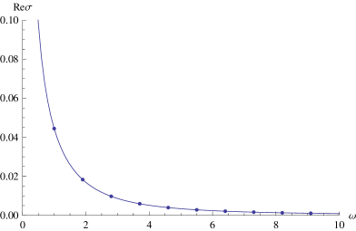
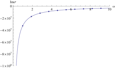
Figure 1: The conductivity at the finite temperature where we choose $\alpha=2$, $\eta=1$ and $\Lambda=-3$.

We can fit the dual AC conductivity of Figure 1 with the following expected form

$$\sigma=a\ w^{-b}.$$ (49)

If we choose $\alpha=2$, $\eta=1$ and $\Lambda=-3$ for the simple numerical calculation, the conductivity. can be fitted by Eq. (49) with $a\approx 0.045$ and $b\approx 1.5$.

4 New U(1) gauge field fluctuation

As mentioned in Introduction, it is interesting to investigate the conductivity of the gauge field having different dilaton coupling. Here, we will concentrate on new gauge field fluctuation having no dilaton coupling [25]. Even in this case, due to the parameters in the original action, we can find several different conductivities depending on the parameter region.

Before starting the calculation for the Green functions and conductivity in various parameter regions, we introduce a different coordinate $z=1/r$ for later convenience. In the $z$-coordinate, the black hole metric is rewritten as

$$ds^{2}=-\frac{t_{0}^{2}}{z^{2a_{1}}}f(z)dt^{2}+\frac{z^{2a_{1}}dz^{2}}{t_{0}^{2}z^{4}f(z)}+\frac{dx^{2}+dy^{2}}{z^{2b_{1}}}$$ (50)

with

$$f(z)=1-\frac{z^{2a_{1}+2b_{1}-1}}{z_{h}^{2a_{1}+2b_{1}-1}},$$ (51)

where all parameters are same as ones in Eq. (2) and $z_{h}$ implies the event horizon of the black hole. In this coordinate, the Hawking temperature becomes

$$T=\frac{(2a_{1}+2b_{1}-1)t_{0}^{2}}{4\pi z_{h}^{2a_{1}-1}}.$$ (52)

Now, we introduce another U(1) gauge field fluctuation, which is not coupled with a dilaton field

$$\delta S=-\frac{1}{4}\int d^{4}x\sqrt{-g}f_{\mu\nu}f^{\mu\nu},$$ (53)

where $f_{\mu\nu}=\partial_{\mu}a_{\nu}-\partial_{\nu}a_{\mu}$ and we absorb a gauge coupling constant to the gauge field. To obtain equations of motion for new gauge field, we first choose $a_{z}=0$ gauge and turn on the $x$-component of the gauge fluctuation only

$$a_{x}(x)=\int\frac{d^{3}k}{(2\pi)^{3}}e^{-iwt+i\vec{k}\cdot\vec{x}}a_{x}(k,z),$$ (54)

where a vector $\vec{x}$ corresponds to two-dimensional spatial coordinates. In the comoving frame, $\vec{k}=(w,0,k)$, the equation of this gauge fluctuation becomes

$$0=a_{x}^{\prime\prime}+\left(\frac{2(1-a_{1})}{z}+\frac{f^{\prime}}{f}\right)a_{x}^{\prime}+\left(\frac{w^{2}}{t_{0}^{4}z^{4(1-a_{1})}f^{2}}-\frac{k^{2}}{t_{0}^{2}z^{4-2a_{1}-2b_{1}}f}\right)a_{x},$$ (55)

where the prime implies a derivative with respect to $z$ and $f$ is a black hole factor.

4.1 At zero temperature

In this section, we investigate various Green functions at zero temperature, which can be obtained by setting $f=1$ and $f^{\prime}=0$.

4.1.1 for $a_{1}\leq 1$

Notice that $b_{1}$, as mentioned previously, is always smaller than $1$ and the case, $b_{1}=1$, can be considered as the limit $\alpha\to\infty$.

i) $\frac{1}{2}<a_{1}=b_{1}\leq 1$

At first, we consider a simple case $a_{1}=b_{1}\leq 1$. In this case, the equation governing the transverse gauge field fluctuation becomes

$$0 = a_{x}^{\prime\prime}+\frac{2\delta}{z}a_{x}^{\prime}+\frac{\gamma}{z^{4\delta}}a_{x},$$ (56)

with

$$\delta=1-a_{1}\qquad{\rm and}\qquad\gamma=\frac{w^{2}}{t_{0}^{4}}-\frac{k^{2}}{t_{0}^{2}},$$ (57)

where $0\leq\delta<1$. The exact solution of the above equation is given by

$$a_{x}=c_{1}\exp(i\frac{\sqrt{\gamma}z^{1-2\delta}}{1-2\delta})+c_{2}\exp(-i\frac{\sqrt{\gamma}z^{1-2\delta}}{1-2\delta}).$$ (58)

At the horizon ($z\to\infty$), the first or second term satisfies the incoming or outgoing boundary condition respectively. Imposing the incoming boundary condition, the solution reduces to

$$a_{x}=c_{1}\exp\left(i\frac{\sqrt{\gamma}}{1-2\delta}z^{1-2\delta}\right).$$ (59)

For $\delta>1/2$, we can not purturbatively expand this solution near the boundary ($z=0$). In such case it is unclear how to define the dual operator, so we consider only the case $\delta<1/2$ (or $a_{1}>1/2$) from now on. In this case, $a_{x}$ has the following expansion near the boundary

$$a_{x}=a_{0}\left(1+i\frac{\sqrt{\gamma}}{1-2\delta}z^{1-2\delta}+\cdots\right),$$ (60)

where $a_{0}=c_{1}$ corresponds to the boundary value of $a_{x}$, which can be identified with the source term of the dual gauge operator. According to the gauge/gravity duality, the on-shell gravity action can be interpreted as a generating functional for the dual gauge operator. The on-shell gravity action corresponding to the boundary action is given by

$$S_{B}=\frac{1}{2}\int d^{3}x\ \sqrt{-g}\ g^{zz}g^{xx}a_{x}\ \partial_{z}a_{x}=\frac{ia_{0}^{2}}{2}\int d^{3}kt_{0}^{2}\sqrt{\gamma}.$$ (61)

Using this on-shell action we can easily calculate the Green function by varying the on-shell action with respect to the source.

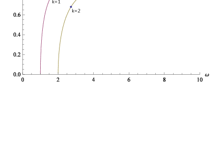
Figure 2: The real and imaginary conductivity at $t_{0}=1$ with $a_{1}=b_{1}\leq 1$.

For $a_{x}$, the Green function becomes

$$G_{xx}\equiv\frac{\partial^{2}S_{B}}{\partial a_{0}\partial a_{0}}=iw\sqrt{1-\frac{k^{2}t_{0}^{2}}{w^{2}}},$$ (62)

and the conductivity of the dual system is given by

$$\sigma=\frac{G_{xx}}{iw}=\sqrt{1-\frac{t_{0}^{2}k^{2}}{w^{2}}}.$$ (63)

For the time-like case ($w^{2}>k^{2}t_{0}^{2}$), the conductivity is real. In the space-like case, the imaginary conductivity appears. In addition, the AC conductivity for $k=0$ becomes a constant $\sigma_{AC}=1$, in which there is no imaginary part of the conductivity. In Figure 2, we plot the real and imaginary conductivity, in which we can see that as the momentum $k$ increases the real or imaginary conductivity decreases or increases respectively. Furthermore, as shown in Eq. (63) and figure 2, the real and imaginary conductivities become zero at $w^{2}=t_{0}^{2}k^{2}$. Below or above this critical point, there exists only the imaginary or real conductivity respectively.

ii) $\frac{1}{2}<b_{1}<a_{1}\leq 1$

It is impossible to solve Eq. (55) analytically with arbitrary parameters $a_{1}$ and $b_{1}$. So, instead of solving Eq. (55) analytically, we will try to find a Green function and electric conductivity numerically. To do so, we should first know the perturbative behavior of $a_{x}$ near the horizon as well as the asymptotic boundary.

At the horizon, since $1/z^{4(1-a_{1})}$ term in Eq. (55) is dominant, the approximate solution satisfying the incoming boundary condition is given by

$$a_{x}=c\exp\left(i\frac{w}{t_{0}^{2}(2a_{1}-1)}z^{2a_{1}-1}\right).$$ (64)

Near the boundary, $1/z^{4-2a_{1}-2b_{1}}$ term in Eq. (55) is dominant, so Eq. (55) is reduced to

$$0=a_{x}^{\prime\prime}+\frac{2(1-a_{1})}{z}a_{x}^{\prime}-\frac{k^{2}}{t_{0}^{2}z^{4-2a_{1}-2b_{1}}}a_{x}.$$ (65)

The leading two terms of asymptotic solution are

$$a_{x}=c_{1}+c_{2}z^{2a_{1}-1},$$ (66)

where $c_{1}$ and $c_{2}$ are integration constants. To find a relation between two integration constants and $c$, we should solve Eq. (55) numerically with the initial conditions determined from Eq. (64). To control the limit $z\to\infty$ we introduce an IR cut-off $z_{0}$, which is a very large number. At this IR cut-off, $a_{x}$ and $a_{x}^{\prime}$ become

$$a_{x}(z_{0}) = c\exp\left(i\frac{w}{t_{0}^{2}(2a_{1}-1)}z_{0}^{2a_{1}-1}\right),$$

$$a_{x}^{\prime}(z_{0}) = \frac{icw\ z_{0}^{2a_{1}-2}}{t_{0}^{2}}\exp\left(i\frac{w}{t_{0}^{2}(2a_{1}-1)}z_{0}^{2a_{1}-1}\right).$$ (67)

Using these initial values, we can solve Eq. (55) numerically and find numerical values for $a_{x}(\epsilon)$ and $a_{x}^{\prime}(\epsilon)$, where $\epsilon$($\epsilon\to 0$) means an UV cut-off. Then, two integration constants $c_{1}$ and $c_{2}$ can be determined by $a_{x}(\epsilon)$ and $a_{x}^{\prime}(\epsilon)$

$$c_{1} = a_{x}(\epsilon),$$

$$c_{2} = \frac{a_{x}^{\prime}(\epsilon)}{(2a_{1}-1)\epsilon^{2a_{1}-2}}.$$ (68)

If we identify the boundary value of $a_{x}$ with a source term $a_{0}$

$$a_{0}=\lim_{\epsilon\to 0}a_{x}(\epsilon).$$ (69)

$c_{1}$ and $c_{2}$ correspond to a source and the expectation value of the boundary dual operator respectively. Then, from the boundary action the electric conductivity becomes

$$\sigma=\frac{t_{0}^{2}a_{x}^{\prime}(\epsilon)}{iwa_{x}(\epsilon)\epsilon^{2a_{1}-2}}.$$ (70)

In Figure 3, we plot the real and imaginary conductivity. Notice that in this case there is no critical point like the $\frac{1}{2}<a_{1}=b_{1}\leq 1$ case. In other words, the real and imaginary conductivity is well defined on the whole range of the frequency. Especially, for large $k$ the real conductivity becomes zero as the frequency goes to zero. For $k=0$, the real conductivity is a constant like the previous case. For $k\neq 0$ the conductivity grows as the frequency increases, which is opposite to the strange metallic conductivity.

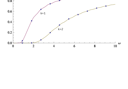
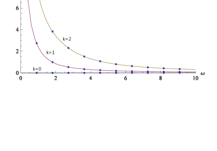
Figure 3: The real and imaginary conductivity at $t_{0}=1$ with $\frac{1}{2}<b_{1}<a_{1}\leq 1$.

iii) $\frac{1}{2}<a_{1}<b_{1}\leq 1$

In this case, $k^{2}$ term in Eq. (55) is dominant at the horizon. Due to the sign of it, the near horizon behavior of this solution is space-like. So we should impose the regularity condition instead of the incoming boundary condition. More precisely, in this parameter region the equation governing $a_{x}$ at the horizon reduces to Eq. (65). The exact solution of it is given by

$$a_{x}=z^{a_{1}-\frac{1}{2}}\left(d_{1}^{\prime}I_{-\nu}\left(x\right)+d_{2}^{\prime}I_{\nu}\left(x\right)\right),$$ (71)

with two integration constants $d_{1}^{\prime}$ and $d_{2}^{\prime}$, where $I_{\nu}(x)$ is a modified Bessel function and

$$\nu=\frac{2a_{1}-1}{2(a_{1}+b_{1}-1)}\qquad{\rm and}\qquad x=\frac{kz^{a_{1}+b_{1}-1}}{t_{0}(a_{1}+b_{1}-1)}.$$ (72)

At the horizon, the leading terms of it become

$$a_{x}=\frac{1}{z^{(b_{1}-a_{1})/2}}\left[d_{1}\exp\left(-\frac{kz^{a_{1}+b_{1}-1}}{t_{0}(a_{1}+b_{1}-1)}\right)+d_{2}\exp\left(\frac{kz^{a_{1}+b_{1}-1}}{t_{0}(a_{1}+b_{1}-1)}\right)\right],$$ (73)

where $d_{1}$ and $d_{2}$ are different constants with $d_{1}^{\prime}$ and $d_{2}^{\prime}$. In the above, the second term diverges at the horizon $z\to\infty$, so we can pick up the regular solution by imposing the regularity at the horizon, which is the same as imposing the incoming boundary condition when $k\to-ik$. From the horizon solution

$$a_{x}=\frac{d_{1}\exp\left(-\frac{kz^{a_{1}+b_{1}-1}}{t_{0}(a_{1}+b_{1}-1)}\right)}{z^{(b_{1}-a_{1})/2}},$$ (74)

we can determine initial values for $a_{x}(z_{0})$ and $a_{x}^{\prime}(z_{0})$ at the IR cut-off $z_{0}$. The near boundary solution in $\frac{1}{2}<a_{1}<b_{1}\leq 1$ is also given by the same form in Eq. (66).

Before calculating the Green function and electric conductivity, notice that $a_{x}$ in Eq. (74) is real due to the regularity condition at the horizon. So the resulting Green function is also real, which implies that the conductivity is a pure imaginary number. Following the technique explained in the previous section, the unknown integration constants $c_{1}$ and $c_{2}$ can be determined by the boundary values $a_{x}(\epsilon)$ and $a_{x}^{\prime}(\epsilon)$ after solving Eq. (55) numerically. Figure 4 shows the imaginary conductivity.

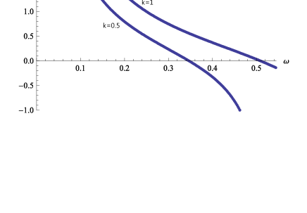
Figure 4: The imaginary conductivity at $t_{0}=1$ with $\frac{1}{2}<a_{1}<b_{1}\leq 1$.

4.1.2 for $a_{1}>1$

In this case, the equation for $a_{x}$ becomes

$$0=a_{x}^{\prime\prime}-\frac{2(a_{1}-1)}{z}a_{x}^{\prime}+\left(\frac{w^{2}}{t_{0}^{4}}z^{4(a_{1}-1)}-\frac{k^{2}}{t_{0}^{2}}z^{2(a_{1}+b_{1}-2)}\right)a_{x}.$$ (75)

At the horizon($z\to\infty$), the first term proportional to $w^{2}$ is dominant, so the approximate solution satisfying the incoming boundary condition is given by

$$a_{x}\approx\ \exp\left(\frac{iwz^{2a_{1}-1}}{t_{0}^{2}(2a_{1}-1)}\right).$$ (76)

For $k=0$, the above is an exact solution satisfying the incoming boundary condition, which is the same as one in Eq. (59) with $k=0$. In this case, from the result in Eq. (63) we can easily find that the conductivity becomes $1$. Notice that in Figure 5 the numerical calculation for the conductivity at $k=0$ gives the same result obtained by analytic calculation.

Near the boundary ($z\to 0$), the $k^{2}$ term is dominant, so the approximate solution becomes

$$a_{x}\approx a_{0}\left(1+c\ z^{2a_{1}-1}\right),$$ (77)

where $a_{0}$ is the boundary value of $a_{x}$. To determine a constant $c$, we numerically solve the differential equation in Eq. (75) with the initial values given at the horizon. Then, we can find the values for $a_{x}$ and $a_{x}^{\prime}$ at the boundary. Comparing these results with Eq. (77), we can determine the unknown constant $c$ numerically. Using these results, the Green functions and conductivity are given by

$$G_{xx} = t_{0}^{2}(2a_{1}-1)c,$$

$$\sigma = \frac{G_{xx}}{iw}.$$ (78)

In Figure 5, we present several conductivity plots depending on the momentum, which is very similar to one obtained in the $\frac{1}{2}<b_{1}<a_{1}\leq 1$ case. Notice that for $\frac{1}{2}<b_{1}<a_{1}\leq 1$ and $a_{1}>1$ the DC conductivity is zero for $k=1$ or $2$.

4.2 At finite temperature

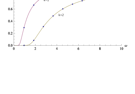
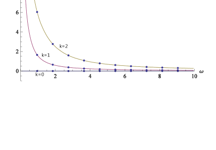
Figure 5: The real and imaginary conductivity when $a_{1}=5/4$, $b_{1}=3/4$ and $t_{0}=1$ .

First, we consider the simplest case $k=0$ in which we can obtain an exact solution. To solve Eq. (55), we introduce a new coordinate

$$du=\frac{dz}{z^{2-2a_{1}}f}.$$ (79)

Then, in the $u$-coordinate Eq. (55) for $k=0$ reduces to

$$0=\partial_{u}^{2}a_{x}+\frac{w^{2}}{t_{0}^{4}}a_{x},$$ (80)

where the relation between $u$ and $z$ is given by

$$u=\frac{z^{2a_{1}-1}}{2a_{1}-1}\ _{2}F_{1}\left(\frac{2a_{1}-1}{2a_{1}+2b_{1}-1},\frac{2(2a_{1}+b_{1}-1)}{2a_{1}+2b_{1}-1},z^{2a_{1}+2b_{1}-1}\right).$$ (81)

Near the horizon ($z\sim z_{h}$), the above relation becomes

$$u\approx-\frac{z_{h}^{2a_{1}-1}}{2a_{1}+2b_{1}-1}\log(z_{h}-z),$$ (82)

so the horizon lies at $u=\infty$ for $a_{1}>1/2$. Near the boundary ($z\to 0$), $u$ is related to $z$

$$u\approx\frac{z^{2a_{1}-1}}{2a_{1}-1}.$$ (83)

At the horizon, the solution of Eq. (80) satisfying the incoming boundary condition is given by

$$a_{x}=a_{0}\exp\left(i\frac{wu}{t_{0}^{2}}\right),$$ (84)

where $a_{0}$ is the boundary value of $a_{x}$. Near the boundary, the expansion of the above solution becomes

$$a_{x}=a_{0}\left(1+i\frac{w}{(2a_{1}-1)t_{0}^{2}}z^{2a_{1}-1}\right),$$ (85)

which is the same as one in the zero temperature case. Therefore, the Green function and conductivity for $k=0$ is the same as the zero temperature result.

Now, we consider the general case with non-zero $k$. In this case, it is very difficult to find an analytic solution, so we adopt a numerical method. Since the black hole factor $f$ becomes zero at the horizon ($z\to z_{h}$), the differential equation in Eq. (55) near the horizon reduces to

$$0=a_{x}^{\prime\prime}+\frac{f^{\prime}}{f}a_{x}^{\prime}+\frac{w^{2}}{t_{0}^{4}z^{4(1-a_{1})}f^{2}}a_{x},$$ (86)

where

$$f=1-\frac{z^{2a_{1}+2b_{1}-1}}{z_{h}^{2a_{1}+2b_{1}-1}}.$$ (87)

The leading term of the solution satisfying the incoming boundary condition is

$$a_{x}=cf^{-i\nu}\left(1+\cdots\right),$$ (88)

with

$$\nu=\frac{w\ z_{h}^{2a_{1}-1}}{{(2a_{1}+2b_{1}-1)\ t_{0}^{2}}},$$ (89)

where the ellipsis implies higher order terms and $c$ is an integration constant. Since at $z=z_{h}$ $a_{x}$ and $a_{x}^{\prime}$ become zero, we pick up the initial values at $z_{i}=z_{h}-\epsilon$, where $\epsilon$ is a very small number, for solving the differential equation numerically. After solving Eq. (55), we can find numerical values for $a_{x}(\epsilon)$ and $a_{x}^{\prime}(\epsilon)$, where $\epsilon$ is a small number, up to multiplication constant $c$ at the boundary.

To understand the boundary behavior of $a_{x}$, we should know the perturbative form of $a_{x}$ near the boundary. From Eq. (55), the perturbative solution near the boundary is given by

$$a_{x}=a_{0}\left(1+A\ z^{2a_{1}-1}\right),$$ (90)

where $a_{0}$ is the boundary value of $a_{x}$ and $A$ is an integration constant, which will be determined later. Using the above numerical results $a_{x}(\epsilon)$ and $a_{x}^{\prime}(\epsilon)$, $a_{x}$ can be written as

$$a_{x}(z)=c\left(a_{x}(\epsilon)+\frac{a_{x}^{\prime}(\epsilon)}{2a_{1}-1}\ \frac{z^{2a_{1}-1}}{\epsilon^{2a_{1}-2}}\right),$$ (91)

Matching this value with Eq. (90) gives $c=\frac{a_{0}}{a_{x}(\epsilon)}$ and $A$ becomes

$$A=\frac{a_{x}^{\prime}(\epsilon)}{(2a_{1}-1)\epsilon^{2a_{1}-2}a_{x}(\epsilon)}.$$ (92)

Therefore, the Green function and conductivity can be written as

$$G_{xx} = (2a_{1}-1)t_{0}^{2}A,$$

$$\sigma \equiv \frac{G_{xx}}{iw}=\frac{t_{0}^{2}}{iw\epsilon^{2a_{1}-2}}\frac{a_{x}^{\prime}(\epsilon)}{a_{x}(\epsilon)}.$$ (93)

Figure 6 shows the conductivity at finite temperature. Similarly to the zero temperature cases, for $k=0$ the real conductivity is still a constant. But for $k=1$ or $2$, the finite temperature conductivity goes to a constant as the frequency goes to zero, while the zero temperature one approaches to zero. This implies that the finite temperature DC conductivity is a constant while the zero temperature DC conductivity is zero. We can also see that like the zero temperature case the conductivity grows as the frequency increases, which is different with the strange metallic behavior. Moreover, since our background geometry is not a maximally symmetric space, the dual boundary theory is not conformal. So we can expect that there exists the non-trivial temperature dependence of the conductivity. In Figure 7 we plot the electric conductivity depending on temperature.

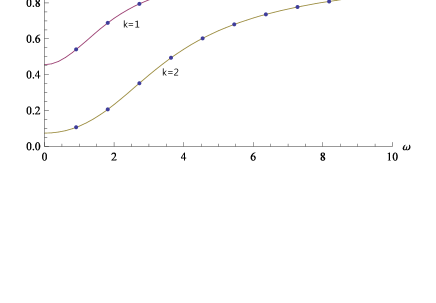
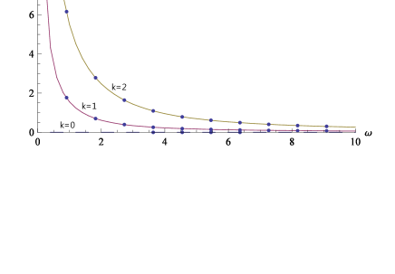
Figure 6: The real and imaginary conductivity at finite temperature $T=0.239$ ($z_{h}=1$) when $a_{1}=5/4$, $b_{1}=3/4$ and $t_{0}=1$ .

5 Discussion

There exist two complementary approaches for studying applications of the gauge/gravity duality to condensed matter systems. One is the bottom-up approach in which on a given gravity solution we investigate the dual field theory. The other is the top-down approach in which, after considering the probe brane configuration on the geometry obtained from the string theory, the dual field theory is investigated by studying various fluctuations on the probe brane. In this paper we mainly adopt the bottom-up approach. For the top-down approach, see Ref. [26].

Due to the peculiar properties, charged dilaton black holes may provide new backgrounds for describing the gravity duals of certain condensed matter systems. In this paper we studied conductivities of charged dilaton black holes with a Liouville potential both at zero and finite temperature. In general, the anisotropic (charged dilaton) black hole has three free parameters. Depending on which parameters we choose, the anisotropic background can reduce to $AdS_{4}$, $AdS_{2}\times S^{2}$ and the Lifshitz-like space. To investigate the dual theory which may describe some aspects of the condensed matter system, we have calculated its electric conductivity in various parameter regions.

First, we have considered the gauge fluctuation of the background gauge field, which is coupled with the dilaton field. Due to this non-trivial dilaton coupling, the conductivity of this system depends on the frequency non-trivially. After choosing appropriate parameters, at both zero and finite temperature we obtained the strange metal-like AC conductivity proportional to the frequency with a negative exponent. Because our model have three free parameters, it may shed light on investigating other dual field theory having more general exponent.

Second, we have also investigated another dual field theory whose dual gravity theory has the another U(1) gauge field fluctuation without the dilaton coupling. Due to the parameters in the original action, there are several parameter regions giving different conductivities. We have classified all possible conductivities either analytically or numerically. Here, we found that the conductivities for $k=0$ at zero and finite temperature become a constant because there is no dilaton coupling with the new gauge field fluctuation. This implies that to describe the non-trivial conductivity depending on the frequency like the strange metal, it would be important to consider the dilaton coupling effect at least in the bottom-up approach. We have also investigated the conductivity depending on the spatial momentum and the temperature. As the spatial momentum increases we found that the real conductivity goes down. In addition, we found that the finite temperature DC conductivity becomes a non-zero constant while the zero temperature one is zero in this set-up.

One further generalization is to incorporate the magnetic field and to find dyonic black hole solutions. Once we find such exact solutions carrying both electric and magnetic charges, it would be interesting to study the thermodynamics and transport coefficients, such as the Hall conductivity [5], in the presence of the magnetic field. Another interesting direction is to study the non-Fermi liquid behavior in the solutions we obtained, following [8, 9, 27, 28]. We hope to report some results about such fascinating topics in the future.

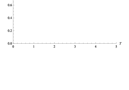
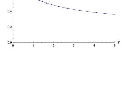
Figure 7: The real and imaginary conductivity depending on temperature when $w=2$, $k=1$, $a_{1}=5/4$, $b_{1}=3/4$ and $t_{0}=1$ .

Acknowledgements

This work was supported by the National Research Foundation of Korea (NRF) grant funded by the Korea government (MEST) through the Center for Quantum Spacetime (CQUeST) of Sogang University with grant number 2005-0049409. C. Park was also supported by Basic Science Research Program through the National Research Foundation of Korea(NRF) funded by the Ministry of Education, Science and Technology(2010-0022369).

References

- [1] J. M. Maldacena, “The large N limit of superconformal field theories and supergravity,” Adv. Theor. Math. Phys. 2, 231 (1998) [Int. J. Theor. Phys. 38, 1113 (1999)] [arXiv:hep-th/9711200]; S. S. Gubser, I. R. Klebanov and A. M. Polyakov, “Gauge theory correlators from non-critical string theory,” Phys. Lett. B 428, 105 (1998) [arXiv:hep-th/9802109]; E. Witten, “Anti-de Sitter space and holography,” Adv. Theor. Math. Phys. 2, 253 (1998) [arXiv:hep-th/9802150].
- [2] O. Aharony, S. S. Gubser, J. M. Maldacena, H. Ooguri and Y. Oz, “Large N field theories, string theory and gravity,” Phys. Rept. 323, 183 (2000) [arXiv:hep-th/9905111].
- [3] S. A. Hartnoll, “Lectures on holographic methods for condensed matter physics,” Class. Quant. Grav. 26, 224002 (2009) [arXiv:0903.3246 [hep-th]]; C. P. Herzog, “Lectures on Holographic Superfluidity and Superconductivity,” J. Phys. A 42, 343001 (2009) [arXiv:0904.1975 [hep-th]]; J. McGreevy, “Holographic duality with a view toward many-body physics,” arXiv:0909.0518 [hep-th]; G. T. Horowitz, “Introduction to Holographic Superconductors,” arXiv:1002.1722 [hep-th]; S. Sachdev, “Condensed matter and AdS/CFT,” arXiv:1002.2947 [hep-th].
- [4] S. S. Gubser and F. D. Rocha, “The gravity dual to a quantum critical point with spontaneous symmetry breaking,” Phys. Rev. Lett. 102, 061601 (2009) [arXiv:0807.1737 [hep-th]].
- [5] S. A. Hartnoll and P. Kovtun, “Hall conductivity from dyonic black holes,” Phys. Rev. D 76, 066001 (2007) [arXiv:0704.1160 [hep-th]].
- [6] G. T. Horowitz and M. M. Roberts, “Zero Temperature Limit of Holographic Superconductors,” JHEP 0911, 015 (2009) [arXiv:0908.3677 [hep-th]].
- [7] S. A. Hartnoll, C. P. Herzog and G. T. Horowitz, “Holographic Superconductors,” JHEP 0812, 015 (2008) [arXiv:0810.1563 [hep-th]].
- [8] S. S. Lee, “A Non-Fermi Liquid from a Charged Black Hole: A Critical Fermi Ball,” Phys. Rev. D 79, 086006 (2009) [arXiv:0809.3402 [hep-th]].
- [9] H. Liu, J. McGreevy and D. Vegh, “Non-Fermi liquids from holography,” arXiv:0903.2477 [hep-th].
- [10] G. W. Gibbons and K. i. Maeda, “Black Holes And Membranes In Higher Dimensional Theories With Dilaton Fields,” Nucl. Phys. B 298, 741 (1988).
- [11] J. Preskill, P. Schwarz, A. D. Shapere, S. Trivedi and F. Wilczek, “Limitations on the statistical description of black holes,” Mod. Phys. Lett. A 6, 2353 (1991).
- [12] D. Garfinkle, G. T. Horowitz and A. Strominger, “Charged black holes in string theory,” Phys. Rev. D 43, 3140 (1991) [Erratum-ibid. D 45, 3888 (1992)].
- [13] C. F. E. Holzhey and F. Wilczek, “Black holes as elementary particles,” Nucl. Phys. B 380, 447 (1992) [arXiv:hep-th/9202014].
- [14] R. G. Cai and Y. Z. Zhang, “Black plane solutions in four-dimensional spacetimes,” Phys. Rev. D 54, 4891 (1996) [arXiv:gr-qc/9609065]; R. G. Cai, J. Y. Ji and K. S. Soh, “Topological dilaton black holes,” Phys. Rev. D 57, 6547 (1998) [arXiv:gr-qc/9708063]; C. Charmousis, B. Gouteraux and J. Soda, “Einstein-Maxwell-Dilaton theories with a Liouville potential,” Phys. Rev. D 80, 024028 (2009) [arXiv:0905.3337 [gr-qc]].
- [15] K. Goldstein, S. Kachru, S. Prakash and S. P. Trivedi, “Holography of Charged Dilaton Black Holes,” arXiv:0911.3586 [hep-th].
- [16] S. S. Gubser and F. D. Rocha, “Peculiar properties of a charged dilatonic black hole in ,” Phys. Rev. D 81, 046001 (2010) [arXiv:0911.2898 [hep-th]].
- [17] J. Gauntlett, J. Sonner and T. Wiseman, “Quantum Criticality and Holographic Superconductors in M-theory,” JHEP 1002, 060 (2010) [arXiv:0912.0512 [hep-th]].
- [18] M. Cadoni, G. D’Appollonio and P. Pani, “Phase transitions between Reissner-Nordstrom and dilatonic black holes in 4D AdS spacetime,” arXiv:0912.3520 [hep-th].
- [19] C. M. Chen and D. W. Pang, “Holography of Charged Dilaton Black Holes in General Dimensions,” arXiv:1003.5064 [hep-th].
- [20] M. Taylor, “Non-relativistic holography,” arXiv:0812.0530 [hep-th].
- [21] S. Kachru, X. Liu and M. Mulligan, “Gravity Duals of Lifshitz-like Fixed Points,” Phys. Rev. D 78, 106005 (2008) [arXiv:0808.1725 [hep-th]]; B. Chen and Q. G. Huang, “Field Theory at a Lifshitz Point,” Phys. Lett. B 683, 108 (2010) [arXiv:0904.4565 [hep-th]]; G. Bertoldi, B. A. Burrington and A. Peet, “Black Holes in asymptotically Lifshitz spacetimes with arbitrary critical exponent,” Phys. Rev. D 80, 126003 (2009) [arXiv:0905.3183 [hep-th]]; P. Koroteev and M. Libanov, “On Existence of Self-Tuning Solutions in Static Braneworlds without Singularities,” JHEP 0802, 104 (2008) [arXiv:0712.1136 [hep-th]].
- [22] C. Charmousis, B. Gouteraux, B. S. Kim, E. Kiritsis and R. Meyer, “Effective Holographic Theories for low-temperature condensed matter systems,” arXiv:1005.4690 [hep-th].
- [23] D. van der Marel, H. J. A. Molegraaf, J. Zaanen, Z. Nussinov, F. Carbone, A. Damascelli, H. Eisaki, M. Greven, P. H. Kes and M. Li, “Quantum critical behaviour in a high-Tc superconductor,” Nature 425 (2003) 271.
- [24] S. A. Hartnoll, J. Polchinski, E. Silverstein and D. Tong, “Towards strange metallic holography,” JHEP 1004, 120 (2010) [arXiv:0912.1061 [hep-th]].
- [25] S. J. Sin, S. S. Xu and Y. Zhou, “Holographic Superconductor for a Lifshitz fixed point,” arXiv:0909.4857 [hep-th].
- [26] Bum-Hoon Lee, Da-Wei Pang and Chanyong Park, “Strange Metallic Behavior in Anisotropic Background,” arXiv:1006.1719.
- [27] M. Cubrovic, J. Zaanen and K. Schalm, “String Theory, Quantum Phase Transitions and the Emergent Fermi-Liquid,” Science 325, 439 (2009) [arXiv:0904.1993 [hep-th]].
- [28] T. Faulkner, H. Liu, J. McGreevy and D. Vegh, “Emergent quantum criticality, Fermi surfaces, and AdS2,” arXiv:0907.2694 [hep-th].