Energy spectrum of harmonically trapped two-component Fermi gases: Three- and Four-Particle Problem

Abstract

Trapped two-component Fermi gases allow for the investigation of the so-called BCS-BEC crossover by tuning the interspecies atom-atom $s$-wave scattering length scattering $a^{(aa)}$ from attractive to repulsive, including vanishing and infinitely large values. Here, we numerically determine the energy spectrum of the equal-mass spin-balanced four-fermion system—the smallest few-particle system that exhibits BCS-BEC crossover-like behavior—as a function of $a^{(aa)}$ using the stochastic variational approach. For comparative purposes, we also treat the two- and three-particle systems. States with vanishing and finite total angular momentum as well as with natural and unnatural parity are considered. In addition, the energy spectrum of weakly-attractive and weakly-repulsive gases is characterized by employing a perturbative framework that utilizes hyperspherical coordinates. The hyperspherical coordinate approach allows for the straightforward assignment of quantum numbers and furthermore provides great insights into the strongly-interacting unitary regime.

I Introduction

Few-body systems show rich behaviors that range from the realization of highly-correlated states to weakly-bound Borromean states, and have long been of great interest to chemists as well as nuclear and atomic physicists. To date, the determination of the entire energy spectrum, or parts thereof, of small bosonic or fermionic systems consisting of four or more constituents remains a challenge despite the ever increasing computational resources. Recently, significant progress has been made in the theoretical characterization of weakly-bound bosonic tretramers plat04 ; yama06 ; hann06 ; hamm07 ; stec09a ; wang09 . In particular, for each Efimov trimer there exist two tetramer states hamm07 ; stec09a , which dissociate into four free bosons at critical negative scattering lengths. The ratio of the scattering length at which the trimer state becomes unbound and that at which the first or second tetramer state becomes unbound has been predicted to be universal stec09a . Recently, this prediction has been confirmed by loss rate measurements on the negative scattering length side ferl09 . Working with an atomic Cs sample at temperatures just above the transition temperature to quantum degeneracy, the Innsbruck group ferl09 was able to observe enhanced losses at magnetic field strengths that correspond quite well to the theoretically predicted scattering length ratios stec09a . By now, several groups have reported experimental evidence for universal four-boson physics ferl09 ; zacc09 ; poll09 .

While the universal properties of few-boson systems interacting through short-range potentials depend on two atomic physics parameters, i.e., the two-body $s$-wave scattering length $a^{(aa)}$ and a three-body parameter (see, e.g., Ref. braa06 ), the universal properties of dilute equal-mass two-component Fermi gases interacting through short-range potentials with interspecies $s$-wave interactions depend only on the $s$-wave scattering length bake99 ; ohar02 ; ho04 ; tan04 ; chan05 ; astr04c ; chan04a ; thom05 ; cast04 ; wern06 ; son06 ; stew06 ; tan08a ; tan08b ; tan08c ; braa08 ; braa08a ; wern10 . Experimentally, small two-component Fermi gases can be realized by loading a deep three-dimensional optical lattice with a deterministic number of atoms per lattice site grei02 ; koeh05 ; thal06 . If the tunneling between neighboring sites is negligible, each lattice site can be treated as an independent, approximately harmonically confined few-fermion system.

This paper determines and characterizes the energy spectrum of three- and four-particle equal-mass two-component Fermi gases as a function of the $s$-wave scattering length under spherically symmetric harmonic confinement. For this confining geometry, the total angular momentum $L_{tot}$ and the total parity $\Pi_{tot}$ are good quantum numbers throughout the entire BCS-BEC crossover. The three-fermion spectra have been discussed previously wern06a ; kest07 ; stet07 ; stec08 and are included here primarily for illustrative and comparative purposes. Our calculations follow two distinctly different avenues. On the one hand, we numerically determine the energy spectrum of few-fermion systems throughout the entire crossover. For the four-fermion system, we employ the stochastic variational approach varg95 ; varg01 ; cgbook ; sore05 ; stec07c ; stec07b ; stec08 . In contrast to previous studies stec07c ; stec07b ; blum07 ; stec08 ; blum09a , we utilize basis functions with well-defined angular momentum and parity and determine the eigenenergies for a range of angular momenta. On the other hand, we determine the eigenspectrum semi-analytically within first order degenerate perturbation theory. While necessarily limited to small $|a^{(aa)}|$, this approach allows for the classification of a large portion of the energy spectrum in terms of appropriate quantum numbers. To characterize the energy spectrum in the weakly-interacting regime, we employ hyperspherical coordinates aver89 ; lin95 ; bohn98 ; timo02 ; timo04 ; ripe05 ; wern06 ; ritt06 ; reviewgreen and write the non-interacting wave functions in the relative coordinates as a product of a hyperangular channel function and a hyperradial weight function. The eigenenergies of the non-interacting system have, in general, large degeneracies, which are partially lifted by the two-body interactions. The energy splittings can, to leading order, be calculated perturbatively. Compared to calculations that utilize Cartesian single particle coordinates, one distinct advantage of the hyperspherical approach is that certain features carry over, with some modifications, to the strongly-interacting unitary regime wern06 ; blum07 ; stec08 ; ritt06 ; ritt08 . Our numerically determined spectra at unitarity can thus be interpreted within the hyperspherical framework.

The remainder of this manuscript is organized as follows. Section II.1 introduces the system Hamiltonian under study and provides other background information. Section II.2 discusses the hyperspherical framework and its implications for the non-interacting, weakly-interacting and strongly-interacting three- and four-fermion systems. The numerical basis set type expansion approaches for the three- and four-fermion problems are discussed in Sec. II.3 and Sec. II.4, respectively. Section III summarizes our numerical and semi-analytical perturbative results for the three- and four-fermion systems. We discuss the degeneracies and quantum numbers of the energy levels throughout the BCS-BEC crossover. Furthermore, we characterize the energy spectrum at unitarity and present a simple model that predicts the energy spectrum of the three-fermion system and a subset of the energy spectrum of the four-fermion system at unitarity. Lastly, Sec. IV summarizes our main results.

II Theoretical background

This section introduces the system Hamiltonian and discusses our approaches to determining the eigenspectrum of equal-mass two-component Fermi gases perturbatively and numerically.

II.1 System Hamiltonian and other background information

We consider small equal-mass two-component Fermi gases under external harmonic confinement consisting of $N$ atoms with mass $m$ and position vectors $\vec{r}_{j}$, measured with respect to the center of the trap. Our model Hamiltonian $H$ reads

$$H=H^{\mathrm{ni}}+V_{\mathrm{int}}(\vec{r}_{1},\cdots,\vec{r}_{N}),$$ (1)

where the non-interacting Hamiltonian $H^{\mathrm{ni}}$ is given by

$$H^{\mathrm{ni}}=\sum_{j=1}^{N}\left[-\frac{\hbar^{2}}{2m}\nabla_{\vec{r}_{j}}^{2}+V_{\mathrm{trap}}(\vec{r}_{j})\right]$$ (2)

and the external spherically symmetric harmonic confining potential $V_{\mathrm{trap}}$ is characterized by the angular trapping frequency $\omega$,

$$V_{\mathrm{trap}}(\vec{r}_{j})=\frac{1}{2}m\omega^{2}\vec{r}_{j}^{2}.$$ (3)

The potential $V_{\mathrm{int}}$ accounts for the short-range two-body interactions $V_{\mathrm{tb}}$ between unlike atoms,

$$V_{\mathrm{int}}(\vec{r}_{1},\cdots,\vec{r}_{N})=\sum_{j=1}^{N_{\uparrow}}\sum_{k=N_{\uparrow}+1}^{N}V_{\mathrm{tb}}(\vec{r}_{j}-\vec{r}_{k}),$$ (4)

where the number $N_{\uparrow}$ of spin-up atoms and the number $N_{\downarrow}$ of spin-down atoms add up to the total number of atoms, i.e., $N_{\uparrow}+N_{\downarrow}=N$. For spin-imbalanced systems, $N_{\uparrow}$ denotes the number of atoms of the majority species and $N_{\downarrow}$ that of the minority species. Throughout, we assume that the two-body potential $V_{\mathrm{tb}}$ is characterized by the $s$-wave atom-atom scattering length $a^{(aa)}$ and possibly a range parameter $r_{0}$. The different functional forms of $V_{\mathrm{tb}}$ employed in our calculations are discussed below. The goal of this paper is to determine and interpret the eigenenergies $E(N_{\uparrow},N_{\downarrow})$ of the Hamiltonian $H$, Eq. (1).

If the atom-atom scattering length $a^{(aa)}$ is negative and small in absolute value, i.e., $|a^{(aa)}|\ll a_{\mathrm{ho}}$, where $a_{\mathrm{ho}}$ denotes the oscillator length associated with the atom mass $m$,

$$a_{\mathrm{ho}}=\sqrt{\frac{\hbar}{m\omega}},$$ (5)

then the Fermi system behaves like a weakly-attractive atomic gas. In this case, the energy shifts due to the interactions can be described, to leading order, within first order degenerate perturbation theory that treats $H^{\mathrm{ni}}$ as the unperturbed Hamiltonian and $V_{\mathrm{int}}$ as the perturbation stec07b ; stec08 . It is then convenient to parametrize the two-body potential $V_{\mathrm{tb}}(\vec{r}_{jk})$ by Fermi’s pseudo-potential $V_{\mathrm{F}}(\vec{r}_{jk})$ ferm34 ,

$$V_{\mathrm{F}}(\vec{r}_{jk})=\frac{4\pi\hbar^{2}}{m}a^{(aa)}\delta(\vec{r}_{jk}),$$ (6)

which allows for an analytical evaluation of the matrix elements and, if employed within first order perturbation theory, does not lead to divergencies. In general, multiple eigenfunctions $\psi_{j}^{\mathrm{ni}}$ of the non-interacting atomic system are degenerate so that the first order energy shifts $E^{(1)}$ are obtained by solving the determinantal equation

$$\mbox{det}\left(\underline{V}_{\mathrm{int}}-E^{(1)}\underline{I}\right)=0,$$ (7)

where $\underline{I}$ denotes the identity matrix and the matrix elements $(\underline{V}_{\mathrm{int}})_{jk}$ are given by

$$\left(\underline{V}_{\mathrm{int}}\right)_{jk}=\langle\psi_{j}^{\mathrm{ni}}|V_{\mathrm{int}}|\psi_{k}^{\mathrm{ni}}\rangle.$$ (8)

Here, $j$ and $k$ run from $1$ to $g_{\mathrm{ni}}$, where $g_{\mathrm{ni}}$ denotes the degeneracy of the eigenenergy $E_{\mathrm{ni}}(N_{\uparrow},N_{\downarrow})$ under consideration.

The possibly most direct approach for constructing the eigenfunctions $\psi_{j}^{\mathrm{ni}}$ is to write the $\psi_{j}^{\mathrm{ni}}$ as a product of two determinants, one for the spin-up atoms and one for the spin-down atoms. The determinants themselves are constructed from the single-particle wave functions $\phi_{n_{p},l_{p},m_{p}}^{\mathrm{SP}}(\vec{r}_{p})$, $p=1,\cdots,N_{\uparrow}$ or $p=N_{\uparrow}+1,\cdots,N$, which are eigenfunctions of the single-particle harmonic oscillator Hamiltonian $H^{\mathrm{SP}}_{p}$,

$$H^{\mathrm{SP}}_{p}=-\frac{\hbar^{2}}{2m}\nabla^{2}_{\vec{r}_{p}}+V_{\mathrm{trap}}(\vec{r}_{p}).$$ (9)

Above, $n_{p}$, $l_{p}$ and $m_{p}$ denote the single particle radial, orbital angular momentum and projection quantum numbers, respectively. For a given energy $E_{\mathrm{ni}}(N_{\uparrow},N_{\downarrow})$ of the non-interacting many-body system, the single-particle wave functions $\phi_{n_{p},l_{p},m_{p}}^{\mathrm{SP}}(\vec{r}_{p})$ have to be chosen such that their eigenenergies obey the constraint

$$E_{\mathrm{ni}}(N_{\uparrow},N_{\downarrow})=\sum_{p=1}^{N_{\uparrow}}\left(2n_{p}+l_{p}+\frac{3}{2}\right)\hbar\omega+$$

$$\sum_{p=N_{\uparrow}+1}^{N}\left(2n_{p}+l_{p}+\frac{3}{2}\right)\hbar\omega,$$ (10)

with the additional restriction that the sets of quantum numbers $(n_{p},l_{p},m_{p})$ and $(n_{q},l_{q},m_{q})$ differ by at least one entry for $p\neq q$, where $p,q=1,\cdots,N_{\uparrow}$ or $p,q=N_{\uparrow}+1,\cdots,N$. Following this approach, the first order energy shifts $E^{(1)}$ of the energetically lowest lying gas-like state for systems with $N_{\uparrow}-N_{\downarrow}=0,\pm 1$ and up to $N=20$ atoms have been calculated stec08 .

Although in principle straightforward, the outlined construction of the wave functions of the non-interacting Fermi gas and their use in evaluating the energy shifts $E^{(1)}$ has several disadvantages. The number of degenerate states of the non-interacting system increases rapidly with increasing energy. For example, for the three-particle system with $(N_{\uparrow},N_{\downarrow})=(2,1)$, the lowest four energies $E_{\mathrm{ni}}(2,1)=11\hbar\omega/2$, $13\hbar\omega/2$, $15\hbar\omega/2$ and $17\hbar\omega/2$ of the non-interacting system have degeneracies $g_{\mathrm{ni}}=3$, $18$, $73$ and $228$, and the determination of the energy shifts thus requires the construction and diagonalization of increasingly large interaction potential matrices $\underline{V}_{\mathrm{int}}$. Furthermore, the outlined construction includes center-of-mass excitations and does not take advantage of the fact that the total angular momentum $L_{tot}$, the corresponding $z$-projection and the parity $\Pi_{tot}$ of the system are good quantum numbers. Lastly, the anti-symmetrization is accomplished through the use of determinants, leading to $N_{\uparrow}!\times N_{\downarrow}!$ terms for each $\psi_{j}^{\mathrm{ni}}$.

This paper pursues an alternative approach and writes the non-interacting wave functions in terms of hyperspherical coordinates aver89 ; lin95 ; bohn98 ; timo02 ; timo04 ; ripe05 ; wern06 ; ritt06 ; reviewgreen . This approach separates off the center-of-mass degrees of freedom, treats one angular momentum at a time and ensures the proper anti-symmetry of the wavefunction by utilizing angular momentum algebra. Using the wave functions of the non-interacting atomic Fermi gas, written in terms of hyperspherical coordinates, we are able to determine the first-order energy shifts for a large portion of the spectrum of weakly-interacting equal-mass two-component atomic Fermi gases with $N=3$ and 4 semi-analytically (see Sec. II.2 and Sec. III).

When $a^{(aa)}$ is positive and small ($a^{(aa)}\ll a_{\mathrm{ho}}$), diatomic bosonic molecules can form and, if this happens, the Fermi system behaves like a weakly-repulsive molecular Bose gas. In this limit, the dimers or diatomic molecules can to a good approximation be treated as bosonic point particles with mass $2m$ astr04c ; petr04aa ; petr05 ; stec07b ; stec08 and internal energy $E_{\mathrm{dimer}}$; as detailed below, this internal energy accounts for the presence of the external confinement. The effective model systems for $N=3$ and $N=4$ then consist of two particles, an atom and a dimer in the three-particle case and two dimers in the four-particle case petr03 ; petr04aa ; petr05 ; stec07b ; stec08 . Separating off the center-of-mass motion, the dynamics are governed by the relative effective Hamiltonian $H^{\mathrm{eff}}$,

$$H^{\mathrm{eff}}=-\frac{\hbar^{2}}{2\mu^{(k)}}\nabla^{2}_{\vec{r}}+\frac{1}{2}\mu^{(k)}\omega^{2}\vec{r}^{2}+V_{\mathrm{F,reg}}^{(k)}(\vec{r}),$$ (11)

where $k$ stands for $ad$ (atom-dimer) and $dd$ (dimer-dimer) for the three- and four-fermion systems, respectively, and the position vector $\vec{r}$ denotes the atom-dimer and dimer-dimer distance vector for the three- and four-fermion systems, respectively. The reduced masses $\mu^{(ad)}$ and $\mu^{(dd)}$ of the atom-dimer and dimer-dimer systems are defined as $\mu^{(ad)}=2m/3$ and $\mu^{(dd)}=m$. In this model, the atom-molecule and molecule-molecule interactions are conveniently described through Fermi’s regularized pseudo-potential $V_{\mathrm{F,reg}}^{(k)}(\vec{r})$ huan57 ,

$$V_{\mathrm{F,reg}}^{(k)}(\vec{r})=\frac{2\pi\hbar^{2}}{\mu^{(k)}}a^{(k)}\delta(\vec{r})\frac{\partial}{\partial r}r,$$ (12)

with effective atom-dimer and dimer-dimer scattering lengths $a^{(ad)}$ and $a^{(dd)}$, respectively skor57 ; petr03 ; mora04 ; mora05a ; stec08 ; tan08a ,

$$a^{(ad)}\approx 1.1790662349a^{(aa)}$$ (13)

and petr04aa ; stec07b ; stec08

$$a^{(dd)}\approx 0.608a^{(aa)}.$$ (14)

The $s$-wave ($l_{\mathrm{eff}}=0$) eigenenergies $E_{\mathrm{eff}}$ of $H^{\mathrm{eff}}$ are readily obtained by solving the transcendental equation busc98

$$\frac{a^{(k)}}{a_{\mathrm{ho},\mu}^{(k)}}=\frac{\Gamma\left(-\frac{E_{\mathrm{eff}}}{2\hbar\omega}+\frac{1}{4}\right)}{2\Gamma\left(-\frac{E_{\mathrm{eff}}}{2\hbar\omega}+\frac{3}{4}\right)},$$ (15)

where

$$a_{\mathrm{ho},\mu}^{(k)}=\sqrt{\frac{\hbar}{\mu^{(k)}\omega}}.$$ (16)

Since Fermi’s regularized zero-range potential $V_{\mathrm{F,reg}}^{(k)}$ only acts at $r=0$, the eigenstates of $H^{\mathrm{eff}}$ with non-vanishing angular momentum $l_{\mathrm{eff}}$ do not feel the interaction and the corresponding eigenenergies coincide with those of the non-interacting system. Figure 1

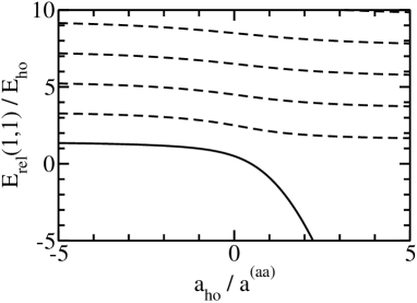
Figure 1: Relative $s$-wave energies $E_{\mathrm{rel}}(1,1)$ of the trapped atom-atom system, obtained by solving Eq. (15) for $k=aa$, as a function of $a_{\mathrm{ho}}/a^{(aa)}$. The lowest $s$-wave eigenenergy (solid line) is referred to as $E_{\mathrm{dimer}}$ in the text. Here, $E_{\mathrm{ho}}$ denotes the harmonic oscillator energy, $E_{\mathrm{ho}}=\hbar\omega$.

shows the relative eigenenergies $E_{\mathrm{rel}}(1,1)$ obtained by solving Eq. (15) for $k=aa$ as a function of $a_{\mathrm{ho}}/a^{(aa)}$ [in this case, $E_{\mathrm{eff}}=E_{\mathrm{rel}}(1,1)$ and $\mu^{(k)}=m/2$]. From Eq. (15) one finds at unitarity $E_{\mathrm{unit,rel}}(1,1)=(2n_{\mathrm{eff}}+1/2)\hbar\omega$ for $s$-wave states. The eigenenergies $E_{\mathrm{eff}}$ of the effective atom-dimer and dimer-dimer systems can be obtained from Fig. 1 by scaling the horizontal axis appropriately.

Within the effective two-particle model, the relative energies $E_{\mathrm{rel}}(2,1)$ and $E_{\mathrm{rel}}(2,2)$ of the three- and four-fermion systems are given by $E_{\mathrm{rel}}(2,1)=E_{\mathrm{eff}}+E_{\mathrm{dimer}}$ and $E_{\mathrm{rel}}(2,2)=E_{\mathrm{eff}}+2E_{\mathrm{dimer}}$, where the second term on the right hand sides accounts for the internal molecular binding energy of the dimer(s) in the presence of the trap stec07b ; stec08 . $E_{\mathrm{dimer}}$ is given by the lowest energy solution of Eq. (15) with $k=aa$ and $\mu^{(aa)}=m/2$ (see solid line in Fig. 1). For $a^{(aa)}\ll a_{\mathrm{ho}}$, the size of the dimer—given to first order by $a^{(aa)}$—is much smaller than the trap size and $E_{\mathrm{dimer}}$ approaches the free-space result $E_{\mathrm{dimer}}^{\mathrm{free}}=-\hbar^{2}/[m(a^{(aa)})^{2}]$. As $a^{(aa)}$ increases, the role of the confinement becomes increasingly more important and the lowest energy solution of Eq. (15) starts to deviate from $E_{\mathrm{dimer}}^{\mathrm{free}}$. Expanding Eq. (15) about the non-interacting energies $(2n_{\mathrm{eff}}+3/2)\hbar\omega$, the $s$-wave energies $E_{\mathrm{eff}}$ can be approximated as busc98

$$E_{\mathrm{eff}}\approx$$

$$\left(2n_{\mathrm{eff}}+3/2+\frac{2\Gamma(n_{\mathrm{eff}}+3/2)}{\sqrt{\pi}\Gamma(n_{\mathrm{eff}}+1)\Gamma(3/2)}\frac{a^{(k)}}{a_{\mathrm{ho},\mu}^{(k)}}\right)\hbar\omega$$ (17)

for small $|a^{(k)}|$. Alternatively, this result can be obtained by treating the atom-dimer and dimer-dimer interactions within first order perturbation theory.

Lastly, we discuss the angular momentum $L_{\mathrm{rel}}$ of the three- and four-fermion systems implied by the effective model Hamiltonian $H^{\mathrm{eff}}$. If $E_{\mathrm{eff}}$ is taken to be one of the positive energy solutions of Eq. (15), then the total relative angular momentum $L_{\mathrm{rel}}$ of the three- and four-fermion systems is $0$ and the states have natural parity, i.e., $\Pi_{\mathrm{rel}}=+1$. If $E_{\mathrm{eff}}$ is taken to be an eigenenergy of $H^{\mathrm{eff}}$ with finite angular momentum $l_{\mathrm{eff}}$, i.e., $E_{\mathrm{eff}}=(2n_{\mathrm{eff}}+l_{\mathrm{eff}}+3/2)\hbar\omega$ with $n_{\mathrm{eff}}=0,1,\cdots$, then the total relative angular momentum of the three- and four-fermion systems is $L_{\mathrm{rel}}=l_{\mathrm{eff}}$ and the states have, as above, natural parity, i.e., $\Pi_{\mathrm{rel}}=(-1)^{L_{\mathrm{rel}}}$. These observations are used below to interpret Figs. 5 and 10.

II.2 Hyperspherical Coordinate Approach

The hyperspherical framework serves two distinct purposes in this paper. It allows for (i) the construction of non-interacting wave functions with good quantum numbers and (ii) the classification of the energy spectrum at unitarity. This section first treats the non-interacting Fermi gas using hyperspherical coordinates and then reviews how the formalism, with some modifications, carries over to the infinitely strongly-interacting unitary Fermi gas.

To construct the eigenfunctions of the non-interacting Fermi gas, we write the many-body Hamiltonian $H^{\mathrm{ni}}$, Eq. (2), in hyperspherical coordinates aver89 ; lin95 ; bohn98 ; timo02 ; timo04 ; ripe05 ; wern06 ; ritt06 ; reviewgreen . We first separate off the center-of-mass vector $\vec{R}_{\mathrm{cm}}$ and then divide the remaining $3N-3$ coordinates into $3N-4$ hyperangles, collectively denoted by $\vec{\Omega}$ (see below for their definition), and the hyperradius $R$,

$$R^{2}=\frac{1}{N}\sum_{j=1}^{N}(\vec{r}_{j}-\vec{R}_{\mathrm{cm}})^{2}.$$ (18)

Using these coordinates, the Hamiltonian $H^{\mathrm{ni}}$ can be written as

$$H^{\mathrm{ni}}=H^{\mathrm{cm}}-\frac{\hbar^{2}}{2M}\left(\frac{\partial^{2}}{\partial R^{2}}+\frac{3N-4}{R}\frac{\partial}{\partial R}\right)+$$

$$\frac{\Lambda^{2}}{2MR^{2}}+\frac{1}{2}M\omega^{2}R^{2},$$ (19)

where the center-of-mass Hamiltonian $H^{\mathrm{cm}}$ is given by

$$H^{\mathrm{cm}}=\frac{-\hbar^{2}}{2M}\nabla_{\vec{R}_{\mathrm{cm}}}^{2}+\frac{1}{2}M\omega^{2}R_{\mathrm{cm}}^{2}$$ (20)

and $M$ denotes the total mass of the system, i.e., $M=Nm$. In Eq. (II.2), $\Lambda$ denotes the so-called grand angular momentum operator aver89 that accounts for the kinetic energy associated with the hyperangles $\vec{\Omega}$. The eigenfunctions $\psi^{\mathrm{ni}}$ of the Hamiltonian $H^{\mathrm{ni}}$ separate (see, e.g., Refs. aver89 ; wern06 ; ritt06 ),

$$\psi^{\mathrm{ni}}(\vec{r}_{1},\cdots,\vec{r}_{N})=$$

$$G_{N_{\mathrm{cm}},L_{\mathrm{cm}},M_{\mathrm{cm}}}(\vec{R}_{\mathrm{cm}})F_{q,\lambda}(R)\Phi_{\lambda,\chi}(\vec{\Omega}).$$ (21)

Here, the center-of-mass functions $G_{N_{\mathrm{cm}},L_{\mathrm{cm}},M_{\mathrm{cm}}}(\vec{R}_{\mathrm{cm}})$ are eigenfunctions of $H^{\mathrm{cm}}$, i.e., three-dimensional harmonic oscillator functions in the center-of-mass vector $\vec{R}_{\mathrm{cm}}$, with eigenenergies $E_{\mathrm{cm}}=(2N_{\mathrm{cm}}+L_{\mathrm{cm}}+3/2)\hbar\omega$, where $N_{\mathrm{cm}}=0,1,\cdots$, $L_{\mathrm{cm}}=0,1,\cdots$ and $M_{\mathrm{cm}}=-L_{\mathrm{cm}},-L_{\mathrm{cm}}+1,\cdots,L_{\mathrm{cm}}$. The hyperspherical harmonics $\Phi_{\lambda,\chi}(\vec{\Omega})$, or so-called channel functions, are eigenfunctions of the operator $\Lambda^{2}$ aver89 ,

$$\Lambda^{2}\Phi_{\lambda,\chi}(\vec{\Omega})=\hbar^{2}\lambda(\lambda+3N-5)\Phi_{\lambda,\chi}(\vec{\Omega}),$$ (22)

where $\lambda$ can take the values $0,1,2,\cdots$. The quantum number $\chi$ denotes the degeneracy for each $\lambda$ aver89 ,

$$\chi=\frac{(3N+2\lambda-5)(3N+\lambda-6)!}{\lambda!(3N-5)}.$$ (23)

In deriving Eq. (23), no symmetry constraints have been enforced. Below, we discuss the construction of the hyperspherical harmonics and the reduction of the degeneracy $\chi$ due to symmetry constraints for the three- and four-fermion systems. Since the center-of-mass coordinates and the hyperradius are unchanged under the exchange of $\vec{r}_{j}$ and $\vec{r}_{k}$ ($j,k=1,\cdots,N$), the symmetry-constraints only effect the $\Phi_{\lambda,\chi}(\vec{\Omega})$ and neither $G_{N_{\mathrm{cm}},L_{\mathrm{cm}},M_{\mathrm{cm}}}(\vec{R}_{\mathrm{cm}})$ nor $F_{q,\lambda}(R)$.

Plugging Eq. (II.2) into the Schrödinger equation $H^{\mathrm{ni}}\psi^{\mathrm{ni}}=E_{\mathrm{ni}}(N_{\uparrow},N_{\downarrow})\psi^{\mathrm{ni}}$ and dividing out the center-of-mass and hyperangular contributions, we obtain an effective hyperradial Schrödinger equation wern06 ; ritt06 ,

$$\left(-\frac{\hbar^{2}}{2M}\frac{\partial^{2}}{\partial R^{2}}+\frac{\hbar^{2}K_{\mathrm{ni}}(K_{\mathrm{ni}}+1)}{2MR^{2}}+\frac{1}{2}M\omega^{2}R^{2}\right)\bar{\mathrm{F}}_{q,\lambda}(R)$$

$$=\big{[}E_{\mathrm{ni}}(N_{\uparrow},N_{\downarrow})-E_{\mathrm{cm}}\big{]}\bar{\mathrm{F}}_{q,\lambda}(R),$$ (24)

where

$$\bar{\mathrm{F}}_{q,\lambda}(R)=R^{(3N-4)/2}F_{q,\lambda}(R)$$ (25)

and

$$K_{\mathrm{ni}}=\lambda+\frac{3N-6}{2}.$$ (26)

Noticing that the effective hyperradial Schrödinger equation, Eq. (II.2), is formally identical to the Schrödinger equation for the three-dimensional harmonic oscillator with angular momentum $K_{\mathrm{ni}}$ wern06 ; ritt06 , the eigenenergies $E_{\mathrm{ni,rel}}$, $E_{\mathrm{ni,rel}}(N_{\uparrow},N_{\downarrow})=E_{\mathrm{ni}}(N_{\uparrow},N_{\downarrow})-E_{\mathrm{cm}}$, and the corresponding eigenfunctions $\bar{\mathrm{F}}_{q,\lambda}(R)$ are readily written down,

$$E_{\mathrm{ni,rel}}=\left(2q+K_{\mathrm{ni}}+\frac{3}{2}\right)\hbar\omega$$ (27)

with $q=0,1,\cdots$ and

$$\bar{\mathrm{F}}_{q,\lambda}(R)=$$

$$N_{qK_{\mathrm{ni}}}R^{K_{\mathrm{ni}}+1}\exp\left(-\frac{R^{2}}{2a_{M}^{2}}\right)L_{q}^{(K_{\mathrm{ni}}+1/2)}\left(\frac{R^{2}}{a_{M}^{2}}\right).$$ (28)

The normalization constant $N_{qK_{\mathrm{ni}}}$ is chosen such that

$$\int_{0}^{\infty}|\bar{\mathrm{F}}_{q,\lambda}(R)|^{2}dR=1,$$ (29)

leading to

$$N_{qK_{\mathrm{ni}}}=\sqrt{\frac{2^{K_{\mathrm{ni}}+2}}{(2K_{\mathrm{ni}}+1)!!\sqrt{\pi}L_{q}^{(K_{\mathrm{ni}}+1/2)}(0)a_{\mathrm{ho},M}^{2K_{\mathrm{ni}}+3}}},$$ (30)

where $L_{q}^{(K_{\mathrm{ni}}+1/2)}$ denotes the associated Laguerre polynomial. The harmonic oscillator length $a_{\mathrm{ho},M}$, $a_{\mathrm{ho},M}=\sqrt{\hbar/(M\omega)}$, can be interpreted as being associated with an effective mass $M$ particle that moves along the hyperradial coordinate $R$. The quantity $K_{\mathrm{ni}}$ depends on $\lambda$ and can be thought of as an effective angular momentum quantum number; it should be noted, though, that the $K_{\mathrm{ni}}$ are, in general, neither equal to the total angular momentum $L_{tot}$ nor equal to the relative angular momentum $L_{\mathrm{rel}}$ of the two-component Fermi gas.

The explicit construction of the hyperspherical harmonics $\Phi_{\lambda,\chi}(\vec{\Omega})$ requires the hyperangles $\vec{\Omega}$ to be specified. The hyperangles $\vec{\Omega}$ can be defined in many different ways and here we employ definitions that allow for a straightforward anti-symmetrization of the $\Phi_{\lambda,\chi}(\vec{\Omega})$. To this end, we introduce a set of mass scaled Jacobi vectors $\vec{u}_{i}$, $i=1,\cdots,N-1$, where aver89 ; lin95

$$\vec{u}_{i}=\sqrt{\frac{M}{\mu_{i}}}\vec{\rho}_{i}.$$ (31)

Table 1

Table 1: Definition of the Jacobi vectors $\vec{\rho}_{i}$ and the associated reduced masses $\mu_{i}$ used in our construction of the hyperspherical harmonics $\Phi_{\lambda,\chi}$ for the two-component equal-mass atomic Fermi gas with $(N_{\uparrow},N_{\downarrow})=(2,1)$ and $(2,2)$.

$(N_{\uparrow},N_{\downarrow})$	$\vec{\rho}_{1}$	$\vec{\rho}_{2}$	$\vec{\rho}_{3}$	$\mu_{1}$	$\mu_{2}$	$\mu_{3}$
$(2,1)$	$\vec{r}_{1}-\vec{r}_{2}$	$\frac{\vec{r}_{1}+\vec{r}_{2}}{2}-\vec{r}_{3}$		$\frac{m}{2}$	$\frac{2m}{3}$
$(2,2)$	$\vec{r}_{1}-\vec{r}_{2}$	$\vec{r}_{3}-\vec{r}_{4}$	$\frac{\vec{r}_{1}+\vec{r}_{2}}{2}-\frac{\vec{r}_{3}+\vec{r}_{4}}{2}$	$\frac{m}{2}$	$\frac{m}{2}$	$m$

lists the Jacobi coordinates $\vec{\rho}_{i}$ and the associated reduced masses $\mu_{i}$ employed in this paper for the treatment of atomic two-component equal-mass three- and four-fermion systems. These Jacobi vectors have particularly convenient properties under the exchange of identical fermions. For the $(N_{\uparrow},N_{\downarrow})=(2,1)$ system, the Jacobi vector $\vec{\rho}_{1}$ changes sign under the exchange of the two spin-up fermions while $\vec{\rho}_{2}$ remains unchanged. For the $(N_{\uparrow},N_{\downarrow})=(2,2)$ system, the exchange of the two spin-up fermions leads to a sign change of $\vec{\rho}_{1}$ while $\vec{\rho}_{2}$ and $\vec{\rho}_{3}$ remain unchanged, the exchange of the two spin-down fermions leads to a sign change of $\vec{\rho}_{2}$ while $\vec{\rho}_{1}$ and $\vec{\rho}_{3}$ remain unchanged, and the simultaneous exchange of the two spin-up fermions and the two spin-down fermions leads to a sign change of $\vec{\rho}_{1}$ and $\vec{\rho}_{2}$ while $\vec{\rho}_{3}$ remains unchanged. These properties of the Jacobi vectors make the construction of properly anti-symmetrized hyperspherical harmonics $\Phi_{\lambda,\chi}(\vec{\Omega})$ for the three- and four-fermion systems comparatively simple. In terms of the mass-scaled Jacobi vectors $\vec{u}_{i}$, the $3N-4$ hyperspherical angles $\vec{\Omega}$ are defined as $\vec{\Omega}=(\vec{u}_{1}/R,\cdots,\vec{u}_{N-1}/R)$ and the hyperradius $R$, Eq. (18), can be rewritten as $R^{2}=\sum_{i=1}^{N-1}\vec{u}_{i}^{2}$ aver89 ; lin95 .

Following Avery aver89 , we construct a complete set of hyperspherical harmonics $\Phi_{\lambda,\chi}(\vec{\Omega})$, which are simultaneous eigenfunctions of the operators $\Lambda^{2}$, $L^{2}_{\mathrm{rel}}$, $L_{\mathrm{rel},z}$ and $\Pi_{\mathrm{rel}}$. Although the explicit functional forms of the $\Phi_{\lambda,\chi}(\vec{\Omega})$ are needed in our perturbative treatment, we restrict ourselves here to summarizing the degeneracies of the non-interacting eigenfunctions for the $(N_{\uparrow},N_{\downarrow})=(2,1)$ and $(2,2)$ systems (see Tables 2

Table 2: Characterization of the hyperspherical harmonics $\Phi_{\lambda,\chi}(\vec{\Omega})$ for the $(N_{\uparrow},N_{\downarrow})=(2,1)$ system with $\lambda\leq 5$. In determining $\chi$, only hyperspherical harmonics that change sign under the exchange of the two spin-up atoms are counted.

$\lambda$	$\chi$	$K_{\mathrm{ni}}$	$L_{\mathrm{rel}}$	${\Pi}_{\mathrm{rel}}$
$1$	3	5/2	1	$-1$
2	5	7/2	2	$+1$
2	3	7/2	1	$+1$
2	1	7/2	0	$+1$
3	14	9/2	3	$-1$
3	5	9/2	2	$-1$
3	6	9/2	1	$-1$
4	18	11/2	4	$+1$
4	14	11/2	3	$+1$
4	15	11/2	2	$+1$
4	3	11/2	1	$+1$
4	1	11/2	0	$+1$
5	33	13/2	5	$-1$
5	18	13/2	4	$-1$
5	28	13/2	3	$-1$
5	10	13/2	2	$-1$
5	9	13/2	1	$-1$

and

Table 3: Characterization of the hyperspherical harmonics $\Phi_{\lambda,\chi}(\vec{\Omega})$ for the $(N_{\uparrow},N_{\downarrow})=(2,2)$ system with $\lambda\leq 5$. In determining $\chi$, only hyperspherical harmonics that change sign under the exchange of the two spin-up atoms and the two spin-down atoms are counted.

$\lambda$	$\chi$	$K_{\mathrm{ni}}$	$L_{\mathrm{rel}}$	${\Pi}_{\mathrm{rel}}$
$2$	5	5	2	$+1$
$2$	3	5	1	$+1$
$2$	1	5	0	$+1$
$3$	7	6	3	$-1$
$3$	10	6	2	$-1$
$3$	9	6	1	$-1$
$3$	1	6	0	$-1$
$4$	27	7	4	$+1$
$4$	28	7	3	$+1$
$4$	35	7	2	$+1$
$4$	12	7	1	$+1$
$4$	3	7	0	$+1$
$5$	33	8	5	$-1$
$5$	54	8	4	$-1$
$5$	77	8	3	$-1$
$5$	50	8	2	$-1$
$5$	27	8	1	$-1$
$5$	2	8	0	$-1$

3).

Table 2 shows the degeneracies $\chi$ and quantum numbers of the hyperspherical harmonics for the $(N_{\uparrow},N_{\downarrow})=(2,1)$ system with $\lambda$ up to $5$; in constructing Table 2, only hyperspherical harmonics that change sign under the exchange of the two spin-up atoms have been counted. This symmetry constraint reduces the degeneracy of each $\lambda$ manifold tremendously. Equation (23)—applicable to a system without symmetry constraints—gives 1, 6, 20, and 50 for $\lambda=0,1,2$ and 3, while Table 2 shows that the degeneracies are reduced to 0, 3, 9 and 25. Table 2 can be readily constructed by considering the angular momentum operators $\vec{l}_{1}$ and $\vec{l}_{2}$ associated with the Jacobi vectors $\vec{\rho}_{1}$ and $\vec{\rho}_{2}$, and by taking into account that $\vec{l}_{1}$ and $\vec{l}_{2}$ couple to $\vec{L}_{\mathrm{rel}}$ aver89 . Since $\vec{\rho}_{1}$ is the Jacobi vector that connects the two spin-up fermions, $l_{1}$ can only take odd values; $l_{2}$, in contrast, is not restricted by symmetry constraints, implying $l_{2}=0,1,\cdots$. For a given $\lambda$, the allowed $(l_{1},l_{2})$ combinations are determined by $\lambda=l_{1}+l_{2}+2p$, where $p=0,1,\cdots$ aver89 ; reviewgreen . Since the $(l_{1},l_{2})=(0,0)$ combination is symmetry-forbidden, the smallest allowed $\lambda$ value is $1$. For $\lambda=1$, the only possible $(l_{1},l_{2})$ combination is $(1,0)$, resulting in $L_{\mathrm{rel}}=1$, $\Pi_{\mathrm{rel}}=(-1)^{l_{1}+l_{2}}=-1$ and a degeneracy of $\chi=3$ (corresponding to three different projection quantum numbers $M_{L}$). For $\lambda=2$, the only possible $(l_{1},l_{2})$ combination is $(1,1)$, leading to $L_{\mathrm{rel}}=0,1,2$ and $\Pi_{\mathrm{rel}}=+1$. The degeneracy $\chi$ is 9 (1, 3 and 5 states for $L_{\mathrm{rel}}=0$, 1 and 2, respectively). For $\lambda=3$, the allowed $(l_{1},l_{2})$ combinations are $(3,0)$, $(1,2)$ and $(1,0)$, leading to $L_{\mathrm{rel}}=3$ (7 states), $L_{\mathrm{rel}}=3,2,1$ (15 states) and $L_{\mathrm{rel}}=1$ (3 states), respectively; thus, the degeneracy $\chi$ is 25. Following this reasoning, the remaining entries in Table 2 can be verified.

Table 3 summarizes the degeneracies and quantum numbers for the $(N_{\uparrow},N_{\downarrow})=(2,2)$ system. Similarly to the three-fermion case, Table 3 is constructed by realizing that the angular momentum quantum numbers $l_{1}$ and $l_{2}$ associated with the Jacobi vectors $\vec{\rho}_{1}$ and $\vec{\rho}_{2}$ can only take odd values and that $l_{3}$, where $l_{3}$ denotes the angular momentum quantum number associated with the Jacobi vector $\vec{\rho}_{3}$, can take any value. For a given $\lambda$, the allowed $(l_{1},l_{2},l_{3})$ combinations are determined by $\lambda=l_{1}+l_{2}+l_{3}+2p+2q$, where $p,q=0,1,\cdots$ aver89 ; reviewgreen . Since both $l_{1}$ and $l_{2}$ have to be odd, the smallest allowed $\lambda$ value is 2. In this case, $l_{1}=l_{2}=1$ and $l_{3}=0$. The $\lambda=2$ manifold thus consists of nine states [$\vec{l}_{1}$, $\vec{l}_{2}$ and $\vec{l}_{3}$ can couple so that $L_{\mathrm{rel}}=2$ (5 states), $1$ (3 states) and 0 (1 state)]. For $\lambda=3$, the only possibility is $(l_{1},l_{2},l_{3})=(1,1,1)$, implying $27$ states. The angular momenta corresponding to these 27 states can be obtained by first coupling $\vec{l}_{1}$ and $\vec{l}_{2}$ to an intermediate angular momentum vector with quantum number $2$, 1 or 0, and then coupling the intermediate angular momentum vector and $\vec{l}_{3}$ to obtain $\vec{L}_{\mathrm{rel}}$. The higher $\lambda$ manifolds are treated following the same scheme.

Knowing the allowed $\lambda$ and $\chi$ values, the degeneracy $g_{\mathrm{ni,rel}}$ of a given relative energy $E_{\mathrm{ni,rel}}(N_{\uparrow},N_{\downarrow})$ of the non-interacting trapped Fermi gas can be easily determined using Eq. (26) and Eq. (27). These degeneracies are summarized in the second column of Tables 4

Table 4: Coefficients $c^{(1)}$ for Fermi gas with $(N_{\uparrow},N_{\downarrow})=(2,1)$. The $c^{(1)}$ are defined through $E^{(1)}=c^{(1)}(2\pi)^{-1/2}\hbar\omega a^{(aa)}/a_{\mathrm{ho}}$.

$E_{\mathrm{ni,rel}}/(\hbar\omega)$	$g_{\mathrm{ni,rel}}$	$L_{\mathrm{rel}}$	${\Pi}_{\mathrm{rel}}$	$c^{(1)}$
$4$	3	1	$-1$	3
$5$	5	2	$+1$	3/2
$5$	3	1	$+1$	0
$5$	1	0	$+1$	15/4
$6$	7	3	$-1$	9/4
$6$	7	3	$-1$	0
$6$	5	2	$-1$	0
$6$	3	1	$-1$	$\frac{3}{16}(13+\sqrt{41})$
$6$	3	1	$-1$	$\frac{3}{16}(13-\sqrt{41})$
$6$	3	1	$-1$	0

and 5 for the three- and four-fermion

Table 5: Coefficients $c^{(1)}$ for Fermi gas with $(N_{\uparrow},N_{\downarrow})=(2,2)$. The $c^{(1)}$ are defined through $E^{(1)}=c^{(1)}(2\pi)^{-1/2}\hbar\omega a^{(aa)}/a_{\mathrm{ho}}$.

$E_{\mathrm{ni,rel}}/(\hbar\omega)$	$g_{\mathrm{ni,rel}}$	$L_{\mathrm{rel}}$	${\Pi}_{\mathrm{rel}}$	$c^{(1)}$
13/2	5	2	$+1$	5
13/2	3	1	$+1$	4
13/2	1	0	$+1$	13/2
15/2	7	3	$-1$	7/2
15/2	5	2	$-1$	3
15/2	5	2	$-1$	2
15/2	3	1	$-1$	5
15/2	3	1	$-1$	$\frac{1}{8}(29+\sqrt{41})$
15/2	3	1	$-1$	$\frac{1}{8}(29-\sqrt{41})$
15/2	1	0	$-1$	0
17/2	9	4	$+1$	$\frac{1}{8}(27+\sqrt{73})$
17/2	9	4	$+1$	5/2
17/2	9	4	$+1$	$\frac{1}{8}(27-\sqrt{73})$
17/2	7	3	$+1$	$\frac{1}{4}(9+\sqrt{17})$
17/2	7	3	$+1$	3
17/2	7	3	$+1$	$\frac{1}{4}(9-\sqrt{17})$
17/2	7	3	$+1$	0
17/2	5	2	$+1$	5.89252
17/2	5	2	$+1$	5.31030
17/2	5	2	$+1$	4.61321
17/2	5	2	$+1$	3.21783
17/2	5	2	$+1$	3.21549
17/2	5	2	$+1$	1.92129
17/2	5	2	$+1$	1.45435
17/2	5	2	$+1$	0
17/2	3	1	$+1$	4.50566
17/2	3	1	$+1$	3
17/2	3	1	$+1$	1.73167
17/2	3	1	$+1$	0.512668
17/2	3	1	$+1$	0
17/2	1	0	$+1$	7.40848
17/2	1	0	$+1$	6.98138
17/2	1	0	$+1$	15/4
17/2	1	0	$+1$	2.89139

systems, respectively. Alternatively timo02 ; ritt06 , the relative energy $E_{\mathrm{ni,rel}}(N_{\uparrow},N_{\downarrow})$ of the non-interacting three- and four-fermion systems can be written as $E_{\mathrm{ni,rel}}(N_{\uparrow},N_{\downarrow})=\sum_{j=1}^{N-1}(2n_{j}+l_{j}+3/2)\hbar\omega$, where $n_{j}=0,1,\cdots$ and where the allowed angular momentum quantum numbers $l_{j}$ are determined by the symmetry requirements (see above). Counting the possible combinations of $l_{j}$ and $n_{j}$ values and taking the $(2l_{j}+1)$ degeneracy associated with each $l_{j}$ into account, gives the same results as those reported in the second column of Tables 4 and 5, and also allows—using Eqs. (26) and (27)—for an independent determination of the $\lambda$ and $\chi$ values given in the first two columns of Tables 2 and 3.

So far, we have discussed the hyperspherical framework for the non-interacting two-component Fermi gas. We now review the modifications needed when applying this framework to the infinitely strongly-interacting unitary gas with zero-range two-body interactions. The zero-range two-body potential with infinite $a^{(aa)}$ does not establish a meaningful length scale, leaving the oscillator length $a_{\mathrm{ho}}$ as the only length scale in the problem. Using scale invariance arguments, it has been shown wern06 that a diverging $s$-wave scattering length $a^{(aa)}$ implies that the wave function $\psi^{\mathrm{unit}}(\vec{r}_{1},\cdots,\vec{r}_{N})$ at unitarity separates in the same way as that of the non-interacting system [see Eq. (II.2)]. It follows that Eq. (II.2) applies not only to the non-interacting gas but also to the unitary gas if $K_{\mathrm{ni}}$ is replaced by $K_{\mathrm{unit}}$ and if $\lambda$ is reinterpreted as the eigenvalue of the hyperangular eigenequation that takes the two-body interactions into account. In the following, we use $K_{\mathrm{unit}}$ to denote the effective angular momentum of the unitary gas. Note that $K_{\mathrm{unit}}$ depends on the eigenvalue of the hyperangular eigenequation, i.e., there exists a $K_{\mathrm{unit}}$ for each channel function $\Phi_{\lambda,\chi}(\vec{\Omega})$; for notational convenience, we do not explicitly indicate the dependence of $K_{\mathrm{unit}}$ on the hyperangular quantum numbers.

The coefficients $K_{\mathrm{unit}}$ have beeen obtained for all states of the three-fermion system wern06a (see also Refs. efim71 ; efim73 ; dinc05 for earlier work) and for the lowest 20 states with $(L_{\mathrm{rel}},\Pi_{\mathrm{rel}})=(0,+1)$ of the four-fermion system stec09 by solving the hyperangular Schrödinger equation that includes the two-body interactions (see also Ref. blum07 ). The relative eigenenergies $E_{\mathrm{unit,rel}}$ of the unitary gas are, similarly to the non-interacting case, given by wern06

$$E_{\mathrm{unit,rel}}=(2q+K_{\mathrm{unit}}+3/2)\hbar\omega,$$ (32)

and Eqs. (II.2)-(30) remain valid if $K_{\mathrm{ni}}$ is replaced by $K_{\mathrm{unit}}$ (and if $\lambda$ is reinterpreted as discussed above). In Sec. III, we determine a number of $K_{\mathrm{unit}}$ coefficients by solving the full relative Schrödinger equation of the four-fermion system for various $L_{\mathrm{rel}}>0$ and by then comparing the resulting energy with the right hand side of Eq. (32). Lastly, we note that Eq. (32) implies that the excitation spectrum of the trapped unitary two-component Fermi gas contains ladders of excitation frequencies that are integer multiples of $2\hbar\omega$, independent of the actual values of $K_{\mathrm{unit}}$ tan04 ; cast04 ; wern06 .

II.3 Numerical treatment of the three-fermion system: Lippmann-Schwinger equation

The trapped three-fermion problem with zero-range interactions and arbitrary $s$-wave scattering length $a^{(aa)}$ has been solved using a number of different semi-analytical and numerical approaches kest07 ; stet07 ; stec08 . Here, we replace the regularized zero-range pseudo-potential $V_{\mathrm{F,reg}}^{(aa)}(\vec{r})$, which describes the interactions between atoms with opposite spins, by the corresponding Bethe-Peierls boundary condition and employ an approach developed by Kestner and Duan kest07 that is based on the Lippmann-Schwinger equation. This approach reduces the three-body problem to solving a set of coupled equations kest07 ,

$$\frac{2\Gamma\left(-\nu_{j}\right)}{\Gamma\left(-\nu_{j}-\frac{1}{2}\right)}c_{j}+\sum_{k=1}^{B}d_{jk}c_{k}=\left(\frac{a_{\mathrm{ho},\mu}^{(aa)}}{a^{(aa)}}\right)c_{j},$$ (33)

for the eigenvector $\vec{c}$, $\vec{c}=(c_{1},\cdots,c_{B})$, and the eigenvalue $(a^{(aa)}/a_{\mathrm{ho},\mu}^{(aa)})^{-1}$. In Eq. (33), the $\nu_{j}$ denote non-integer quantum numbers that depend on $E_{\mathrm{rel}}(2,1)$ and the $d_{jk}$ dimensionless matrix elements. Their definitions are given in Refs. kest07 ; liu09 .

In the $B\rightarrow\infty$ limit, Eq. (33) gives the exact three-fermion energy spectrum. For each $E_{\mathrm{rel}}(2,1)$, there exist multiple $\vec{c}$ and $a^{(aa)}$ that solve Eq. (33). Thus, Eq. (33) can be interpreted as a matrix equation with eigenvector matrix $\underline{c}=(\vec{c}_{1},\cdots,\vec{c}_{B})$ and eigenvalue vector $((a^{(aa)})_{1},\cdots,(a^{(aa)})_{B})$. The solutions obtained by solving Eq. (33) belong to three-fermion states with natural parity. For the three-fermion system, unnatural parity states are not affected by the $s$-wave zero-range interactions and coincide with those of the non-interacting system. For each $L_{\mathrm{rel}}$, we solve the matrix problem for different $B$, $B\leq 50$. For positive $E_{\mathrm{rel}}(2,1)$, our results presented in Sec. III.1 are obtained using $B=50$. For negative $E_{\mathrm{rel}}(2,1)$, we use somewhat smaller $B$ values; we have checked through extrapolation to the $B\rightarrow\infty$ limit that the three-fermion energies obtained in this manner are highly accurate. We find, e.g., that the eigenenergies at unitarity obtained by the numerical approach based on the Lippmann-Schwinger equation kest07 agree to better than 0.01% with those obtained by solving the transcendental equation derived by Werner and Castin wern06a .

II.4 Numerical treatment of the four-fermion system: Stochastic variational approach

To determine the energy spectrum of two-component Fermi gases with $(N_{\uparrow},N_{\downarrow})=(2,2)$ under spherically symmetric harmonic confinement, we employ the stochastic variational approach varg95 ; varg01 ; cgbook ; sore05 ; stec07c ; stec07b ; stec08 . Our implementation separates off the center-of-mass degrees of freedom $\vec{R}_{\mathrm{cm}}$, defines a set of $N-1$ Jacobi coordinates $\vec{x}$, $\vec{x}=(\vec{\rho}_{1},\cdots,\vec{\rho}_{N-1})$, and expands the relative wave function $\psi_{\mathrm{rel}}(\vec{x})$ in terms of the basis functions $\varphi_{k}(\vec{x})$,

$$\psi_{\mathrm{rel}}(\vec{x})=\sum_{k=1}^{B}{\cal{A}}\left[c_{k}\varphi_{k}(\vec{x})\right],$$ (34)

where the anti-symmetrization operator ${\cal{A}}$ can be written as ${\cal{A}}=1-P_{12}-P_{34}+P_{12}P_{34}$ for the $(N_{\uparrow},N_{\downarrow})=(2,2)$ system. In Eq. (34), the $c_{k}$ denote expansion coefficients. We parametrize the two-body potential $V_{\mathrm{tb}}$ by a spherically symmetric attractive Gaussian with depth $V_{0}$ ($V_{0}>0$) and range $r_{0}$,

$$V_{\mathrm{G}}(\vec{r})=-V_{0}\exp\left[-\left(\frac{r}{\sqrt{2}r_{0}}\right)^{2}\right];$$ (35)

this interaction potential is convenient since the matrix elements $\langle\varphi_{j}|V_{\mathrm{G}}|\varphi_{k}\rangle$ are—for the $\varphi_{k}$ employed in this work—known analytically cgbook (see below for the definition of the $\varphi_{k}$). For a given range $r_{0}$, we adjust the depth $V_{0}$ such that $V_{\mathrm{G}}$ reproduces the desired $s$-wave scattering length $a^{(aa)}$. For negative (positive) $a^{(aa)}$, we restrict ourselves to parameter combinations for which $V_{\mathrm{G}}(\vec{r})$ supports no (one) $s$-wave free-space bound state. For each $a^{(aa)}$, we consider a number of different ranges $r_{0}$, $r_{0}\ll a_{\mathrm{ho}}$, and extrapolate to the $r_{0}\rightarrow 0$ limit (see Sec. III.2 for details).

We employ two different classes of non-orthogonal basis functions $\varphi_{k}$. For both classes, the Hamiltonian matrix elements and overlap matrix elements are known analytically cgbook , thus reducing the problem of finding the eigenenergies and eigenfunctions to diagonalizing a generalized eigenvalue problem. The first class of basis functions $\varphi_{k}(\vec{x})$ has well defined angular momentum $L_{\mathrm{rel}}$ and natural parity, while the latter class has neither well defined angular momentum $L_{\mathrm{rel}}$ nor well defined parity $\Pi_{\mathrm{rel}}$.

To describe natural parity states with well defined angular momentum $L_{\mathrm{rel}}$ and corresponding projection quantum number $M_{L}$, we employ the following basis functions cgbook ,

$$\varphi_{k}(\vec{x})=|\vec{v}^{(k)}|^{L_{\mathrm{rel}}}{Y}_{L_{\mathrm{rel}}M_{L}}(\hat{v}^{(k)})\exp\left(-\frac{1}{2}\vec{x}^{T}\underline{A}^{(k)}\vec{x}\right),$$ (36)

where

$$\vec{v}^{(k)}=\sum_{j=1}^{N-1}u_{j}^{(k)}\vec{\rho}_{j}.$$ (37)

Here, the $u_{j}^{(k)}$, $j=1,\cdots,N-1$, define a $(N-1)$-dimensional parameter vector that determines how the angular momentum $L_{\mathrm{rel}}$ is distributed among the $(N-1)$ Jacobi vectors $\vec{\rho}_{j}$. In Eq. (36), $\underline{A}^{(k)}$ denotes a $(N-1)\times(N-1)$-dimensional symmetric matrix, which is described by $N(N-1)/2$ independent parameters. To get a physical interpretation of these parameters, we rewrite the exponent on the right hand side of Eq. (36) in terms of a sum over the square of interparticle distances $r_{ij}$ and $N(N-1)/2$ widths $d_{ij}^{(k)}$,

$$\frac{1}{2}\vec{x}^{T}\underline{A}^{(k)}\vec{x}=\frac{1}{2}\sum_{i=1}^{N-1}\sum_{j=1}^{N-1}A_{ij}^{(k)}\vec{\rho}_{i}\cdot\vec{\rho}_{j}=$$

$$\sum_{i<j}^{N}\left(\frac{r_{ij}}{\sqrt{2}d_{ij}^{(k)}}\right)^{2}.$$ (38)

The explicit relationship between the parameter matrix $\underline{A}^{(k)}$ and the widths $d_{ij}^{(k)}$ ($i<j$) can be determined by expressing the interparticle distance vectors $\vec{r}_{ij}$ in terms of the Jacobi vectors $\vec{x}$ cgbook . Equation (II.4) illustrates that the $d_{ij}^{(k)}$ determine the widths of Gaussian functions in the interparticle distance coordinates. In our calculations, we choose a set of widths $d_{ij}^{(k)}$ for each basis function and construct the matrix $\underline{A}^{(k)}$ from these. The widths $d_{ij}^{(k)}$ themselves are—guided by physical arguments—determined semi-stochastically following the schemes discussed in Refs. cgbook ; stec07c ; stec08 . For the $(N_{\uparrow},N_{\downarrow})=(2,2)$ system with small $r_{0}$ and small positive $a^{(aa)}$, e.g., three-body and four-body bound states are absent petr03 ; petr04aa , implying that at most two of the widths $d_{13}^{(k)}$, $d_{14}^{(k)}$, $d_{23}^{(k)}$ and $d_{24}^{(k)}$ (but not $d_{13}^{(k)}$ and $d_{14}^{(k)}$ simultaneously or $d_{23}^{(k)}$ and $d_{24}^{(k)}$ simultaneously) should be of the order of the two-body range $r_{0}$ for a given $k$. We use the basis functions given in Eq. (36) to determine the eigenenergies of states with vanishing and finite $L_{\mathrm{rel}}$ and natural parity, i.e., $\Pi_{\mathrm{rel}}=(-1)^{L_{\mathrm{rel}}}$.

To describe states with unnatural parity, we employ basis functions $\varphi_{k}$ that are neither eigenfunctions of the angular momentum operator $L_{\mathrm{rel}}$ nor the parity operator $\Pi_{\mathrm{rel}}$ cgbook ,

$$\varphi_{k}(\vec{x})=\exp\left(-\frac{1}{2}\vec{x}^{T}\underline{A}^{(k)}\vec{x}+(\vec{s}^{(k)})^{T}\vec{x}\right).$$ (39)

Here, the quantity $\vec{s}^{(k)}$ consists of $N-1$ three-dimensional parameter vectors and $(\vec{s}^{(k)})^{T}\vec{x}$ is just the dot product between two $3(N-1)$ dimensional vectors. The $3(N-1)$ parameters of $\vec{s}^{(k)}$ are, together with the $N(N-1)/2$ parameters of the matrix $\underline{A}^{(k)}$, optimized semi-stochastically cgbook . Since the basis functions defined in Eq. (39) are neither eigenfunctions of $L_{\mathrm{rel}}$, $M_{L}$ nor $\Pi_{\mathrm{rel}}$, their use allows for the determination of the entire energy spectrum at once. In Sec. III.2, we employ the basis functions given in Eq. (39) to determine the energetically lowest lying unnatural parity state of the four-fermion system with negative $a^{(aa)}$.

Following the schemes outlined, the determination of the four-fermion energies corresponding to unnatural parity states is significantly less numerically efficient than that of natural parity states. This is, of course, not sursprising since only a “fraction” of the basis functions given in Eq. (39) contributes to describing states with the desired angular momentum, projection quantum number and parity.

III Results

This section summarizes the energetics of the three- and four-particle equal-mass Fermi gas.

III.1 Three-fermion system

Figures 2(a) and (b) show the eigenenergies $E_{\mathrm{rel}}(2,1)$

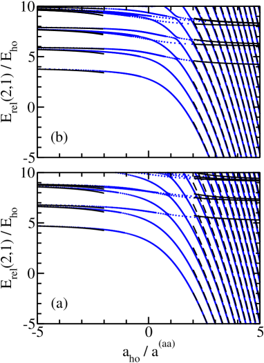
Figure 2: (Color online) Three-fermion energies for (a) $(L_{\mathrm{rel}},\Pi_{\mathrm{rel}})=(0,+1)$ and (b) $(L_{\mathrm{rel}},\Pi_{\mathrm{rel}})=(1,-1)$ as a function of the inverse $s$-wave scattering length $a_{\mathrm{ho}}/a^{(aa)}$. Symbols show the essentially exact zero-range energies obtained by solving Eq. (33). Solid lines show the energies obtained by treating the non-interacting atomic Fermi gas perturbatively for negative and positive $a^{(aa)}$ while dashed lines show the energies obtained by treating the effective atom plus dimer system perturbatively.

for states with natural parity and $L_{\mathrm{rel}}=0$ and $1$ as a function of the inverse scattering length $1/a^{(aa)}$. The symbols show the solutions to the coupled equations, Eq. (33), while the solid and dashed lines are obtained from our perturbative treatments of the atomic Fermi gas and the effective atom plus dimer model, respectively. Note that the perturbative treatment of the atomic Fermi gas (solid lines) describes the energy levels corresponding to gas-like states for negative as well as for positive $a^{(aa)}$ ($|a^{(aa)}|$ small). In the following, we highlight selected characteristics of the three-fermion energy spectrum.

We first consider the weakly-interacting attractive Fermi gas. In the non-interacting limit, $a^{(aa)}\rightarrow 0^{-}$, the ground state has an energy of $E_{\mathrm{ni,rel}}=4\hbar\omega$ and is characterized by $L_{\mathrm{rel}}=1$ and $\Pi_{\mathrm{rel}}=-1$ (see Fig. 2 and Table 4). For the next family of energies with $E_{\mathrm{ni,rel}}=5\hbar\omega$, we have two natural parity states with $L_{\mathrm{rel}}=0$ and $L_{\mathrm{rel}}=2$, respectively, and one unnatural parity state with $L_{\mathrm{rel}}=1$. The fact that the lowest non-interacting $L_{\mathrm{rel}}=0$ state has a higher energy than the lowest non-interacting $L_{\mathrm{rel}}=1$ state can be understood intuitively by realizing that the two like atoms cannot both occupy the lowest single particle state. Within the hyperspherical description, this implies that the $L_{\mathrm{rel}}=0$ state with $\lambda=0$ and $q=0$ is symmetry-forbidden (see Sec. II.2) and that the first symmetry-allowed $L_{\mathrm{rel}}=0$ state, which has $\lambda=2$ and $q=0$, lies $2\hbar\omega$ higher in energy than the symmetry-forbidden $L_{\mathrm{rel}}=0$ state.

The coefficients $c^{(1)}$ that determine the perturbative energy shifts $E^{(1)}$ of the atomic $(N_{\uparrow},N_{\downarrow})=(2,1)$ system are calculated semi-analytically following the scheme outlined in Secs. II.1 and II.2, and reported in the last column of Table 4 for the first three energy families. As already mentioned, the unnatural parity states of the three-fermion system are uneffected by the interactions wern06 ; kest07 ; liu09 . This behavior is specific to zero-range $s$-wave interactions since a finite-range potential allows, in general, for an energy shift due to $p$-wave or other higher partial wave interactions. To illustrate the validity regime of the perturbative expressions, Figs. 3(a)-(d) show the small $|a^{(aa)}|$ region, $a^{(aa)}\leq 0$, of the

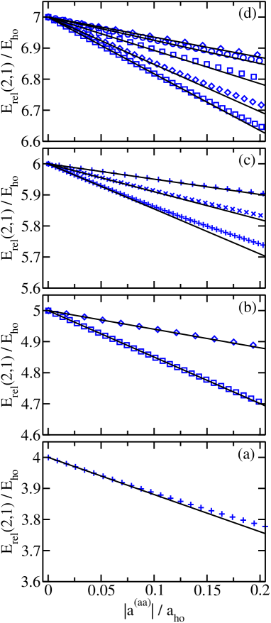
Figure 3: (Color online) Three-fermion energies as a function of the absolute value of the $s$-wave scattering length $|a^{(aa)}|$ for small $|a^{(aa)}|$, $a^{(aa)}\leq 0$, and (a) $E_{\mathrm{rel}}(2,1)\approx 4\hbar\omega$, (b) $E_{\mathrm{rel}}(2,1)\approx 5\hbar\omega$, (c) $E_{\mathrm{rel}}(2,1)\approx 6\hbar\omega$, and (d) $E_{\mathrm{rel}}(2,1)\approx 7\hbar\omega$. Squares, pluses, diamonds, crosses and circles show the essentially exact zero-range energies obtained by solving Eq. (33) for $L_{\mathrm{rel}}=0-4$. For comparison, solid lines show the perturbative results for natural parity states. The solid lines correspond to (a) $(L_{\mathrm{rel}},\Pi_{\mathrm{rel}})=(1,-1)$; and from bottom to top to (b) $(L_{\mathrm{rel}},\Pi_{\mathrm{rel}})=(0,+1)$ and $(2,+1)$; (c) $(L_{\mathrm{rel}},\Pi_{\mathrm{rel}})=(1,-1)$, $(3,-1)$, and $(1,-1)$; and (d) $(L_{\mathrm{rel}},\Pi_{\mathrm{rel}})=(0,+1)$, $(2,+1)$, $(0,+1)$, $(4,+1)$, and $(2,+1)$.

three-body energy spectrum as a function of $|a^{(aa)}|/a_{\mathrm{ho}}$ for the energies around the first four energy families with $E_{\mathrm{rel}}(2,1)\approx 4\hbar\omega$ to $E_{\mathrm{rel}}(2,1)\approx 7\hbar\omega$. As in Fig. 2, the exact energies are shown by symbols while the perturbative energies corresponding to natural parity states are shown by solid lines. As expected, the perturbative treatment reproduces the exact energies extremely well for small $|a^{(aa)}|/a_{\mathrm{ho}}$ and provides a semi-quantitatively correct description up to $|a^{(aa)}|\approx 0.5a_{\mathrm{ho}}$ (see also Fig. 2, which shows the perturbative energies up to $a_{\mathrm{ho}}/|a^{(aa)}|=2$ or $|a^{(aa)}|=0.5a_{\mathrm{ho}}$).

Table 4 shows that the coefficients $c^{(1)}$ cover a wide range of values. Within each energy family, the state shifted most strongly by the interactions is a natural parity state with the smallest allowed angular momentum $L_{\mathrm{rel}}$. To illustrate the increasing density of states and the spread of the energy levels around the non-interacting degenerate energy manifold, Figs. 4(a) and (b) show the frequency with which the

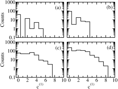
Figure 4: Frequency of the coefficients $c^{(1)}$, which characterize the energy shifts $E^{(1)}$ of the weakly-interacting atomic Fermi gas, for the three- and four-fermion systems. Panels (a) and (b) show the distribution of the $c^{(1)}$ coefficients for $E_{\mathrm{rel}}(2,1)\approx 7\hbar\omega$ (fourth energy manifold of the three-fermion system) and for $E_{\mathrm{rel}}(2,1)\approx 8\hbar\omega$ (fifth energy manifold of the three-fermion system). Panels (c) and (d) show the distribution of the $c^{(1)}$ coefficients for $E_{\mathrm{rel}}(2,2)\approx 19\hbar\omega/2$ (fourth energy manifold of the four-fermion system) and for $E_{\mathrm{rel}}(2,2)\approx 21\hbar\omega/2$ (fifth energy manifold of the four-fermion system). Note the log scale of the vertical axis.

coefficients $c^{(1)}$ occur for $E_{\mathrm{rel}}(2,1)\approx 7\hbar\omega$ (fourth energy manifold) and $E_{\mathrm{rel}}(2,1)\approx 8\hbar\omega$ (fifth energy manifold), respectively. In making this plot, the $2L_{\mathrm{rel}}+1$ degeneracy of the energy levels has been taken into account. Since the unnatural parity states are not affected by the zero-range interactions, the distribution of the $c^{(1)}$ coefficients shows a large amplitude for the $c^{(1)}=0$ bin. Figures 4(a) and (b) show that the spread of the coefficients $c^{(1)}$ increases slightly as the energy manifold increases. The primary characteristic of the distributions of the $c^{(1)}$ coefficients is, however, that the amplitude increases with increasing energy.

We now consider the weakly-repulsive regime, i.e., the regime where $a^{(aa)}/a_{\mathrm{ho}}\ll 1$ and $a^{(aa)}>0$. In this regime, Fig. 2 shows two families of energy levels: (i) energy levels with positive energy and (ii) energy levels with negative energy. The positive energy branches correspond to states that describe a gas of atoms; we refer to these states as the “gas-like state” family. The energies of this family are, in the $a^{(aa)}\rightarrow 0^{+}$ limit, well described by treating the atomic Fermi gas perturbatively (see solid lines in Fig. 2). The negative energy branches correspond to states that can be thought of as consisting of a bound diatomic molecule and a spare atom; we refer to these states as “dimer plus atom” family. In agreement with the literature (see, e.g., Ref. petr03 ), Fig. 2 shows that the formation of bound triatomic molecules is prohibited by the Pauli exclusion principle or the so-called Pauli pressure. For small and positive $a^{(aa)}$, the perturbative energy shifts for the energy levels with $L_{\mathrm{rel}}=0$ and $\Pi_{\mathrm{rel}}=+1$ [dashed lines in Fig. 2(a)] are calculated using Eq. (II.1) with $k=ad$. The perturbative approach, applied to the effective model Hamiltonian $H^{\mathrm{eff}}$, predicts no energy shift for states with $L_{\mathrm{rel}}>0$. This follows directly from the fact that we parametrized the effective atom-dimer interaction through a zero-range $s$-wave potential. Thus, the “bending” of the dashed lines in Fig. 2(b) for $L_{\mathrm{rel}}=1$ (and in general, $L_{\mathrm{rel}}>0$) and positive $a^{(aa)}$ is solely due to the internal energy of the dimer and not due to the effective atom-dimer interaction. We find that the perturbative treatment provides a qualitatively correct description up to $a^{(aa)}\approx 0.5a_{\mathrm{ho}}$.

The effective model Hamiltonian $H^{\mathrm{eff}}$ also provides an intuitive picture for why the lowest $L_{\mathrm{rel}}=0$ state has a lower energy than the lowest $L_{\mathrm{rel}}=1$ state as $a^{(aa)}\rightarrow 0^{+}$. In the $a^{(aa)}\rightarrow 0^{+}$ limit, the diatomic molecule has vanishing angular momentum and the angular momentum $L_{\mathrm{rel}}$ must be carried by the atom-dimer distance vector. Thus, the energy of the lowest state with $L_{\mathrm{rel}}=1$ lies approximately $\hbar\omega$ above the lowest state with $L_{\mathrm{rel}}=0$, the energy of the lowest state with $L_{\mathrm{rel}}=2$ lies approximately $\hbar\omega$ above the lowest state with $L_{\mathrm{rel}}=1$, and so on. The parity inversion of the energetically lowest lying state ($L_{\mathrm{rel}}=1$ and $\Pi_{\mathrm{rel}}=-1$ in the $a^{(aa)}\rightarrow 0^{-}$ limit, and $L_{\mathrm{rel}}=0$ and $\Pi_{\mathrm{rel}}=+1$ in the $a^{(aa)}\rightarrow 0^{+}$ limit) occurs at $a_{\mathrm{ho}}/a^{(aa)}\approx 1$ and has already been pointed out by a number of works kest07 ; stet07 ; stec08 .

Motivated by the fact that the energy spectrum of the three-fermion system can be described by an effective atom plus dimer model in the $a^{(aa)}\rightarrow 0^{+}$ limit, symbols in Figs. 5(a)-(d) show the quantity $E_{\mathrm{rel}}(2,1)-E_{\mathrm{dimer}}$ as a function of the inverse atom-atom scattering length $1/a^{(aa)}$ for $L_{\mathrm{rel}}=0-3$.

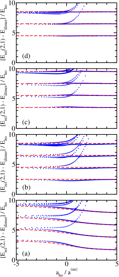
Figure 5: (Color online) Symbols show the scaled energies $E_{\mathrm{rel}}(2,1)-E_{\mathrm{dimer}}$ as a function of the inverse scattering length $a_{\mathrm{ho}}/a^{(aa)}$ for (a) $(L_{\mathrm{rel}},\Pi_{\mathrm{rel}})=(0,+1)$, (b) $(L_{\mathrm{rel}},\Pi_{\mathrm{rel}})=(1,-1)$, (c) $(L_{\mathrm{rel}},\Pi_{\mathrm{rel}})=(2,+1)$, and (d) $(L_{\mathrm{rel}},\Pi_{\mathrm{rel}})=(3,-1)$. For comparison, dashed lines show the energies predicted by the effective atom-dimer model, which provides a semi-quantitative description of the states belonging to the “atom plus dimer” family (see text for details).

Here, $E_{\mathrm{dimer}}$ denotes the lowest eigenenergy of the trapped $s$-wave interacting atom-atom system, i.e., the lowest eigenenergy of Eq. (15) with $k=aa$. The quantity $E_{\mathrm{rel}}(2,1)-E_{\mathrm{dimer}}$ has been investigated previously kest07 ; stec08 and has been termed the universal energy crossover curve in Ref. stec08 . Figures 5(b)-(d) show the existence of a family of states for $L_{\mathrm{rel}}>0$ whose scaled energies are nearly independent of the $s$-wave scattering length $a^{(aa)}$. These scaled energies are approximately given by $(2n_{\mathrm{eff}}+L_{\mathrm{rel}}+3/2)\hbar\omega$ [see dashed lines in Figs. 5(b)-(d)]. The fairly good agreement between the symbols and the dashed lines reflects the fact that a subset of the three-fermion energies can be described to a fairly good approximation by treating the three-fermion system as consisting of a bound trapped $s$-wave dimer plus a non-interacting spare atom. Figures 5(b)-(d) show that this effective dimer-atom description improves with increasing $L_{\mathrm{rel}}$.

The fact that a subset of states of the three-particle spectrum is reasonably well described by the effective dimer plus atom model suggests that the three-particle energy spectrum can be described in terms of avoided crossings between “atom plus dimer” states and “gas-like” states. An interpretation along this line has been quantified by von Stecher stec08d who applied a diabatization scheme. Here, we do not follow the diabatization scheme but instead offer a qualitative discussion of the natural parity three-fermion spectrum with $L_{\mathrm{rel}}>0$. We make four observations: (i) A sequence of states has an energy $E_{\mathrm{rel}}(2,1)$ of approximately $(2+L_{\mathrm{rel}}+2n)\hbar\omega$ at unitarity, an energy $E_{\mathrm{rel}}(2,1)$ of approximately $(3+L_{\mathrm{rel}}+2n)\hbar\omega$ in the $a^{(aa)}\rightarrow 0^{-}$ limit, and an energy $E_{\mathrm{rel}}(2,1)$ of approximately $E_{\mathrm{dimer}}+(3/2+L_{\mathrm{rel}}+2n)\hbar\omega$ in the $a^{(aa)}\rightarrow 0^{+}$ limit [see Fig. 2(b); the states discussed here are those with approximately constant $E_{\mathrm{rel}}(2,1)-E_{\mathrm{dimer}}$, see Figs. 5(b)-(d)]. (ii) For each $L_{\mathrm{rel}}$, the degeneracy of the energy families with $E_{\mathrm{ni,rel}}=(3+L_{\mathrm{rel}}+2n)\hbar\omega$, $n=0,1,\cdots$, increases by one (or $2L_{\mathrm{rel}}+1$ if the degeneracy of the different $M_{L}$ values is accounted for explicitly) as $n$ increases by one (see Fig. 2, Fig. 5 and Table 4). (iii) The energy spectrum corresponding to “gas-like” states has to be identical in the limits $a^{(aa)}\rightarrow 0^{-}$ and $a^{(aa)}\rightarrow 0^{+}$. (iv) It can be easily checked that (i)-(iii) are consistent with the fact that the energy $E_{\mathrm{rel}}(2,1)$ of all but one level of each non-interacting manifold with a given $L_{\mathrm{rel}}$ decreases by $\hbar\omega$ when going from $a^{(aa)}\rightarrow 0^{-}$ to $a^{(aa)}\rightarrow\infty$ and by another $\hbar\omega$ when going from $a^{(aa)}\rightarrow\infty$ to $a^{(aa)}\rightarrow 0^{+}$. The dropping of the energies by $2\hbar\omega$ as $a^{(aa)}$ changes from $0^{-}$ through $\pm\infty$ to $0^{+}$ is similar to the $2\hbar\omega$ dropping of the excited state $s$-wave energies of the two-particle system (see dashed lines in Fig. 1) and can be interpreted as one pair (consisting of a spin-up atom and a spin-down atom) feeling the $s$-wave interaction while the other spin-up atom carrying the angular momentum.

Interestingly, the observations described in the previous paragraph allow for an approximate determination of the $K_{\mathrm{unit}}$ coefficients [see Eq. (32)]. Observation (i) implies that the lowest $K_{\mathrm{unit}}$ coefficient for a given $L_{\mathrm{rel}}$ is approximately given by $K_{\mathrm{unit,model}}=L_{\mathrm{rel}}+1/2$ in the large $L_{\mathrm{rel}}$ limit. As discussed in Sec. II.2, each $K_{\mathrm{unit}}$ coefficient determines the starting point of a ladder of energy levels, which are spaced by $2\hbar\omega$ and which are associated with an increasing number of nodes along the hyperradial coordinate $R$. It is evident from Figs. 5(b)-(d) that these states, which are characterized by the same hyperangular quantum number but different hyperradial quantum numbers $q$, transform into atom plus dimer states in the $a^{(aa)}\rightarrow 0^{+}$ limit, which are characterized by the effective orbital angular momentum quantum number $l_{\mathrm{eff}}=0$ and different radial quantum numbers $n_{\mathrm{eff}}$. Interpreting the atom-dimer distance coordinate as the hyperradial coordinate in the $a^{(aa)}\rightarrow 0^{+}$ limit, the identification $q\leftrightarrow n_{\mathrm{eff}}$ suggests itself. Using observation (iv), the remaining $K_{\mathrm{unit}}$ coefficients at unitarity are approximately given by $K_{\mathrm{unit,model}}=L_{\mathrm{rel}}+1/2+2n$ for $L_{\mathrm{rel}}>0$ and natural parity states [for each $n=1,2,\cdots$, the $q$ quantum number in Eq. (32) takes the values $q=0,1,\cdots$]. Figure 6(a) shows

Figure 6: (Color online) Symbols show the coefficients $K_{\mathrm{unit}}$ that correspond to natural parity states for (a) the three-fermion system and (b) the four-fermion system as a function of the angular momentum quantum number $L_{\mathrm{rel}}$. Dotted lines show the coefficients $K_{\mathrm{unit,model}}$ (see text for details).

that the difference between $K_{\mathrm{unit}}$ (symbols) and $K_{\mathrm{unit,model}}$ (dotted lines) decreases as $L_{\mathrm{rel}}$ increases. The difference between $K_{\mathrm{unit}}$ and $K_{\mathrm{unit,model}}$ has previously been quantified by Werner and Castin within a semi-classical WKB framework wern06a .

The $L_{\mathrm{rel}}=0$ spectrum is different from the $L_{\mathrm{rel}}>0$ spectra for two reasons. First, the effective atom-dimer system is described by an effective atom-dimer $s$-wave scattering length $a^{(ad)}$, which leads to a decrease of approximately $\hbar\omega$ of the energy levels belonging to the atom plus dimer family as $a^{(aa)}$ changes from $\infty$ to $0^{+}$. Second, the symmetry constraint in the $a^{(aa)}\rightarrow 0^{-}$ limit pushes the energy of the lowest $L_{\mathrm{rel}}=0$ state up by $\hbar\omega$ compared to that with $L_{\mathrm{rel}}=1$. Dashed lines in Fig. 5(a) show the eigenenergies of the effective atom plus dimer model, i.e., the eigenenergies of Eq. (15) for $k=ad$ with $a^{(ad)}$ given by Eq. (13). It can be seen that the agreement between the energies of this effective model and a subset of the full three-fermion energies is good for small positive $a^{(aa)}$ and qualitatively correct throughout the entire crossover regime. Using the effective atom plus dimer model, the energy at unitarity of a subset of states is approximately given by $E_{\mathrm{rel}}(2,1)\approx E_{\mathrm{dimer}}+(2q+5/2)\hbar\omega$, implying $K_{\mathrm{unit,model}}=3/2$. For comparison, the exact value is $K_{\mathrm{unit}}=1.666$ wern06a . The other $K_{\mathrm{unit}}$ coefficients for $L_{\mathrm{rel}}=0$ can be estimated by using that the energy of one subset of states drops by $\hbar\omega$ in going from $a^{(aa)}\rightarrow\infty$ to $a^{(aa)}\rightarrow 0^{+}$, implying $E_{\mathrm{unit,rel}}(2,1)\approx(5/2+2q+2n)\hbar\omega$ with $n=1,2,\cdots$ and $q=0,1,\cdots$. This estimate yields $K_{\mathrm{unit,model}}=5/2+2n$ for $n=1,2,\cdots$. Figure 6(a) shows that the $K_{\mathrm{unit,model}}$ (dotted lines) reproduce the exact $K_{\mathrm{unit}}$ coefficients (symbols) fairly well.

III.2 Four-fermion system

This section discusses the energy spectrum of the four-fermion system throughout the BCS-BEC crossover. We primarily focus on the energies corresponding to natural parity states but also consider those corresponding to unnatural states. To determine the energy spectrum corresponding to states with natural parity, we use the stochastic variational approach with the basis functions given in Eq. (36); our basis set optimization either treats one state at a time or a subset of states simultaneously. For a given atom-atom scattering length $a^{(aa)}$, we determine the energies for various ranges $r_{0}$, $r_{0}=0.01a_{\mathrm{ho}}-0.09a_{\mathrm{ho}}$, of the two-body Gaussian interaction potential and extrapolate the finite-range energies to $r_{0}\rightarrow 0$. For negative scattering lengths $a^{(aa)}$, we find that the four-fermion energies depend linearly on $r_{0}$ for all $L_{\mathrm{rel}}$ considered. In this regime, we typically calculate the energies for three different $r_{0}$ and then determine the $r_{0}\rightarrow 0$ energies by performing a linear fit. For positive scattering lengths $a^{(aa)}$, the energetically low-lying part of the spectrum is dominated by the “internal” energy of the dimer(s) formed. As discussed in more detail below, the lowest energy family for even $L_{\mathrm{rel}}$ can be described by an effective two-boson model while the lowest energy family for odd $L_{\mathrm{rel}}$ consists of states that can be thought of as consisting of a dimer and two atoms as $a^{(aa)}\rightarrow 0^{+}$ (see Sec. II and below). Correspondingly, for positive $a^{(aa)}$ and even $L_{\mathrm{rel}}$, we subtract twice the dimer binding energy from the four-fermion energies for each $r_{0}$ and extrapolate the scaled four-fermion energies to the $r_{0}\rightarrow 0$ limit. We typically consider five different $r_{0}$ and extract the scaled zero-range energies by performing a quadratic fit to the scaled finite-range four-fermion energies. The zero-range four-fermion energies themselves are then obtained by adding twice the zero-range dimer energy, i.e., $2E_{\mathrm{dimer}}$. For odd $L_{\mathrm{rel}}$, we subtract (and later add) the dimer energy as opposed to twice the dimer energy but proceed analogously otherwise.

The energies of a large number of energy levels corresponding to natural parity states are reported in the auxiliary materials epaps for atom-atom scattering lengths $a^{(aa)}$ ranging from $0^{-}$ over $\infty$ to $0.2a_{\mathrm{ho}}$ for $L_{\mathrm{rel}}\leq 4$. To the best of our knowledge, these are the first comprehensive benchmark results for the four-fermion system with finite angular momentum throughout the crossover region. Tables 6

Table 6: Extrapolated zero-range energies $E_{\mathrm{unit,rel}}(2,2)$ for natural parity states with $L_{\mathrm{rel}}\leq 4$ [$E_{\mathrm{unit,rel}}(2,2)\leq 8.5\hbar\omega$]. The uncertainty of the energies is estimated to be in the last digit reported. For comparison, the lowest energy of the $(L_{\mathrm{rel}},\Pi_{\mathrm{rel}})=(1,+1)$ state is $E_{\mathrm{unit,rel}}=5.088(20)\hbar\omega$.

$L_{\mathrm{rel}}$	$\Pi_{\mathrm{rel}}$	$q$	$K_{\mathrm{unit}}$	$E_{\mathrm{unit,rel}}/E_{\mathrm{ho}}$
0	$+1$	0	2.009	3.509
0	$+1$	1	2.010	5.510
0	$+1$	0	4.444	5.944
0	$+1$	0	5.029	6.529
0	$+1$	0	5.347	6.847
0	$+1$	2	2.017	7.517
0	$+1$	1	4.446	7.946
0	$+1$	0	6.864	8.364
0	$+1$	0	6.905	8.405
1	$-1$	0	4.098	5.598
1	$-1$	0	4.176	5.676
1	$-1$	0	4.730	6.230
1	$-1$	0	5.669	7.169
1	$-1$	0	5.807	7.307
1	$-1$	1	4.101	7.601
1	$-1$	1	4.180	7.680
1	$-1$	0	6.505	8.005
1	$-1$	0	6.724	8.224
1	$-1$	1	4.732	8.232
1	$-1$	0	6.904	8.404
2	$+1$	0	2.918	4.418
2	$+1$	0	4.539	6.039
2	$+1$	1	2.920	6.420
2	$+1$	0	5.039	6.539
2	$+1$	0	5.629	7.129
2	$+1$	0	5.722	7.222
2	$+1$	0	5.925	7.425
2	$+1$	0	5.927	7.427
2	$+1$	1	4.542	8.042
2	$+1$	0	6.707	8.207
2	$+1$	2	2.924	8.424
2	$+1$	0	7.001	8.501
3	$-1$	0	4.676	6.176
3	$-1$	0	5.871	7.371
3	$-1$	0	6.191	7.691
3	$-1$	0	6.194	7.694
3	$-1$	1	4.678	8.178
3	$-1$	0	6.764	8.264
3	$-1$	0	6.771	8.271
3	$-1$	0	6.904	8.404
3	$-1$	0	6.977	8.477
4	$+1$	0	4.985	6.485
4	$+1$	0	5.838	7.338
4	$+1$	0	5.868	7.368
4	$+1$	0	6.865	8.365
4	$+1$	1	4.984	8.484

and 7

Table 7: Lowest two extrapolated zero-range energies $E_{\mathrm{unit,rel}}(2,2)$ for the four-fermion system with natural parity and $L_{\mathrm{rel}}=5-8$ at unitarity. The uncertainty of the extrapolated zero-range energies is estimated to be in the last or second last digit reported.

$L_{\mathrm{rel}}$	$\Pi_{\mathrm{rel}}$	$q$	$K_{\mathrm{unit}}$	$E_{\mathrm{unit,rel}}/E_{\mathrm{ho}}$
5	$-1$	0	6.745	8.245
5	$-1$	0	6.790	8.290
6	$+1$	0	6.996	8.496
6	$+1$	0	7.781	9.281
7	$-1$	0	8.769	10.269
7	$-1$	0	8.777	10.277
8	$+1$	0	8.998	10.498
8	$+1$	0	9.775	11.275

summarize the energies of the four-fermion system at unitarity for natural parity states with $L_{\mathrm{rel}}=0$ to $L_{\mathrm{rel}}=8$ as well as for one unnatural parity state. For $L_{\mathrm{rel}}>0$, these are the first results at unitarity. We estimate that our extrapolated zero-range energies for the energetically lowest-lying $L_{\mathrm{rel}}=0$ state is accurate to better than 0.1% for most scattering lengths $a^{(aa)}$, including infinitely large $a^{(aa)}$. Near the avoided crossings around $a^{(aa)}\approx a_{\mathrm{ho}}$ (see, e.g., Fig. 10), however, the accuracy decreases by up to an order of magnitude. Generally speaking, we find that the accuracy of the extrapolated zero-range energies also decreases for energetically higher lying states and for states with larger $L_{\mathrm{rel}}$. The eigenenergies reported in Tables 6 and 7 are labeled by the hyperradial quantum number $q$. Following Eq. (32), we identify this quantum number by looking for $2\hbar\omega$ spacings between energy pairs. Inspection of Table 6 shows that the energies with $q>0$ lie, within our numerical accuracy, $2\hbar\omega$ above an energy with $q-1$ (see the nearly identical $K_{\mathrm{unit}}$ coefficients in the fourth column of Tables 6 and 7). Figure 6(b) shows the $K_{\mathrm{unit}}$ coefficients corresponding to natural parity states of the four-fermion system as a function of $L_{\mathrm{rel}}$. Compared to the three-fermion system, the four-fermion system exhibits a notably denser energy spectrum at unitarity [see Fig. 6(a) and 6(b)].

Lines in Fig. 7 show the extrapolated zero-range energies for the four-fermion system

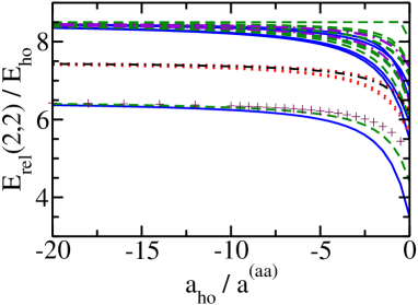
Figure 7: (Color online) Four-fermion energies $E_{\mathrm{rel}}(2,2)$ as a function of the inverse $s$-wave scattering length $a_{\mathrm{ho}}/a^{(aa)}$ with $1/a^{(aa)}\leq 0$. For $a^{(aa)}\rightarrow 0^{-}$, all energy levels corresponding to natural parity states around $E_{\mathrm{ni,rel}}=13\hbar\omega/2$, $15\hbar\omega/2$ and $17\hbar\omega/2$ are shown. Solid, dotted, dashed, dash-dotted and dash-dash-dotted lines show the zero-range energies corresponding to natural parity states with $L_{\mathrm{rel}}=0$ to $L_{\mathrm{rel}}=4$. Pluses show the energy of the energetically lowest-lying unnatural parity state with $L_{\mathrm{rel}}=1$.

corresponding to natural parity states with $L_{\mathrm{rel}}=0$ to $L_{\mathrm{rel}}=4$ as a function of the inverse $s$-wave scattering length $1/a^{(aa)}$ for negative $a^{(aa)}$. In the $a^{(aa)}\rightarrow 0^{-}$ limit, the three energetically lowest-lying four-fermion energy manifolds around $E_{\mathrm{ni,rel}}(2,2)=13\hbar\omega/2$, $15\hbar\omega/2$ and $17\hbar\omega/2$ consist of two, four and 15 states, respectively (here, the $2L_{\mathrm{rel}}+1$ degeneracy due to the $M_{L}$ quantum number is not included in counting the states; see also Table 5). For comparison, pluses in Fig. 7 show the energetically lowest lying unnatural parity state with ($L_{\mathrm{rel}},\Pi_{\mathrm{rel}})=(1,+1)$; in this case, the energies are calculated for a Gaussian two-body potential with small but finite $r_{0}$ and have not been extrapolated to the $r_{0}\rightarrow 0$ limit. Figure 7 shows that the three energy manifolds remain distinguishable up to $a_{\mathrm{ho}}/a^{(aa)}\approx-2$ but start to overlap notably in the strongly-interacting regime.

We now discuss the weakly-attractive regime of the four-fermion energy spectrum in more detail. The coefficients $c^{(1)}$ that determine the perturbative energy shifts $E^{(1)}$ are summarized in the last column of Table 5 for the first three energy manifolds with $E_{\mathrm{ni,rel}}=13\hbar\omega/2$, $15\hbar\omega/2$ and $17\hbar\omega/2$. Figure 8

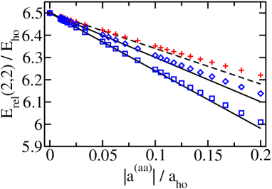
Figure 8: (Color online) Four-fermion energies $E_{\mathrm{rel}}(2,2)$ as a function of the absolute value of the $s$-wave scattering length $|a^{(aa)}|$ for small $|a^{(aa)}|$, $a^{(aa)}\leq 0$, and $E_{\mathrm{rel}}(2,2)\approx 13\hbar\omega/2$. Squares, diamond and pluses show the numerically determined four-fermion energies for $(L_{\mathrm{rel}},\Pi_{\mathrm{rel}})=(0,+1)$, $(L_{\mathrm{rel}},\Pi_{\mathrm{rel}})=(2,+1)$ and $(L_{\mathrm{rel}},\Pi_{\mathrm{rel}})=(1,+1)$, respectively. Solid and dashed lines show the perturbative results for natural and unnatural parity states, respectively.

compares the four-fermion spectrum near $E_{\mathrm{rel}}(2,2)\approx 13/2\hbar\omega$ calculated by the stochastic variational approach [squares, diamonds and pluses show the energy levels corresponding to states with $(L_{\mathrm{rel}},\Pi_{\mathrm{rel}})=(0,+1)$, $(2,+1)$ and $(1,+1)$, respectively] with that calculated perturbatively (solid and dashed lines show the energies corresponding to states with natural and unnatural parity, respectively). As expected, the agreement is excellent for small $|a^{(aa)}|$ and worsens with increasing $|a^{(aa)}|$. For small $|a^{(aa)}|$, the energy level with unnatural parity is affected less strongly by the two-body interactions than the energy levels with natural parity. Inspection of Table 5 shows that this is a general trend, i.e., within a given manifold the energy level shifted most strongly is that corresponding to the natural parity state with the smallest allowed angular momentum.

To illustrate the behavior of the energy spectrum for a higher energy manifold, Fig. 9 shows the energies corresponding to the eight states with $(L_{\mathrm{rel}},\Pi_{\mathrm{rel}})=(2,+1)$

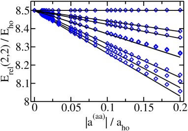
Figure 9: (Color online) Four-fermion energies $E_{\mathrm{rel}}(2,2)$ as a function of the absolute value of the $s$-wave scattering length $|a^{(aa)}|$ for small $|a^{(aa)}|$ ($a^{(aa)}\leq 0$), $E_{\mathrm{rel}}(2,2)\approx 17\hbar\omega/2$ and $(L_{\mathrm{rel}},\Pi_{\mathrm{rel}})=(2,+1)$. Diamonds show the numerically determined four-fermion energies while solid lines show the perturbative results. Note that the fourth and fifth state (counted from the bottom) are nearly degenerate for the scattering length range depicted.

around $E_{\mathrm{rel}}\approx 17\hbar\omega/2$. Again, the agreement between the numerically determined energies (diamonds) and the perturbatively determined energies (solid lines) is excellent for small $|a^{(aa)}|$. Interestingly, within the perturbative treatment, one of the $(L_{\mathrm{rel}},\Pi_{\mathrm{rel}})=(2,+1)$ states is not affected by the $s$-wave interactions, implying that the wave function vanishes whenever two unlike fermions approach each other closely. It turns out that the perturbative result in this case is exact, i.e., there exists a $(L_{\mathrm{rel}},\Pi_{\mathrm{rel}})=(2,+1)$ state with energy $E_{\mathrm{rel}}(2,2)=17\hbar\omega/2$ for all scattering lengths $a^{(aa)}$.

Figures 4(c) and (d) show the distributions of the $c^{(1)}$ coefficients for the fourth and fifth energy manifolds with $E_{\mathrm{rel}}(2,2)\approx 19\hbar\omega/2$ and $E_{\mathrm{rel}}(2,2)\approx 21\hbar\omega/2$, respectively. Compared to the three-particle case [Figs. 4(a) and (b)], the degeneracies increase more rapidly as can be seen by the higher frequency with which the $c^{(1)}$ coefficients occur. Furthermore, the $c^{(1)}=0$ bin no longer dominates the distribution since both natural and unnatural parity states are effected by the zero-range interactions.

Next, we discuss the energy spectrum in the strongly-interacting regime and in the $a^{(aa)}\rightarrow 0^{+}$ limit. For small $a^{(aa)}$, the energetically lowest lying states with even $L_{\mathrm{rel}}$ belong to the “dimer plus dimer” family while the energetically lowest lying states with odd $L_{\mathrm{rel}}$ belong to the “dimer plus atom plus atom” family. Motivated by this observation (see also Refs. stec07c ; stec08 ; stec08d ) and by our discussion of the three-fermion system (see Sec. III.1), Figs. 10(a), (b) and (c)

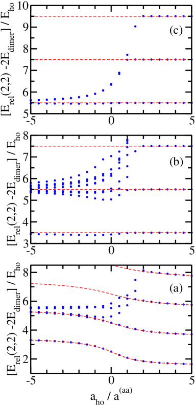
Figure 10: (Color online) Scaled four-fermion energies $E_{\mathrm{rel}}(2,2)-2E_{\mathrm{dimer}}$ as a function of $a_{\mathrm{ho}}/a^{(aa)}$ for (a) $(L_{\mathrm{rel}},\Pi_{\mathrm{rel}})=(0,+1)$, (b) $(L_{\mathrm{rel}},\Pi_{\mathrm{rel}})=(2,+1)$ and (c) $(L_{\mathrm{rel}},\Pi_{\mathrm{rel}})=(4,+1)$. Symbols show the numerically determined energies while dashed lines show the energies predicted by the effective dimer-dimer model (see text for details).

show the scaled energies $E_{\mathrm{rel}}(2,2)-2E_{\mathrm{dimer}}$ for $L_{\mathrm{rel}}=0,2$ and 4. The scaled four-fermion spectra for $L_{\mathrm{rel}}=2$ and 4 contain a set of nearly constant scaled energies given by $E_{\mathrm{rel}}(2,2)-2E_{\mathrm{dimer}}\approx(3/2+L_{\mathrm{rel}}+2q)\hbar\omega$, where $q=0,1,\cdots$ [see dashed lines in Figs. 10(b) and (c)]. Figures 10(b) and (c) show that this description improves with increasing $L_{\mathrm{rel}}$. The set of constant scaled energies $E_{\mathrm{rel}}(2,2)-2E_{\mathrm{dimer}}$ is predicted to exist within the effective two-boson model, which treats the composite bosons as non-interacting if $L_{\mathrm{rel}}>0$ and $L_{\mathrm{rel}}$ even [see the discussion below Eq. (15) in Sec. II]. Using that a subset of the scaled energies is approximately constant and that the dimer energy $E_{\mathrm{dimer}}$ equals $\hbar\omega/2$ at unitarity, the lowest $K_{\mathrm{unit}}$ coefficient is, for $L_{\mathrm{rel}}$ even and $L_{\mathrm{rel}}>0$, approximately given by $K_{\mathrm{unit,model}}=L_{\mathrm{rel}}+1$. The energy levels associated with these $K_{\mathrm{unit}}$ coefficients have the minimally allowed number of excitations in the hyperangular degrees of freedom and $q$ excitations along the hyperradial coordinate $R$; these states transform, as $a^{(aa)}$ changes from $\infty$ to $0^{+}$, to “dimer plus dimer” states with $n_{\mathrm{eff}}$ radial excitations. Since the dimers are composite bosons, an analogous set of states does not exist for odd $L_{\mathrm{rel}}$. Squares in Fig. 11 show the difference between

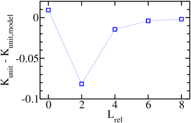
Figure 11: (Color online) Symbols show the difference between the lowest coefficient $K_{\mathrm{unit}}$ obtained from our numerically determined four-fermion energies and the lowest coefficient $K_{\mathrm{unit,model}}$ predicted by the simple dimer-dimer model discussed in the text as a function of $L_{\mathrm{rel}}$ ($L_{\mathrm{rel}}$ even). To guide the eye symbols are connected by dotted lines.

the lowest $K_{\mathrm{unit}}$ coefficient and $K_{\mathrm{unit,model}}$, where $K_{\mathrm{unit}}$ is taken from Tables 6 and 7 for $L_{\mathrm{rel}}=2-8$ and $L_{\mathrm{rel}}$ even. This figure supports our conjecture that the lowest coefficient $K_{\mathrm{unit}}$ converges to the value $K_{\mathrm{unit,model}}$ in the large $L_{\mathrm{rel}}$ limit.

The behavior of the scaled energies for $L_{\mathrm{rel}}=0$ is different from that of the scaled energies for $L_{\mathrm{rel}}>0$ ($L_{\mathrm{rel}}$ even). Figure 10(a) does not show a set of nearly constant scaled energy levels but instead shows a set of scaled energies that drop by approximately $\hbar\omega$ in going from $a^{(aa)}\rightarrow 0^{-}$ to $a^{(aa)}=\infty$ and by another $\hbar\omega$ in going from $a^{(aa)}=\infty$ to $a^{(aa)}\rightarrow 0^{+}$. Dashed lines in Fig. 10 show the energies predicted by the effective dimer-dimer model. To obtain these energies, we solve Eq. (15) for $k=dd$ and use Eq. (14) to express the effective dimer-dimer scattering length $a^{(dd)}$ in terms of the atom-atom scattering length $a^{(aa)}$ throughout the entire crossover. The dashed lines agree surprisingly well with the full four-fermion energies throughout the entire crossover. Comparison with Fig. 5(a) shows that the effective two-particle model provides a better description of the four-fermion than of the three-fermion system, particularly for negative $a^{(aa)}$. Intuitively, this might be explained by the fact that the three-fermion system contains an unpaired atom while all atoms participate in the molecule formation in the four-fermion system. Figure 10 suggests that the four-fermion energy spectrum can be interpreted by considering avoided crossings between dimer-dimer states and states that belong to the “dimer plus atom plus atom” and the “gas-like state” families. An analysis along these lines has been performed in Refs. stec07c ; stec08d ; however, to the best of our knowledge this type of analysis has not been previously applied to estimate the value of the lowest $K_{\mathrm{unit}}$ coefficient for $L_{\mathrm{rel}}=0$. Using that the energy in the $a^{(aa)}\rightarrow 0^{+}$ limit is given by $2E_{\mathrm{dimer}}+(3/2+2n_{\mathrm{eff}})\hbar\omega$ and that the energy at unitarity is—using the argument above—$2E_{\mathrm{dimer}}+(5/2+2q)\hbar\omega$, the lowest $K_{\mathrm{unit}}$ coefficient for $L_{\mathrm{rel}}=0$ can be estimated to be $K_{\mathrm{unit,model}}=2$. Table 6 shows that this model is surprisingly accurate, i.e., $K_{\mathrm{unit}}=2.009$ (see also Fig. 11).

We find numerically that the second lowest $K_{\mathrm{unit}}$ coefficient for even $L_{\mathrm{rel}}$ ($\Pi_{\mathrm{rel}}=+1$) and the lowest $K_{\mathrm{unit}}$ coefficient for odd $L_{\mathrm{rel}}$ ($\Pi_{\mathrm{rel}}=-1$) appear to approach $L_{\mathrm{rel}}+7/4$ for large $L_{\mathrm{rel}}$. At present, we have no explanation for this observation. While our analysis presented above allows for the prediction of the lowest $K_{\mathrm{unit}}$ coefficient for all even $L_{\mathrm{rel}}$, the remaining coefficients at unitarity appear to be result of an intricate interplay of how to best distribute the angular momentum among the six interparticle distances.

IV Summary

This paper considered $s$-wave interacting three- and four-fermion systems under external spherically symmetric harmonic confinement. If the range $r_{0}$ of the underlying interaction potential is much smaller than the other length scales of the system, i.e., the atom-atom $s$-wave scattering length $a^{(aa)}$ and the harmonic oscillator length $a_{\mathrm{ho}}$, then the physics of two-component equal-mass Fermi systems is universal. If the $s$-wave scattering length is tuned in the vicinity of a so-called broad Feshbach resonance dien04 ; petr05 ; gior08 , then the low-energy properties of these few-fermion systems are expected to behave universally, i.e., independently of the details of the underlying interaction potential. Our results are expected to apply to the experimentally most frequently studied species ⁶Li and ⁴⁰K dema99 ; grei03 ; zwie03 ; bour03 ; stre03 ; kina04 ; stew06 .

We have determined the zero-range energy spectrum of the three- and four-fermion systems numerically for a wide range of $s$-wave scattering lengths $a^{(aa)}$. Our study of the three-fermion system is based on the Lippmann-Schwinger equation, which reduces the problem to solving a set of coupled equations for each angular momentum $L_{\mathrm{rel}}$ kest07 . The three-fermion spectrum is analyzed and interpreted following a number of different approaches. In the weakly-interacting regime, the interactions are treated as a perturbation to the non-interacting trapped atomic Fermi gas. This approach correctly describes the gas-like states of the system for small $|a^{(aa)}|$, with $a^{(aa)}$ positive and negative, but does not describe states that are associated with the formation of diatomic molecules. The energies of this family of states are described by an effective two-particle Hamiltonian that treats the diatomic molecule as a composite point particle and assumes that the spare atom and the molecule interact through the $s$-wave scattering channel characterized by the effective atom-dimer scattering length $a^{(ad)}$. Somewhat surprisingly, this effective two-particle model describes the energies of a subset of states not only quantitatively correctly in the weakly-repulsive regime but also qualitatively for negative $a^{(aa)}$ (see dashed lines in Fig. 5). Building on this observation, we developed a simple model which predicts the $K_{\mathrm{unit}}$ coefficients with reasonably good accuracy. In doing so, our motivation was to develop a physical picture of the general features of the three-fermion energy spectrum that can, at least partially, be generalized to larger systems. A key result of our analysis is that the energy levels determined by the lowest $K_{\mathrm{unit}}$ coefficient for each $L_{\mathrm{rel}}$ transform to “atom plus dimer” states as $a^{(aa)}$ changes from $\infty$ to $0^{+}$. This “transformation” of the states can be interpreted nicely within the hyperspherical framework. Using hyperspherical coordinates, the states for $a^{(aa)}=\infty$ and $0^{+}$ are separable and the widths of the avoided crossings of the energy levels for finite $a^{(aa)}$ are determined by the couplings between different hyperradial potential curves (see, e.g., Refs. delv58 ; delv60 ; mace68 ; lin95 as well as Ref. stec08d ).

We also solved the time-independent Schrödinger equation for the four-fermion system for a Gaussian two-body potential with varying range $r_{0}$ using the stochastic variational approch. The resulting finite-range energies were then extrapolated to the $r_{0}\rightarrow 0$ limit. The energy spectrum of the four-fermion system is much denser than that of the three-fermion system. Unlike for the three-fermion system, natural and unnatural parity states of the four-fermion system are shifted by the zero-range interactions. Our primary focus in this paper has been to characterize the energies of the lowest few states with natural parity throughout the crossover, including the infinitely strongly-interacting unitary regime. As in the three-fermion case, our semi-analytical perturbative approach, which utilizes hyperspherical coordinates, reproduces the numerically determined four-fermion energies with good accuracy in the weakly-attractive and weakly-repulsive regimes. We paid special attention to the infinitely strongly-interacting regime and analyzed the energy spectrum at unitarity within an effective two-boson model. This analysis provides a physical picture of how the lowest $K_{\mathrm{unit}}$ coefficient for natural parity states and even $L_{\mathrm{rel}}$ comes about and how the associated ladder of states transforms to “dimer plus dimer” states as $a^{(aa)}\rightarrow 0^{+}$. Furthermore, the fact that the effective two-boson model reproduces a subset of energy levels semi-quantitatively throughout the entire crossover regime suggests that the concept of the effective dimer-dimer scattering length $a^{(dd)}$ extends beyond the small $a^{(aa)}$ regime ($a^{(aa)}>0$).

One motivation for studying small few-fermion systems is to develop a “bottom-up approach” that investigates the microscopic physics of two-component Fermi gases by treating successively larger systems. With this motivation in mind, the three-fermion system can be considered the smallest system that models spin-imbalanced Fermi gases kest07 while the four-fermion system can be considered the smallest system that models pairing physics throughout the BCS-BEC crossover of spin-balanced Fermi gases stec07c . In the future, it will be interesting to extend the studies presented here to larger equal-mass few-fermion systems as well as to unequal-mass fermionic and bosonic systems. We also hope to use the perturbative treatment of the four-fermion system to estimate the fourth order virial coefficient in the weakly-interacting regimes.

Support by the NSF through grant PHY-0855332 and by the ARO are gratefully acknowledged.

Auxiliary material for “Energy spectrum of harmonically trapped two-component Fermi gases: Three- and Four-Particle Problem”

This EPAPS material contains the extrapolated zero-range energies $E_{\mathrm{rel}}(2,2)$ for negative scattering lengths $a^{(aa)}$, and the extrapolated scaled zero-range energies $E_{\mathrm{rel}}(2,2)-2E_{\mathrm{dimer}}$ and $E_{\mathrm{rel}}(2,2)-E_{\mathrm{dimer}}$ for positive scattering lengths $a^{(aa)}$. The notation follows that of the main article.

Table 8: Energies $E_{\mathrm{rel}}(2,2)$ for various $L_{\mathrm{rel}}$ and $a^{(aa)}$. The energies (second through 8th column) are reported in units of $E_{\mathrm{ho}}$. Columns two through six show the energies for the five lowest states with $(L_{\mathrm{rel}},\Pi_{\mathrm{rel}})=(0,+1)$ while columns seven through nine show the energies for the three lowest states with $(L_{\mathrm{rel}},\Pi_{\mathrm{rel}})=(1,-1)$. The uncertainty of the energies is estimated to be in the second to last digit for large $|a^{(aa)}|$ and 1 in the last digit reported for small $|a^{(aa)}|$. “NI” stands for non-interacting ($a^{(aa)}=0$).

$a_{\mathrm{ho}}/a^{(aa)}$			$L_{\mathrm{rel}}=0$				$L_{\mathrm{rel}}=1$
NI	$13/2$	$17/2$	$17/2$	$17/2$	$17/2$	$15/2$	$15/2$	$15/2$
$-100$	6.4741	8.4704	8.4721	8.4850	8.4885	7.4801	7.4824	7.4887
$-90$	6.4712	8.4671	8.4691	8.4834	8.4872	7.4779	7.4804	7.4875
$-80$	6.4676	8.4630	8.4652	8.4813	8.4856	7.4751	7.4780	7.4859
$-70$	6.4630	8.4577	8.4602	8.4787	8.4835	7.4716	7.4748	7.4840
$-60$	6.4569	8.4507	8.4536	8.4751	8.4808	7.4669	7.4707	7.4813
$-50$	6.4482	8.4409	8.4444	8.4701	8.4770	7.4603	7.4648	7.4775
$-40$	6.4354	8.4261	8.4306	8.4627	8.4712	7.4505	7.4561	7.4720
$-30$	6.4139	8.4016	8.4076	8.4503	8.4617	7.4342	7.4416	7.4627
$-20$	6.3714	8.3528	8.3620	8.4257	8.4427	7.4019	7.4127	7.4443
$-18$	6.3572	8.3366	8.3469	8.4176	8.4364	7.3913	7.4032	7.4382
$-16$	6.3397	8.3164	8.3281	8.4074	8.4285	7.3780	7.3913	7.4306
$-14$	6.3172	8.2906	8.3041	8.3944	8.4184	7.3611	7.3761	7.4208
$-12$	6.2873	8.2564	8.2723	8.3771	8.4050	7.3388	7.3560	7.4080
$-10$	6.2460	8.2090	8.2283	8.3532	8.3863	7.3080	7.3282	7.3901
$-19/2$	6.2330	8.1931	8.2136	8.3455	8.3801	7.2983	7.3195	7.3846
$-9$	6.2187	8.1766	8.1984	8.3372	8.3736	7.2877	7.3099	7.3784
$-17/2$	6.2027	8.1583	8.1815	8.3280	8.3663	7.2759	7.2992	7.3715
$-8$	6.1848	8.1379	8.1626	8.3177	8.3581	7.2628	7.2873	7.3638
$-15/2$	6.1647	8.1149	8.1414	8.3060	8.3488	7.2480	7.2738	7.3552
$-7$	6.1419	8.0889	8.1174	8.2928	8.3382	7.2313	7.2586	7.3454
$-13/2$	6.1158	8.0592	8.0900	8.2778	8.3261	7.2123	7.2412	7.3342
$-6$	6.0857	8.0250	8.0584	8.2604	8.3119	7.1904	7.2213	7.3212
$-11/2$	6.0506	7.9853	8.0218	8.2401	8.2953	7.1650	7.1980	7.3062
$-5$	6.0091	7.9386	7.9788	8.2161	8.2755	7.1353	7.1706	7.2884
$-9/2$	5.9594	7.8830	7.9276	8.1875	8.2514	7.0998	7.1379	7.2671
$-4$	5.8989	7.8159	7.8658	8.1528	8.2216	7.0571	7.0983	7.2413
$-7/2$	5.8238	7.7337	7.7899	8.1097	8.1837	7.0046	7.0495	7.2092
$-3$	5.7284	7.6308	7.6948	8.0553	8.1342	6.9389	6.9879	7.1687
$-5/2$	5.6040	7.4994	7.5732	7.9845	8.0667	6.8544	6.9085	7.1158
$-2$	5.4361	7.3270	7.4133	7.8899	7.9700	6.7432	6.8027	7.0448
$-3/2$	5.2009	7.0936	7.1990	7.7588	7.8230	6.5916	6.6573	6.9456
$-1$	4.8569	6.7641	6.9062	7.5698	7.5847	6.3779	6.4497	6.8009
$-1/2$	4.3324	6.2745	6.5041	7.1829	7.2863	6.0663	6.1426	6.5796
$0$	3.5092	5.5101	5.9441	6.5290	6.8482	5.5978	5.6758	6.2305

Table 9: Nine lowest energies $E_{\mathrm{rel}}(2,2)$ for $(L_{\mathrm{rel}},\Pi_{\mathrm{rel}})=(2,+1)$ and various $a^{(aa)}$. The energies (second through 10th column) are reported in units of $E_{\mathrm{ho}}$. The uncertainty of the energies is estimated to be in the second to last digit for large $|a^{(aa)}|$ and 1 in the last digit reported for small $|a^{(aa)}|$.

$a_{\mathrm{ho}}/a^{(aa)}$					$L_{\mathrm{rel}}=2$
NI	13/2	17/2	17/2	17/2	17/2	17/2	17/2	17/2	17/2
$-100$	6.4801	8.4766	8.4789	8.4816	8.4872	8.4872	8.4924	8.4942	8.5001
$-90$	6.4779	8.4740	8.4765	8.4796	8.4858	8.4858	8.4915	8.4936	8.5001
$-80$	6.4751	8.4706	8.4735	8.4769	8.4838	8.4838	8.4903	8.4927	8.5001
$-70$	6.4716	8.4665	8.4698	8.4737	8.4817	8.4817	8.4891	8.4917	8.5001
$-60$	6.4669	8.4610	8.4648	8.4694	8.4787	8.4787	8.4873	8.4903	8.5001
$-50$	6.4604	8.4532	8.4579	8.4633	8.4745	8.4745	8.4847	8.4884	8.5001
$-40$	6.4506	8.4416	8.4474	8.4541	8.4681	8.4682	8.4809	8.4855	8.5002
$-30$	6.4344	8.4223	8.4300	8.4388	8.4576	8.4578	8.4746	8.4807	8.5002
$-20$	6.4023	8.3841	8.3957	8.4085	8.4367	8.4372	8.4619	8.4711	8.5003
$-18$	6.3918	8.3714	8.3843	8.3984	8.4298	8.4304	8.4577	8.4679	8.5003
$-16$	6.3786	8.3556	8.3703	8.3858	8.4213	8.4220	8.4524	8.4639	8.5004
$-14$	6.3619	8.3354	8.3522	8.3697	8.4104	8.4112	8.4457	8.4588	8.5004
$-12$	6.3398	8.3087	8.3285	8.3484	8.3959	8.3970	8.4367	8.4520	8.5005
$-10$	6.3094	8.2717	8.2956	8.3187	8.3760	8.3774	8.4243	8.4425	8.5005
$-19/2$	6.2992	8.2579	8.2841	8.3079	8.3695	8.3712	8.4205	8.4394	8.5012
$-9$	6.2887	8.2450	8.2728	8.2976	8.3626	8.3645	8.4161	8.4361	8.5013
$-17/2$	6.2771	8.2306	8.2602	8.2861	8.3550	8.3570	8.4113	8.4324	8.5013
$-8$	6.2642	8.2145	8.2462	8.2732	8.3464	8.3487	8.4058	8.4283	8.5014
$-15/2$	6.2494	8.1964	8.2304	8.2587	8.3368	8.3393	8.3997	8.4235	8.5014
$-7$	6.2329	8.1759	8.2127	8.2422	8.3260	8.3287	8.3927	8.4182	8.5015
$-13/2$	6.2141	8.1525	8.1924	8.2234	8.3136	8.3166	8.3848	8.4120	8.5016
$-6$	6.1925	8.1254	8.1692	8.2018	8.2994	8.3028	8.3755	8.4049	8.5016
$-11/2$	6.1675	8.0939	8.1423	8.1765	8.2828	8.2867	8.3646	8.3965	8.5017
$-5$	6.1380	8.0566	8.1109	8.1467	8.2634	8.2678	8.3518	8.3864	8.5018
$-9/2$	6.1030	8.0121	8.0735	8.1112	8.2402	8.2453	8.3362	8.3743	8.5020
$-4$	6.0607	7.9581	8.0287	8.0680	8.2122	8.2181	8.3172	8.3593	8.5021
$-7/2$	6.0087	7.8911	7.9738	8.0147	8.1777	8.1847	8.2933	8.3402	8.5022
$-3$	5.9432	7.8064	7.9053	7.9475	8.1343	8.1428	8.2627	8.3155	8.5024
$-5/2$	5.8587	7.6964	7.8178	7.8606	8.0782	8.0888	8.2219	8.2819	8.5025
$-2$	5.7459	7.5496	7.7027	7.7451	8.0035	8.0170	8.1658	8.2342	8.5028
$-3/2$	5.5895	7.3473	7.5456	7.5865	7.9001	7.9180	8.0847	8.1620	8.5030
$-1$	5.3613	7.0597	7.3211	7.3615	7.7501	7.7757	7.9610	8.0430	8.5033
$-1/2$	5.0077	6.6422	6.9799	7.0320	7.5194	7.5610	7.7613	7.8277	8.5036
$0$	4.4185	6.0390	6.4201	6.5391	7.1288	7.2218	7.4247	7.4271	8.0416

Table 10: Energies $E_{\mathrm{rel}}(2,2)$ for various $L_{\mathrm{rel}}$ and $a^{(aa)}$. The energies (second through 5th column) are reported in units of $E_{\mathrm{ho}}$. Column two shows the energy for the lowest state with $(L_{\mathrm{rel}},\Pi_{\mathrm{rel}})=(3,-1)$ while columns three through five show the energies for the three lowest states with $(L_{\mathrm{rel}},\Pi_{\mathrm{rel}})=(4,+1)$. The uncertainty of the energies is estimated to be in the second to last digit for large $|a^{(aa)}|$ and 1 in the last digit reported for small $|a^{(aa)}|$.

$a_{\mathrm{ho}}/a^{(aa)}$	$L_{\mathrm{rel}}=3$		$L_{\mathrm{rel}}=4$
NI	15/2	17/2	17/2	17/2
$-100$	7.4861	8.4823	8.4901	8.4908
$-90$	7.4845	8.4804	8.4890	8.4898
$-80$	7.4826	8.4778	8.4874	8.4884
$-70$	7.4802	8.4748	8.4858	8.4869
$-60$	7.4769	8.4706	8.4835	8.4847
$-50$	7.4723	8.4648	8.4802	8.4817
$-40$	7.4655	8.4561	8.4753	8.4771
$-30$	7.4541	8.4416	8.4671	8.4695
$-20$	7.4318	8.4130	8.4509	8.4544
$-18$	7.4244	8.4036	8.4456	8.4494
$-16$	7.4153	8.3918	8.4389	8.4432
$-14$	7.4036	8.3769	8.4304	8.4352
$-12$	7.3882	8.3571	8.4192	8.4247
$-10$	7.3671	8.3298	8.4036	8.4100
$-19/2$	7.3602	8.3206	8.3987	8.4053
$-9$	7.3529	8.3112	8.3933	8.4002
$-17/2$	7.3449	8.3007	8.3873	8.3945
$-8$	7.3359	8.2890	8.3807	8.3881
$-15/2$	7.3258	8.2759	8.3732	8.3810
$-7$	7.3144	8.2610	8.3646	8.3728
$-13/2$	7.3014	8.2440	8.3549	8.3636
$-6$	7.2865	8.2245	8.3437	8.3529
$-11/2$	7.2693	8.2018	8.3307	8.3403
$-5$	7.2490	8.1751	8.3153	8.3255
$-9/2$	7.2250	8.1432	8.2969	8.3077
$-4$	7.1961	8.1046	8.2745	8.2860
$-7/2$	7.1606	8.0569	8.2469	8.2588
$-3$	7.1162	7.9965	8.2119	8.2242
$-5/2$	7.0593	7.9179	8.1662	8.1786
$-2$	6.9841	7.8121	8.1046	8.1163
$-3/2$	6.8812	7.6630	8.0182	8.0275
$-1$	6.7346	7.4409	7.8909	7.8944
$-1/2$	6.5164	7.0871	7.6837	7.6926
$0$	6.1756	6.4855	7.3384	7.3677

Table 11: Scaled energies $E_{\mathrm{rel}}(2,2)-2E_{\mathrm{dimer}}$ for various $L_{\mathrm{rel}}$ and $a^{(aa)}$. The scaled energies (second to 10th column) are reported in units of $E_{\mathrm{ho}}$. Columns two through four show the scaled energies for the three lowest states with $(L_{\mathrm{rel}},\Pi_{\mathrm{rel}})=(0,+1)$, columns five through seven show the scaled energies for the three lowest states with $(L_{\mathrm{rel}},\Pi_{\mathrm{rel}})=(2,+1)$ and columns eight through ten show the scaled energies for the three lowest states with $(L_{\mathrm{rel}},\Pi_{\mathrm{rel}})=(4,+1)$. The uncertainty of the scaled energies is estimated to be in the last digit reported.

$a_{\mathrm{ho}}/a^{(aa)}$		$L_{\mathrm{rel}}=0$			$L_{\mathrm{rel}}=2$			$L_{\mathrm{rel}}=4$
$1/2$	2.281	4.357	5.190	3.457	5.239	5.539	5.495	6.836	6.890
$1$	2.082	4.206	5.718	3.486	5.464	6.073	5.499	7.493	7.719
$3/2$	1.939	4.072	6.138	3.497	5.486	7.264	5.500	7.503	9.033
$2$	1.843	3.967	6.045	3.499	5.496	7.500	5.500	7.501	9.508
$5/2$	1.778	3.888	5.963	3.501	5.499	7.504	5.500	7.501	9.506
$3$	1.732	3.831	5.899	3.500	5.500	7.506	5.500	7.501	9.504
$7/2$	1.699	3.787	5.848	3.501	5.500	7.503	5.500	7.501	9.504
$4$	1.673	3.752	5.807	3.502	5.500	7.502	5.500	7.501	9.501
$9/2$	1.653	3.724	5.773	3.501	5.500	7.502	5.500	7.501	9.501
$5$	1.637	3.701	5.745	3.500	5.500	7.502	5.500	7.501	9.501

Table 12: Scaled energies $E_{\mathrm{rel}}(2,2)-E_{\mathrm{dimer}}$ for various $L_{\mathrm{rel}}$ and $a^{(aa)}$. The scaled energies (second through 5th column) are reported in units of $E_{\mathrm{ho}}$. Columns two through four show the scaled energies for the three lowest states with $(L_{\mathrm{rel}},\Pi_{\mathrm{rel}})=(1,-1)$ and column five shows the scaled energy for the lowest state with $(L_{\mathrm{rel}},\Pi_{\mathrm{rel}})=(3,-1)$. The uncertainty of the scaled energies is estimated to be in the last digit reported.

$a_{\mathrm{ho}}/a^{(aa)}$		$L_{\mathrm{rel}}=1$		$L_{\mathrm{rel}}=3$
$1/2$	4.927	4.999	5.703	5.667
$1$	4.774	4.834	5.708	5.697
$3/2$	4.654	4.699	5.745	5.753
$2$	4.562	4.593	5.795	5.813
$5/2$	4.490	4.511	5.841	5.863
$3$	4.433	4.446	5.880	5.900
$7/2$	4.387	4.395	5.909	5.926
$4$	4.350	4.352	5.931	5.945
$9/2$	4.318	4.318	5.947	5.958
$5$	4.289	4.290	5.959	5.968

References

- (1) L. Platter, H. W. Hammer, and U. G. Meissner, Phys. Rev. A 70, 052101 (2004).
- (2) M. T. Yamashita, L. Tomio, A. Delfino, and T. Frederico, Europhys. Lett. 75, 555 (2006).
- (3) G. J. Hanna and D. Blume, Phys. Rev. A 74, 063604 (2006).
- (4) H. W. Hammer and L. Platter, Eur. Phys. J. A 32, 113 (2007).
- (5) J. von Stecher, J. P. D’Incao, and C. H. Greene, Nature Phys. 5, 417 (2009).
- (6) Y. J. Wang and B. D. Esry, Phys. Rev. Lett. 102, 133201 (2009).
- (7) F. Ferlaino, S. Knoop, M. Berninger, W. Harm, J. P. D’Incao, H.-C. Nägerl, and R. Grimm, Phys. Rev. Lett. 102, 140401 (2009).
- (8) M. Zaccanti, B. Deissler, C. D’Errico, M. Fattori, M. Jona-Lasinio, S. Müller, G. Roati, M. Inguscio, and G. Modugno, Nature Phys. 5, 586 (2009).
- (9) S. E. Pollack, D. Dries, and R. G. Hulet, Science 326, 1683 (2009).
- (10) E. Braaten and H.-W. Hammer, Phys. Rep. 428, 259 (2006).
- (11) G. A. Baker, Jr., Phys. Rev. C 60, 054311 (1999).
- (12) K. M. O’Hara, S. L. Hemmer, M. E. Gehm, S. R. Granade, and J. E. Thomas, Science 298, 2179 (2002).
- (13) T.-L. Ho, Phys. Rev. Lett. 92, 090402 (2004).
- (14) S. Tan, cond-mat/0412764v2 (2004).
- (15) S. Y. Chang and V. R. Pandharipande, Phys. Rev. Lett. 95, 080402 (2005).
- (16) G. E. Astrakharchik, J. Boronat, J. D. Casulleras, and S. Giorgini, Phys. Rev. Lett. 93, 200404 (2004).
- (17) S. Y. Chang, V. R. Pandharipande, J. Carlson, and K. E. Schmidt, Phys. Rev. A 70, 043602 (2004).
- (18) J. E. Thomas, J. Kinast, and A. Turlapov, Phys. Rev. Lett. 95, 120402 (2005).
- (19) Y. Castin, C. R. Phys. 5, 407 (2004).
- (20) F. Werner and Y. Castin, Phys. Rev. A 74, 053604 (2006).
- (21) D. T. Son and M. Wingate, Ann. Phys. 321, 197 (2006).
- (22) J. T. Stewart, J. P. Gaebler, C. A. Regal, and D. S. Jin, Phys. Rev. Lett. 97, 220406 (2006).
- (23) S. Tan, Ann. Phys. 323, 2952 (2008).
- (24) S. Tan, Ann. Phys. 323, 2971 (2008).
- (25) S. Tan, Ann. Phys. 323, 2987 (2008).
- (26) E. Braaten and L. Platter, Phys. Rev. Lett. 100, 205301 (2008).
- (27) E. Braaten, D. Kang, and L. Platter, Phys. Rev. A 78, 053606 (2008).
- (28) F. Werner and Y. Castin, cond-mat/1001.0774 (2010).
- (29) M. Greiner, O. Mandel, T. Esslinger, T. W. Hänsch, and I. Bloch, Nature 415, 39 (2002).
- (30) M. Köhl, H. Moritz, T. Stöferle, K. Günter, and T. Esslinger, Phys. Rev. Lett. 94, 080403 (2005).
- (31) G. Thalhammer, K. Winkler, F. Lang, S. Schmid, R. Grimm, and J. Hecker Denschlag, Phys. Rev. Lett. 96, 050402 (2006).
- (32) F. Werner and Y. Castin, Phys. Rev. Lett. 97, 150401 (2006).
- (33) J. P. Kestner and L. M. Duan, Phys. Rev. A 76, 033611 (2007).
- (34) I. Stetcu, B. R. Barrett, U. van Kolck, and J. P. Vary, Phys. Rev. A 76, 063613 (2007).
- (35) J. von Stecher, C. H. Greene, and D. Blume, Phys. Rev. A 77, 043619 (2008).
- (36) K. Varga and Y. Suzuki, Phys. Rev. C 52, 2885 (1995).
- (37) K. Varga, P. Navratil, J. Usukura, and Y. Suzuki, Phys. Rev. B 63, 205308 (2001).
- (38) Y. Suzuki and K. Varga, Stochastic Variational Approach to Quantum Mechanical Few-Body Problems (Springer Verlag, Berlin, 1998).
- (39) H. H. B. Sørensen, D. V. Fedorov, and A. S. Jensen, Nuclei and Mesoscopic Physics, ed. by V. Zelevinsky, AIP Conf. Proc. No. 777 (AIP, Melville, NY, 2005), p. 12.
- (40) J. von Stecher and C. H. Greene, Phys. Rev. Lett. 99, 090402 (2007).
- (41) J. von Stecher, C. H. Greene, and D. Blume, Phys. Rev. A 76, 053613 (2007).
- (42) D. Blume, J. von Stecher, and C. H. Greene, Phys. Rev. Lett. 99, 233201 (2007).
- (43) D. Blume and K. M. Daily, Phys. Rev. A 80, 053626 (2009).
- (44) J. Avery, Hyperspherical Harmonics: Applications in Quantum Theory (Kluwer Academic Publishers, Dordrecht, Boston, London, 1989).
- (45) C. D. Lin, Phys. Rep. 257, 1 (1995).
- (46) J. L. Bohn, B. D. Esry, and C. H. Greene, Phys. Rev. A 58, 584 (1998).
- (47) N. K. Timofeyuk, Phys. Rev. C 65, 064306 (2002).
- (48) N. K. Timofeyuk, Phys. Rev. C 69, 034336 (2004).
- (49) M. F. de la Ripelle, S. A. Sofianos, and R. M. Adam, Ann. Phys. 316, 107 (2005).
- (50) S. T. Rittenhouse, M. J. Cavagnero, J. von Stecher, and C. H. Greene, Phys. Rev. A 74, 053624 (2006).
- (51) U. Fano, D. Green, J. L. Bohn, and T. A. Heim, J. Phys. B 32, R1 (1999).
- (52) S. T. Rittenhouse and C. H. Greene, J. Phys. B 41, 205302 (2008).
- (53) E. Fermi, Nuovo Cimento 11, 157 (1934).
- (54) D. S. Petrov, C. Salomon, and G. V. Shlyapnikov, Phys. Rev. Lett. 93, 090404 (2004).
- (55) D. S. Petrov, C. Salomon, and G. V. Shlyapnikov, J. Phys. B 38, S645 (2005).
- (56) D. S. Petrov, Phys. Rev. A 67, 010703(R) (2003).
- (57) K. Huang and C. N. Yang, Phys. Rev. 105, 767 (1957).
- (58) G. V. Skorniakov and K. A. Ter-Martirosian, Zh. Eksp. Teor. Fiz. 31, 775 (1956) [Sov. Phys. JETP 4, 648 (1957)].
- (59) C. Mora, R. Egger, A. O. Gogolin, and A. Komnik, Phys. Rev. Lett. 93, 170403 (2004).
- (60) C. Mora, R. Egger, and A. O. Gogolin, Phys. Rev. A 71, 052705 (2005).
- (61) T. Busch, B.-G. Englert, K. Rza̧żewski, and M. Wilkens, Foundations of Phys. 28, 549 (1998).
- (62) V. Efimov, Yad. Fiz. 12, 1080 (1970) [Sov. J. Nucl. Phys. 12, 598 (1971)].
- (63) V. N. Efimov, Nucl. Phys. A 210, 157 (1973).
- (64) J. P. D’Incao and B. D. Esry, Phys. Rev. Lett. 94, 213201 (2005).
- (65) J. von Stecher and C. H. Greene, Phys. Rev. A 80, 022504 (2009).
- (66) X.-J. Liu, H. Hu, and P. D. Drummond, Phys. Rev. Lett. 102, 160401 (2009).
- (67) J. von Stecher, Ph. D. thesis (2008), University of Colorado, Boulder; available at http://jila.colorado.edu/pubs/thesis/.
- (68) See EPAPS Document No. XXX for auxiliary material (four-body energies). For more information on EPAPS, see .
- (69) S. Giorgini, L. P. Pitaevskii, and S. Stringari, Rev. Mod. Phys. 80, 1215 (2008).
- (70) R. B. Diener and T.-L. Ho, arXiv:cond-mat/0405174.
- (71) B. DeMarco and D. S. Jin, Science 285, 1703 (1999).
- (72) M. Greiner, C. A. Regal, and D. S. Jin, Nature 426, 537 (2003).
- (73) M. W. Zwierlein, C. A. Stan, C. H. Schunck, S. M. F. Raupach, S. Gupta, Z. Hadzibabic, and W. Ketterle, Phys. Rev. Lett. 91, 250401 (2003).
- (74) T. Bourdel, J. Cubizolles, L. Khaykovich, K. M. F. Magalhaes, S. J. J. M. F. Kokkelmans, G. V. Shlyapnikov, and C. Salomon, Phys. Rev. Lett. 91, 020402 (2003).
- (75) K. E. Strecker, G. B. Partridge, and R. G. Hulet, Phys. Rev. Lett. 91, 080406 (2003).
- (76) J. Kinast, S. L. Hemmer, M. E. Gehm, A. Turlapov, and J. E. Thomas, Phys. Rev. Lett. 92, 150402 (2004).
- (77) L. M. Delves, Nucl. Phys. 9, 391 (1958).
- (78) L. M. Delves, Nucl. Phys. 20, 275 (1960).
- (79) J. Macek, J. Phys. B 1, 831 (1968).