The evolution of cloud cores and the formation of stars

Abstract

For a number of starless cores, self-absorbed molecular line and column density observations have implied the presence of large-amplitude oscillations. We examine the consequences of these oscillations on the evolution of the cores and the interpretation of their observations. We find that the pulsation energy helps support the cores and that the dissipation of this energy can lead toward instability and star formation. In this picture, the core lifetimes are limited by the pulsation decay timescales, dominated by non-linear mode-mode coupling, and on the order of $\simeq{\rm few}\times 10^{5}$–$10^{6}\,{\rm yr}$. Notably, this is similar to what is required to explain the relatively low rate of conversion of cores into stars. For cores with large-amplitude oscillations, dust continuum observations may appear asymmetric or irregular. As a consequence, some of the cores that would be classified as supercritical may be dynamically stable when oscillations are taken into account. Thus, our investigation motivates a simple hydrodynamic picture, capable of reproducing many of the features of the progenitors of stars without the inclusion of additional physical processes, such as large-scale magnetic fields.

1 Introduction

The starless cores owe their reputation as the sites of future star formation to the similarities they share with neighboring cores already in the pains of stellar birth. Small (tenths of pc), dense ($n_{\rm H_{2}}\sim 10^{3}$ to $10^{6}$ cm^-3) dark clouds of a few solar masses, the starless cores contain no infrared sources above the sensitivity level of the IRAS satellite (about 0.1 L_⊙ at the distance of Taurus). Mixed in with a population of cores, embedded infrared protostars, and young T-Tauri stars, the starless cores seem on the verge of issue. (Myers et al. 1983; Myers & Benson 1983; Benson & Myers 1989; Beichman et al. 1986; di Francesco et al. 2007; Ward-Thompson et al. 2007; Bergin & Tafalla 2007).

The starless cores are remarkable in another sense. They may be the only structures in the interstellar medium in quasi-static equilibrium with lifetimes longer than their sound-crossing times (Beichman et al. 1986; Jessop & Ward-Thompson 2000; Kirk et al. 2005; Ward-Thompson et al. 2007). Whereas all larger-scale clouds are better described as transient structures within a turbulent cascade (Field et al. 2008), the starless cores show observed densities that are consistently matched (Ward-Thompson et al. 1994; Andre et al. 1996; Ward-Thompson et al. 1999; Bacmann et al. 2000; Evans et al. 2001; Alves et al. 2001; Tafalla et al. 2002; Kandori et al. 2005; Kirk et al. 2005) by the truncated solutions of the isothermal Lane-Emden equation, i.e., the Bonnor-Ebert (BE) spheres (Bonnor 1956). These are self-gravitating spheres supported by thermal energy and bounded by an external pressure. The source of the external pressure appears to depend upon the star forming region, though its necessity is well documented. Within the Pipe nebula, the core energetics are consistent with a constant external pressure supplied by hotter, more rareified gas (Lada et al. 2008). In other regions, such as Lupus (Teixeira et al. 2005), the cores appear to be surrounded by lower density molecular gas with observed molecular line widths $\geq 1$ kms. Here and in similar regions small-scale (smaller than the observing beam) supersonic turbulence in the low-density molecular gas around the cores may supply the confining pressure.

While a continuous extension to the larger-scale ISM prompts the question of whether the cores are individual dynamical entities, a distinct boundary is evident in several observations. First, maps of dust absorption in the Taurus region (Bacmann et al. 2000) often show sharp edges defining the core boundaries. Second, around at least one core, B5, a boundary is defined by a sharp transition (within less than an observing beam width) between subsonic and supersonic turbulence in the molecular gas (Pineda et al. 2010). Third, a boundary is a necessary feature in models of radiative cooling and UV heating (Evans et al. 2001; Shirley et al. 2002; Zucconi et al. 2001; Stamatellos & Whitworth 2003; Gonçalves et al. 2004; Keto & Field 2005) that use the basic BE structure and accurately predict the observed gas and dust temperatures (Ward-Thompson et al. 2002; Pagani et al. 2003, 2004; Crapsi et al. 2007), the observed variation in the excitation of the CO molecule across the starless cores (Bergin et al. 2006; Schnee et al. 2007; Keto & Caselli 2008), and the observed brightness and profiles of molecular lines (Keto & Caselli 2010).

The predictive success of models based on BE spheres (including a core boundary) implies that the starless cores are indeed individual dynamic entities in quasi-static equilibrium, balancing the forces of their own self-gravity, internal energy, and the larger-scale ISM. In some cases, this equilibrium may be unstable, leading the core to contract, though their internal pressure is sufficiently high to prevent free-fall.

The hydrodynamic equations that describe the equilibrium configuration of both stars and the starless cores allow for perturbations in the form of sonic waves that may persist for many crossing times. Such oscillations are observed in the Sun, other main sequence stars, and white dwarfs, and given the turbulent state of the larger-scale ISM, should be expected in the starless cores as well. Analytic (Keto et al. 2006) and numerical (Keto & Field 2005; Broderick et al. 2007) models of oscillating cores easily reproduce the characteristic asymmetric shapes of molecular lines seen in the starless cores. While the spectral-line profiles of the low-order modes (the dipolar and breathing modes are observational indistinguishable from simple contraction, expansion and rotation) a few cores show simultaneous inward and outward motions (Aguti et al. 2007; Lada et al. 2003; Redman et al. 2006) that are consistent only with oscillatory modes. Oscillations produce density perturbations as well, and the dipole and quadrupole modes naturally reproduce the ellipsoidal morphologies (Keto et al. 2006) characteristically seen in observations of the cores (Bacmann et al. 2000; Ward-Thompson et al. 1999; Kirk et al. 2005).

Observations suggest that these oscillations, rather than a minor perturbation on quasi-static equilibrium, provide a substantial contribution to the dynamical stability and therefore are important in the evolution of the cores toward star formation. First, a significant fraction of starless cores have observed density profiles that can only be matched by a BE sphere if the gas temperature in the model sphere is made considerably higher than is known to be the case in the starless cores (Evans et al. 2001; Kirk et al. 2005; Kandori et al. 2005). Second, the sizes of many of the starless cores imply that they should be unstable to gravitational collapse (Evans et al. 2001; Kandori et al. 2005). However, statistical analyses of the relative numbers of stars and cores in a sample of different star-forming regions imply lifetimes that are several times the relevant free-fall time (Beichman et al. 1986; Jessop & Ward-Thompson 2000; Ward-Thompson et al. 2007). Reconciling these observations require a source of energy within the cores in addition to the thermal energy. Internal oscillations or turbulence are suggested by the observation that the spectral line widths in many cores are larger than the expected thermal width (Dickman & Clemens 1983; Myers & Benson 1983; Lada et al. 2008) implying internal subsonic velocities on spatial scales unresolved in the observing beam.

These observations combined with modelling suggest the following evolution for the starless cores: The cores are formed at the bottom of the supersonic turbulent cascade that dominates the larger-scale ISM (Field et al. 2008), producing cores with a spectrum of masses and internal turbulent energies. Those cores massive enough to be gravitationally unstable immediately begin contraction to form a star, while those with appropriate mass and internal energy become self-supported and self-gravitating. These cores are decoupled from the cascade in the sense that they exist as individual dynamical entities independent of the larger-scale flows (Keto & Field 2005). The internal turbulence inherited from the parent flow, and present when a core forms, is part of its initial dynamical stability but is expected to dissipate over time. Thought of as a spectrum of individual modes of oscillation, the turbulence decays by non-linear mode-mode coupling (collisions between modes) (Broderick et al. 2007) and by transmission through the core boundary into the larger-scale ISM (Broderick et al. 2008). The gradual loss of this internal turbulent energy leads eventually (on time scales of several crossing times) to gravitational instability and star formation.

In this paper we explore the latter half of this evolution. We develop a model for the internal turbulence of the cores and examine its consequences for the evolution toward star formation and for the interpretation of dust continuum observations. Using the fact that the turbulence can be fully described as a collection of oscillating modes, we consider three models for the turbulent energy distribution, a Kolmogorov spectrum, a flat spectrum, and a spectrum dominated by long wave lengths. In Section 2 we compute the effective pressure arising from this turbulence. We find that the breathing modes are destabilizing, but modes with shorter wave lengths generate a supporting pressure. In Section 3, we generate random realizations of turbulent cores and find that a typical stable, oscillating core would appear to be dynamically unstable, if the observations were fit to a static BE model. In Section 4, we follow the evolution of the turbulent spectrum as it decays. We find that the spectrum of the turbulence evolves toward dominance by the longer wave lengths. In conclusion, we find that we can describe the evolution of the cores toward star formation as a purely hydrodynamic phenomenon without the necessity of support by large-scale magnetic fields (though a tangled magnetic field may co-exist in equipartition with the turbulence without substantially changing the findings).

2 The Stability of Pulsating Cores

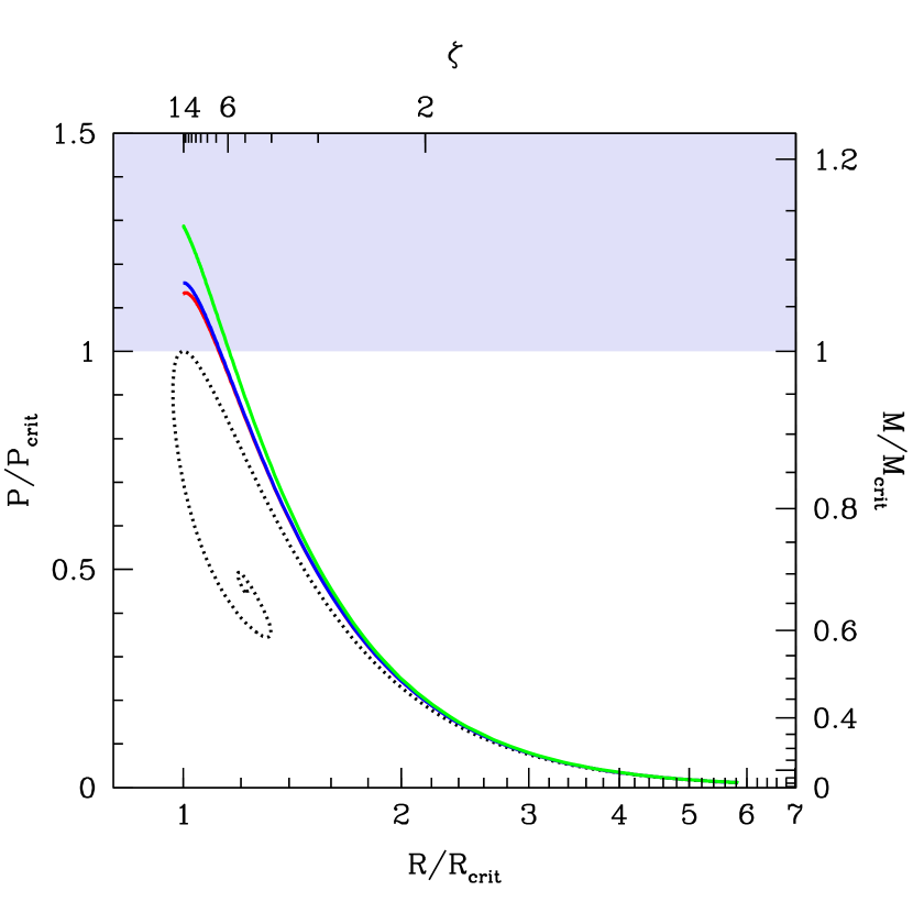
Figure 1: Surface pressure as a function of radius for a pulsating fixed-mass isothermal gas sphere. For reference, the static configuration is shown by the dotted line, and becomes unstable at a center/surface density ratio, $\zeta$, of $14.04$. The red, blue and green lines shown the surface pressure resulting from oscillations containing 30% of the unperturbed configurations gravitational binding energy for the Kolmogorov (Equation 7), Flat (Equation 9) and fundamental-Kolmogorov (Equation 10) energy spectra, respectively. Along the top axis $\zeta$ is shown until the critical value is reached (above which the mapping from $\zeta$ to $R$ is no longer single valued, as evidenced by the spiral structure in $P$ vs. $R$ for $\zeta>\zeta_{\rm crit}$). Along the right axis the corresponding mass at fixed surface pressure is shown. Finally, within the shaded region at the top no stable static configurations exist.

In this section we compute the dynamical consequences of large-scale oscillations for the underlying starless core. We find it is possible for pulsations both to support the core and to initiate collapse, the distinction lying in the relative importance of the low and higher-order oscillation modes. It is possible to do this with a macroscopic description similar to the stability analysis of a BE sphere (Bonnor 1956), requiring only the pulsation frequencies (which depend upon the core structure) and the distribution of energy amongst them. Here we briefly review how stability may be determined by the macroscopic core properties, make explicit the notion of “slow” compression, use this definition to compute the response of the pulsations, and finally assess the consequences for a number of different mode compliments.

2.1 The Stability of Stationary Cores

The starless cores in the BE model are held together by a combination of their own self-gravity and the external pressure, and these two inward forces are resisted by the outward thermal pressure. The dotted line in Figure 1 shows the equilibrium configurations as a function of the external pressure,$P$, and the core size, $R$. At large radii, the portion of the curve to the right of $R/R_{crit}=1$, the gravitational force at the boundary is weak compared to the confining pressure. If we compress a core on this portion of the curve, we find that the internal pressure increases with the increasing density, and a larger external pressure is required to confine the core, $dP/dR<0$. If the compression is removed, the core will re-exand to its original equilibrium. However, if the radius becomes sufficiently small, $R/R_{crit}<1$, gravitational force dominate at the boundary, and a smaller external pressure would be required to maintain equilibrium as the core is compressed, i.e., $dP/dR\geq 0$. In this case, the core can not resist further compression and is therefore unstable to contraction. For static isothermal gas spheres, this is greatly simplified by the fact that the equilibrium configurations form a one-parameter family, which may be chosen such that the relevant parameter is the ratio of the surface and central densities (or, equivalently, pressures), $\zeta$ (Bonnor 1956). In this case the maximum ratio is $\zeta_{crit}=14.04$.

The thought experiment we describe above to define the stability of cores employs a sequence of cores at fixed mass and varying surface pressure. However, it is perhaps more physically appropriate to hold the surface pressure fixed, determined by the properties of the surrounding molecular gas, and vary the core mass instead. That is, at a given surface pressure, core radius and core temperature identify the unique, stable isothermal core mass, $M(R)$ (if an equilibrium configuration exists at all). The mass and pressure are related by the scaling relations that connect gas spheres with identical $\zeta$’s. Explicitly, from the equations of hydrostatic structure, at a given $\zeta$ we have $M\propto c_{s}^{3}/P^{1/2}$, and thus fixing $c_{s}$ (i.e., fixing the core temperature) gives $M\propto P^{-1/2}$. The $P(R)$ shown in Figure 1 are computed at fixed mass, i.e., $M={\rm const}$. Conversely, if we choose $P={\rm const}$, we have

$$\frac{M(R)}{M}=\left[\frac{P(R)}{P}\right]^{1/2}$$ (1)

Thus, the equilibrium core mass $M(R)$ at fixed surface pressure and core temperature is identical, up to a non-linear rescaling, to $P(R)$. In Figure 1 the right-hand vertical axis is labeled with $M(R)$ instead of $P(R)$. Most importantly, $P_{\rm crit}$ corresponds to a critical mass, $M_{\rm crit}$, above which no stable configuration exists.

2.2 Response of Pulsations to Slow Compression

The situation becomes more complicated in the presence of energetically significant pulsations. This is because we must not only adjust the underlying gas configuration, but also the oscillation amplitudes. In principle, a rapid compression can excite oscillations itself, and we must carefully specify the dynamical nature of the experiment we use to define stability. More generally, we must carefully identify how “equilibrium” configurations are defined along the entire $P(R)$ curve. In the static case a similar consideration is already made when we assume that the core mass and temperature are fixed; both are natural physical conditions for the starless cores. Since the core has a boundary, its mass is constant. Radiation provides an efficient thermal coupling to the surrounding medium keeping the core temperature unvarying on a time scale much shorter than the dynamical time scales of the cores (Keto & Caselli 2010).

Although radiative equilibrium violates the adiabatic condition in the strict thermodynamic sense, if the compression is assumed to occur slowly relative to the oscillation periods, we may still treat it as adiabatic for the purposes of evolving the oscillation mode amplitudes. In this case, what remains fixed are the adiabatic invariants of the oscillations. Computing these is simplified by the fact that we may treat the pulsation modes as a collection of uncoupled, one-dimensional harmonic oscillators, with the mode amplitudes defined by the radial and angular quantum numbers $n$, $l$ and $m$ (with their standard definitions), $A_{nlm}$, governed by

$$\frac{d^{2}A_{nlm}}{dt^{2}}=-\omega_{nlm}^{2}A_{nlm}\,,$$ (2)

for a mode dependent angular frequency, $\omega_{nlm}$ (Gingold & Monaghan 1980; Rathore et al. 2003). For this the adiabatic invariant is well known to be $E_{nlm}/\omega_{nlm}$, where $E_{nlm}=M_{nlm}\omega_{nlm}^{2}A_{nlm}^{2}/2$ is the mode energy (in which $M_{nlm}$ is the mode “mass” and computed from the mode structure directly). Thus, we may compute the evolution of the energy in a particular mode during an adiabatic compression, given $\omega_{nlm}(R)$. Specifically, from the adiabatic invariant we obtain

$$\frac{dE_{nlm}}{dR}=\frac{E_{nlm}}{\omega_{nlm}}\frac{d\omega_{nlm}}{dR}\,.$$ (3)

However, the presence of an additional component to the core’s total energy associated with the oscillations, $E_{\rm osc}=\sum_{nlm}E_{nlm}$, also implies the existance of an additional component to the surface pressure. That is, generally, under adiabatic compressions the oscillations will produce a dynamically generated surface pressure

$$P_{\rm osc}\equiv-\frac{dE_{\rm osc}}{dV}=-\frac{d}{dV}\sum_{nlm}E_{nlm}=-\frac{1}{4\pi R^{2}}\sum_{nlm}\frac{E_{nlm}}{\omega_{nlm}}\frac{d\omega_{nlm}}{dR}\,.$$ (4)

Thus, the pulsation contribution to the surface pressure is dependent upon $d\omega_{nlm}/dR$ and the oscillation energy spectrum (which we shall discuss in more detail below).

In the dicussion thus far, we have not placed any requirements upon the underlying static configuration which define the structure of the pulsations. Therefore, we can gain some insight into what we might expect from a simple, one-dimensional example, a uniform temperature and density cubical cavity of side-length $2R$. In this case the wavelength of each oscillation mode, the standing waves of the cavity, is trivially proportional to $R$ and corresponds to a frequency proportional to $R^{-1}$. Thus we find $d\omega_{nlm}/dR=-R^{-2}$ and $P_{\rm osc}\propto R^{-4}\propto V^{-4/3}$, i.e., the phonons constitute a $\Gamma=4/3$ gas. Of course, this may be computed directly from the dispersion relation $\omega=c_{s}k$ where $c_{s}$ is fixed. Nevertheless, we may expect short-wavelength pulsations to provide an additional component with a nearly identical equation of state to that of small-scale, tangled magnetic fields.

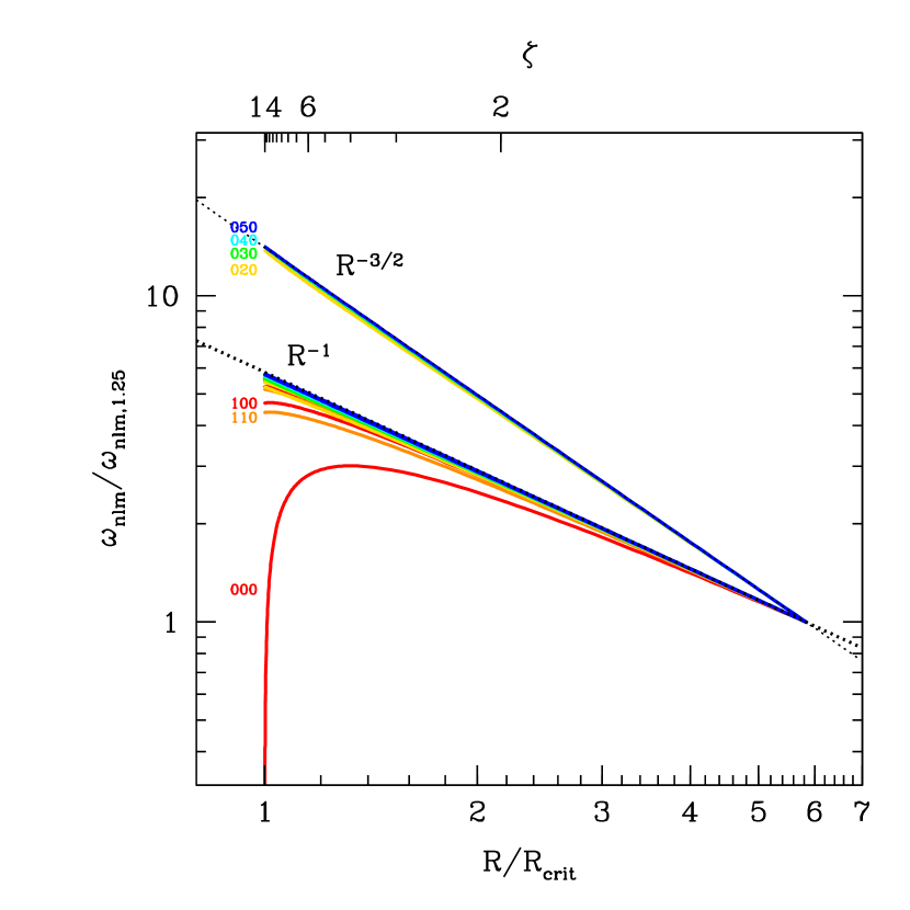
Figure 2: Normalized pulsation frequencies for a number of low-harmonic oscillations of the isothermal gas sphere as a function of sphere radius, $R$. The thick and thin black dotted line shows the $R^{-1}$ and $R^{-3/2}$, respectively. While $n=0$–$5$ and $l=0$–$5$ are shown (the frequencies are degenerate in $m$), only those that may be easily distinguished from the $R^{-1}$ asymptotic behavior are labeled. Frequencies with $l=0$, $1$, $2$, $3$, $4$ and $5$ are colored red, orange, yellow, green, cyan and blue, respectively.

Generally, $\omega_{nlm}(R)$ will depend upon the structure of the equilibrium core, in particular upon the relative sizes of the core and the wave length of the oscillations. For the oscillation modes of isothermal cores, we may construct the mode structures and compute the mode frequencies directly, shown in Figure 2 for a variety of radii (or, equivalently, $\zeta$; see, e.g., Rathore et al. 2003; Keto et al. 2006). High-order modes, i.e., modes with wavelengths much shorter than the core radius, don’t probe the gas density gradients, and we recover $\omega_{nlm}(R)\propto R^{-1}$. In contrast, low-order modes do show substantial departures from the $R^{-1}$ dependence, becoming most significant for the fundamental mode ($n=0$). For high meridional wave number ($l>1$) the fundamental modes have $\omega_{0lm}\propto R^{-3/2}$, i.e., the pulsation frequencies are roughly proportional to the Keplerian frequency at the core surface, $\omega_{K}\equiv(GM/R)^{3/2}$, corresponding to an adiabatic index of $3/2$. This is not surprising as these modes probe the radial structure of the isothermal core.

The only oscillation mode substantially deviating from either the $R^{-1}$ or $R^{-3/2}$ behaviors is the breathing mode ($n=0$, $l=0$ and $m=0$), responsible for the onset of instability at $\zeta=\zeta_{\rm crit}$, at which which $\omega_{000}$ vanishes. Near $\zeta_{\rm crit}$, $d\omega_{000}/dR$ is positive and diverges, yielding a formally infinite negative surface pressure.

2.3 The Oscillation Energy Spectrum

Once an energy spectrum, $E_{nlm}$, has been specified, we may produce a revised $P(V)$ which includes the contributions from the oscillations. This is now an explicit function of the mode amplitudes as well as $\zeta_{\rm crit}$, and thus no longer has a unique shape. In setting the $E_{nlm}$ we will have intrinsically made some statement about the mode excitation and evolution. Indeed, as we shall see in Section 4, the evolution tends to move power from small wavelengths to large wavelengths. Despite this, we may bound the likely possibilities, and already a number of important qualitative statements can be made about the dynamical importance of pulsations.

2.3.1 Large-Amplitude Monopole Oscillations

The breathing mode is unique in that, in principle, it can produce a negative contribution to the surface pressure, diverging at $\zeta=\zeta_{\rm crit}$. The breathing mode corresponds to a simple expansion and contraction of the core, similar to changing $\zeta$ in the family of equilibrium configurations. On the inward pulse, the contraction may result in $\zeta>\zeta_{crit}$ and collapse of the core. This can potentially destabilize otherwise stable isothermal cores, inducing collapse at a lower external pressure (or equivalently, smaller core mass). However, the mathematical analysis of the consequences of energetic breathing modes specifically, and monopole pulsations more generally, are not clear for a number of reasons.

Foremost among these is the failure of the linear description of the monopole oscillations. That this must happen near $\zeta=\zeta_{\rm crit}$ for the breathing mode is suggested by the fact that $\omega_{000}$ vanishes at this point, and thus $A_{000}=\omega_{000}^{-1}\sqrt{2E_{000}/M_{000}}$ diverges for finite mode energies ($M_{000}$ is not pathological at $\zeta_{\rm crit}$). More importantly, the density perturbations associated with the breathing mode diverge, doing so most strongly at the core center. Restricting our attention to pulsation amplitudes, and thus energies, for which the central density perturbation is less than the unperturbed central density (a somewhat permissive definition of “perturbation”) results in fractional changes in the supportable external pressure of less than 0.5% at all $\zeta$, and half that at most $\zeta$. That is, when we consider mode amplitudes that are indeed perturbative, the dynamical effect of the breathing mode is negligible. A similar constraint limits the dynamical importance of the higher-order monopole pulsations. Unlike the breathing mode, these generally increase the allowed external pressure, as initially anticipated. Nevertheless, as with the breathing mode, limiting their amplitudes to the perturbative regime results in a small correction to the stability of isothermal cores.

What happens in the non-linear regime is not a priori clear, and beyond the scope of this paper. However, we might expect that cores with oscillations dominated by non-linear monopole pulsations are short-lived. If non-linear monopole oscillations can indeed be excited in a subset of starless cores, and these do induce instability in a fashion similar to that anticipated by the linear analysis of the breathing mode given above, then these cores will either collapse or disperse on a single dynamical time. These cannot be the apparently long-lived cores that are observed. That is, the observed cores are necessarily those without large-scale breathing modes.

Alternatively, large-amplitude breathing modes may simply be uncommon in starless cores. If the pulsations are driven by the turbulence from the parent molecular cloud, it may be difficult to excite monopole oscillations. The intra-core motions are typically subsonic, and at the core scale, the turbulence is therefore nearly incompressible. However, the monopole modes generally, and the breathing mode specifically, are primarily compressive oscillations. Thus, the molecular cloud turbulence can only weakly couple to these oscillations, either through a small failure of the incompressible condition or through non-linear mode coupling.

For these reasons we will not consider monopole pulsations further, restricting our attention henceforth to oscillations with $l\geq 1$.

2.3.2 Non-radial Oscillations

Higher-order pulsations are nearly always stabilizing, i.e., they increase the allowed surface pressure at which stable isothermal cores exist, or alternatively increase the mass that a core can support. The exception being the $n=1$, $l=1$ oscillation which produces a small negative pressure near $\zeta_{\rm crit}$. From Equation (4) and the asymptotic behaviors of the $\omega_{nlm}$ for the non-radial oscillations, it is straightforward to estimate the contribution to the surface pressure from the oscillations:

$$P_{\rm osc}\sim\frac{E_{\rm osc}}{V}=\left|\frac{E_{\rm osc}}{E_{\rm b}}\right|\frac{E_{\rm b}}{V}\sim\left|\frac{E_{\rm osc}}{E_{\rm b}}\right|P_{0}\,,$$ (5)

where $P_{0}$ is the surface pressure of the unperturbed configuration. The precise constant of proportionality depends upon $\zeta$ and weakly on the energy spectrum.

Because for $l>0$ the form of $\omega_{nlm}(R)$ is well approximated by either $R^{-1}$ ($n>1$) or $R^{-3/2}$ ($n=0$), in practice it is not necessary to fully specify the $E_{nlm}$. Rather, it is sufficient to define $E_{\rm osc}^{0}=\sum_{n=0,l>0,m}E_{nlm}$ and $E_{\rm osc}^{>0}\equiv\sum_{n\geq 1,l>0,m}E_{nlm}$, corresponding to the energy in fundamental oscillations and the p-modes, respectively. The resulting excess pressure due to the pulsations is then

$$P_{\rm osc}\sim\frac{E_{\rm osc}^{0}}{2V}+\frac{E_{\rm osc}^{>0}}{3V}\,,$$ (6)

where $V=4\pi R^{3}/3$ and the difference between the denominators arises from the different asymptotic behaviors of the $\omega_{nlm}(R)$. Note that this is confined to the somewhat narrow range from $E_{\rm osc}/3V\leq P_{\rm osc}\leq E_{\rm osc}/2V$. While we will indeed specify the full energy spectrum, the distinction between different energy spectra will primarily be in the relative importance of $E_{\rm osc}^{0}$ and $E_{\rm osc}^{>0}$.

The particular form of the energy spectrum reflects both the mechanism by which the pulsations are excited and their subsequent evolution within the core. Here we consider three different forms for the turbulent energy spectrum, seeking to bracket the possible consequences. A natural place to begin is to assume a Kolmogorov spectrum for the oscillations, i.e.,

$$E_{nlm}^{K}\propto\left\{\begin{array}[]{ll}\displaystyle k_{nlm}^{-11/3}&\quad{\rm if~{}}l>0\\ 0&\quad{\rm otherwise}\end{array}\right.$$ (7)

where

$$k_{nlm}=\frac{\pi}{R}\sqrt{1+n^{2}+l(l+1)}\,,$$ (8)

so that $E_{k}=4\pi k_{nlm}^{2}E_{nlm}^{K}\propto k^{-5/3}$. Despite the heavy weight upon long-wavelengths, this is dominated by $n>0$ modes, primarily due to the dipole and quadrupole oscillations, such that we have $E_{\rm osc}^{>0}/E_{\rm osc}^{0}\simeq 3.5$. For concreteness, in Figure 1 the resulting surface pressure is shown by the red line for $E_{\rm osc}=0.3E_{\rm b}$, though this scales linearly with $E_{\rm osc}/E_{\rm b}$.

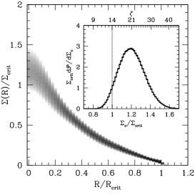
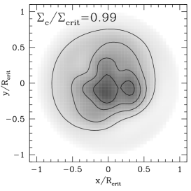
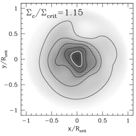
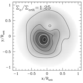
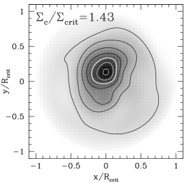
Figure 3: Column density profiles and representative maps for pulsating cores with $\zeta=14$, $E_{\rm osc}=0.3E_{\rm b}$ and a Kolmogorov energy spectrum (Equation 7). Upper Left: Probability distribution of the azimuthally-averaged column density distribution, normalized by the central column density of the critical isothermal core of the same mass. The gray-scale is logarithmic, with the floor at a probability density of 0.01. The inset shows the probability distribution of the central column density. For reference the central column density of the static configuration is also shown. On the top axis the $\zeta$ corresponding to a static isothermal core with the same mass is shown. Bottom Left: Isothermal core profiles (dashed red lines, from bottom to top, $\zeta=6$, $10$, $18$, $22$, $26$ & $30$; and solid red line, $\zeta=14.04$) and illustrative core profiles (green dotted lines) for cores with the central column densities at which the cumulative probability equals 5%, 35%, 65% & 95%, shown explicitly in the inset. Center & Right: Example column density maps, corresponding to the profiles shown in the lower left panel. The gray-scale ranges from $\Sigma/\Sigma_{\rm crit}=0$ to $1.5$, and subsequent contours are separated in steps of 0.2, with black contours for values less than unity and white above.

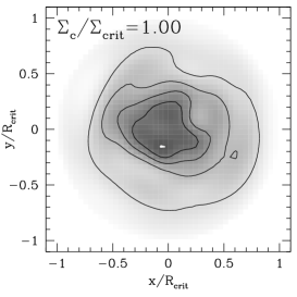
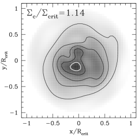
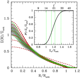
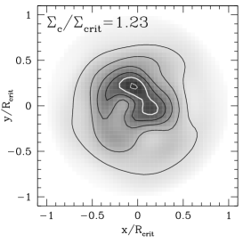
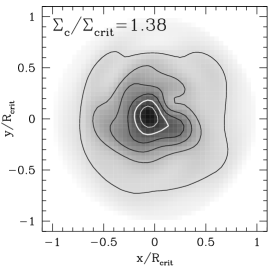
Figure 4: Column density profiles and representative maps for pulsating cores with $\zeta=14$, $E_{\rm osc}=0.3E_{\rm b}$ and a Flat energy spectrum (Equation 9). For further details see Figure 3.

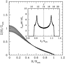
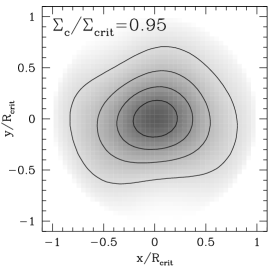
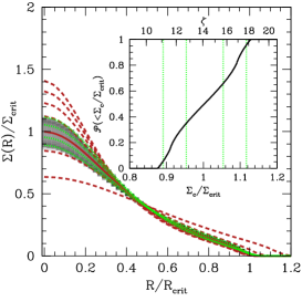
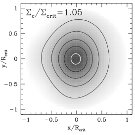
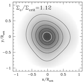
Figure 5: Column density profiles and representative maps for pulsating cores with $\zeta=14$, $E_{\rm osc}=0.3E_{\rm b}$ and a fundamental-Kolmogorov energy spectrum (Equation 10). Note the change in scale in the left-panel insets. For further details see Figure 3.

While not motivated by any particular turbulence model, a flat energy spectrum does have the virtue that all realistic choices for the turbulent spectra lie between it and the Kolmogorov distributions. Therefore, we also consider,

$$E_{nlm}^{F}\propto\left\{\begin{array}[]{ll}\displaystyle k_{nlm}^{-2}&\quad{\rm if~{}}n\leq 5~{}{\rm and}~{}0<l\leq 5\\ 0&\quad{\rm otherwise,}\end{array}\right.$$ (9)

which is flat for $n,l\leq 5$ and vanishing otherwise. The truncation is arbitrary, here set by numerical convenience. However, as argued above, the particulars of the cut-off are not important in practice since it is primarily the relative values of $E_{\rm osc}^{0}$ and $E_{\rm osc}^{>0}$ that matter. As with the Kolmogorov spectrum the latter dominates with $E_{\rm osc}^{>0}/E_{\rm osc}^{0}\simeq 3.9$ implying that the resulting perturbation to the surface pressure will be similar. Indeed, despite the considerable difference in their particulars, since $E_{\rm osc}^{>0}/E_{\rm osc}^{0}$ are similar for both spectra the resulting surface pressures are nearly indistinguishable. The surface pressure for the Flat energy spectrum is shown in Figure 1 by the blue line (when $E_{\rm osc}=0.3E_{\rm b}$). For both cases we find $P_{\rm osc}/P_{0}\simeq 0.5\left|E_{\rm osc}/E_{\rm b}\right|$, implying that the fractional change in the maximum stable mass of an oscillating isothermal core is approximately $0.25\left|E_{\rm osc}/E_{\rm b}\right|$.

Finally, we consider a fundamental-dominated energy spectrum, i.e., one in which only the $n=0$ modes are excited, with an otherwise Kolmogorov spectrum, as described for $E_{nlm}^{K}$. That is,

$$E_{nlm}^{fK}\propto\left\{\begin{array}[]{ll}\displaystyle k_{nlm}^{-11/3}&\quad{\rm if~{}}n=0~{}{\rm and}~{}l>0\\ 0&\quad{\rm otherwise}\end{array}\right.$$ (10)

Aside from presenting an extreme alternative, such an energy spectrum will be motivated in Section 4, where we discuss the evolution of the energy spectrum during core formation. In this case $E_{\rm osc}=E_{\rm osc}^{0}$ explicitly, and the resulting surface pressure, shown by the green line in Figure 1 (again for $E_{\rm osc}=0.3E_{\rm b}$), is substantially larger than those produced by the previous two spectra. This is a result of both the dependence of $P_{\rm osc}$ upon the division of energy between $E_{\rm osc}^{0}$ and $E_{\rm osc}^{>0}$ as well as the departure from the asymptotic expressions of the $\omega_{nlm}$ near $\zeta_{\rm crit}$ for $n>0$. As a consequence, in this case we find $P_{\rm osc}/P_{0}\simeq 1.0\left|E_{\rm osc}/E_{\rm b}\right|$, corresponding to a fractional increase in the maximum stable mass of approximately $0.5\left|E_{\rm osc}/E_{\rm b}\right|$.

In summary, we have found that the non-radial oscillations generally produce an increase in the surface pressure of the isothermal cores, with magnitude linearly related to the total energy in the pulsations and bounded near $\zeta_{\rm crit}$ by

$$0.5\left|\frac{E_{\rm osc}}{E_{\rm b}}\right|\lesssim\frac{P_{\rm osc}}{P_{\rm crit}}\lesssim 1.0\left|\frac{E_{\rm osc}}{E_{\rm b}}\right|\,,$$ (11)

for an extraordinarily broad class of energy spectra. This corresponds to an increase in the maximum mass of stable cores of approximately

$$0.25\left|\frac{E_{\rm osc}}{E_{\rm b}}\right|\lesssim\frac{\Delta M}{M_{\rm crit}}\lesssim 0.5\left|\frac{E_{\rm osc}}{E_{\rm b}}\right|\,.$$ (12)

3 The Structure of Mode-Supported
Equilibrium Configurations

Thus far we have characterized the effects of oscillations in terms of the unperturbed core parameters. However, large-amplitude pulsations can dramatically alter the observed appearance of a core, with important consequences for the interpretation of starless core statistics. In Keto & Field (2005), Keto et al. (2006), and Broderick et al. (2007) we showed how pulsations alter the molecular line profiles and widths. Here we explore how pulsations modify the apparent core column density profiles, $\Sigma(R)$. In this section we study the range of perturbed $\Sigma(R)$, finding that generally these are substantially asymmetric, frequently devolving into many peaked structures, and are biased towards azimuthally-averaged profiles that are best fit with super-critical static isothermal configurations. That is, stable, pulsating starless cores will typically appear to be strongly asymmetric and super-critical if fit with a static BE model.

3.1 Generating Column Densities of Pulsating Cores

To ascertain the typical observational consequences of the oscillating cores, we generate an ensemble of pulsating cores. We do this for each of the energy spectra described in Section 2.3 by setting the density to

$$\rho(\mbox{\boldmath$\rm r$})=\rho_{0}(\mbox{\boldmath$\rm r$})+\Re\left[\sum_{nlm}\sqrt{\frac{2E_{nlm}}{M_{nlm}\omega_{nlm}^{2}}}{\rm e}^{i\Phi_{nlm}}\rho_{nl}(r)Y_{lm}(\mbox{\boldmath$\rm\hat{r}$})\right]\,,$$ (13)

where the $\rho_{0}(\mbox{\boldmath$\rm r$})$ is the unperturbed density, $\rho_{nl}(r)Y_{lm}(\mbox{\boldmath$\rm\hat{r}$})$ are the density perturbation eigenfunctions and the $\Phi_{nlm}$ are randomly determined phases, corresponding to a random realization of the particular oscillations. Any realization for which $\rho(\mbox{\boldmath$\rm r$})$ vanishes anywhere is discarded, though this has little effect upon the statistical quantities since the distribution of the various observables is nearly identical for the accepted and discarded cores.

We do not vary the $E_{nlm}$, nor do we consider different underlying equilibrium configurations, choosing for concreteness a stable configuration, near critical, with $\zeta=14$. Since we vary only the phases, $\Phi_{nlm}$, we are not producing a complete ensemble; such an ensemble would necessarily have variations in the amplitudes of the oscillations, the total oscillation energy and the core masses, in addition to the mode phases. Rather, in the absence of strong constraints upon those quantities, we restrict ourselves to highlighting the consequences of the pulsations upon the measured densities with fixed amplitudes and core masses.

Once we have generated a $\rho(\mbox{\boldmath$\rm r$})$ we construct the column density map, $\Sigma(\mbox{\boldmath$\rm R$})$, by integrating along the z-axis. These are normalized to the central column density of the static, critical configuration, $\Sigma_{\rm crit}$. While the center of the unperturbed core is always located at the origin, we define the “central” column density, $\Sigma_{c}$, to be $\max\left[\Sigma(\mbox{\boldmath$\rm R$})\right]$, corresponding to how the center of the core would be defined in practice. Thus, configurations which have $\Sigma_{c}/\Sigma_{\rm crit}>1$ appear to be super-critical.

Finally, we produce azimuthally-averaged column density profiles, $\Sigma(R)$, by averaging in concentric annuli about the peak column density. Since the perturbations can both raise and lower $\Sigma(\mbox{\boldmath$\rm R$})$, this observationally motivated definition of $\Sigma_{c}$ necessarily biases us towards higher column densities, and thus towards identifying pulsating cores as closer to super-critical than the are.

We repeat this process many times, building up a statistical description of the pulsating core column densities. The results are summarized for $E_{\rm osc}=0.3E_{\rm b}$ in Figures 3–5, and are discussed in detail below.

3.2 Central Column Densities

The probability of measuring a given central column density is shown in the inset of the upper-left panel of Figures 3–5. In all cases this probability is broadly distributed about $\Sigma_{c}/\Sigma_{\rm crit}=1$. As with their dynamical consequences, the distributions arising from pulsations with Kolmogorov ($E_{nlm}^{K}$) and Flat ($E_{nlm}^{F}$) energy spectra are quite similar. Both probability distributions are centrally peaked at a value significantly larger than unity, $\Sigma_{c}/\Sigma_{\rm crit}\simeq 1.2$, corresponding to a $\zeta\simeq 21$, with only a roughly 5% probability of finding $\zeta\leq\zeta_{\rm crit}$ (seen in the cumulative probability distribution in the inset of the lower-right panels of Figures 3–5). Furthermore, these can appear to be extraordinarily super-critical, exhibiting $\zeta$’s of up to 28 for $E_{\rm osc}=0.3E_{\rm b}$.

Differing from these qualitatively, the distribution arising from the fundamental-Kolmogorov energy spectrum ($E_{nlm}^{fK}$) is double peaked. This is due to the dominance of the fundamental quadrupole mode (the dipole has no fundamental). It is also nearly symmetrically distributed about $\Sigma_{c}/\Sigma_{\rm crit}=1$, somewhat more narrowly than with the Kolmogorov and Flat spectra, and with ${\mathscr{P}}(\zeta\leq\zeta_{\rm crit})\simeq 50\%$. Despite this, the double peaked nature of the distribution implies that most cores will appear to have $\zeta$’s significantly larger or smaller than $\zeta_{\rm crit}$, reaching up to roughly $17$ for $E_{\rm osc}=0.3E_{\rm b}$.

3.3 Column Density Profiles

The results from the central column densities are borne out by the azimuthally averaged column density profiles. As before, the Kolmogorov and Flat energy spectra produce quantitatively similar results. The probability distributions of $\Sigma(R)/\Sigma_{\rm crit}$ are shown in the leftmost two panels in Figures 3–5. Over-plotted in red within the bottom left panels are a number of static isothermal core profiles, for a number of $\zeta$. $\Sigma(R)$ for the critical case is shown by the solid line, with profiles moving upward and downward in $\zeta$ increments of $4$. In particular, the $\zeta=18$ and $22$ profiles do a fair job of fitting the averaged column density profiles, while those with significantly smaller $\zeta$ do not. For reference, profiles associated with randomly chosen examples with central densities at the 5%, 35%, 65% and 95% cumulative probabilities are shown by the green dotted lines (in each Figure, these are associated with the maps shown on the right).

The fundamental-Kolmogorov energy spectrum produces similar column density profiles. As anticipated by the $\Sigma_{c}/\Sigma_{\rm crit}$ distribution, these are centered upon the critical profile, with both low and high-$\zeta$ profiles represented. In this case the averaged profiles appear to fit the static-core profiles more accurately, though this may be due to the decreased deviation from the critical core profile.

This suggests that if observations of pulsating cores are compared to a static BE model, the observed cores will quite commonly appear strongly super-critical with $\zeta>\zeta_{crit}$ even though the cores are in no imminent danger of collapse.

3.4 Column Density Maps

Despite the approximate equivalence between the average column density profiles of stable pulsating cores and static super-critical cores, the full two-dimensional maps of pulsating cores can be dramatically asymmetric. Example column density maps, randomly chosen, are shown in the center and right columns of Figures 3–5, corresponding to the same configurations for which the azimuthally averaged distributions are shown in the bottom left panel of each Figure. These are representative of the configurations appearing at the 5%, 35%, 65% and 95% cumulative probabilities, giving some idea of how typical and, perhaps, rare cores appear.

Again the column density maps associated with the Kolmogorov and Flat energy spectra are similar, though maps associated with the former are typically more centrally concentrated. In roughly 20% and 10% of cases, for the Kolmogorov and Flat spectra, respectively, the column density maps are double-peaked.

With fewer degrees of freedom, and smaller net density variations for the same $E_{\rm osc}$, it is not surprising that the fundamental-Kolmogorov spectrum shows less small-scale structure. In most cases the column density maps are only weakly non-circular. Driving $E_{\rm osc}$ up to $0.6E_{\rm b}$ produces roughly comparable variations in $\Sigma_{c}/\Sigma_{\rm crit}$, and correspondingly larger deviations from cylindrical symmetry, typically with aspect ratios larger than 2.

Nevertheless, for all three energy spectra considered it is possible to produce manifestly asymmetric structures, comparable to those observed. As a consequence, strong departures from symmetry in the column densities are not generally evidence for unstable structures.

4 Evolution of Mode-Supported Starless Cores

In addition to the excitation mechanism, the evolution of the underlying core properties and the non-linear damping of oscillations can imprint themselves upon the pulsation energy spectrum. Ultimately, the relative importance depends upon the relationship between the timescale associated with each process. Here we present some observationally motivated constraints and discuss the consequences for the stability and appearance of starless cores. In particular we motivate a picture in which the oscillations are inherited from the parent molecular cloud turbulence, and the fundamental modes are amplified at the expense of shorter wave length during a slow contraction phase resulting in a fundamental-mode dominated spectrum. Subsequent non-linear decay of the pulsations then eliminates the additional turbulent support leading to collapse and star formation in those cores that are super-critical with respect to the static BE model.

4.1 Timescales

The relevant timescales for the oscillating starless cores are the evolution timescale of the core, $T$, the pulsation periods, $P_{nlm}$, lifetimes, $\tau_{nlm}$, and excitation timescale $t_{e}$. Even without knowing the excitation mechanism we can begin to place these into a hierarchy based upon the observation that cores with large-amplitude, long-period pulsations exist. In addition to the observations of Lada et al. (2003), Redman et al. (2006) and Aguti et al. (2007) mentioned in the introduction, the observations of Sohn et al. (2007) find that about 2/3 of all their 85 observed cores show clear evidence of either expansion or contraction. Most of the remaining 1/3 show complex spectral line profiles that also indicate internal motions but are difficult to characterize. The presence of coherent oscillations immediately implies that $P_{nlm}<T,\,\tau_{nlm},\,t_{e}$. That is, for coherent oscillations to exist the core must persist in a fixed state sufficiently long for the pulsation to coordinate the large-scale motions throughout the core, and the pulsation amplitudes cannot change significantly during this process. Violations of either of these would result in motions that appear stochastic (microturbulent) instead of coherent.

That the observed pulsations have $E_{\rm osc}\sim E_{\rm b}$ implies $\tau_{nlm}\lesssim t_{e}$. Were the observed modes the result of a prolonged excitation, or many individual excitation events, we would expect with near unit probability that a given core will have had a sequence of excitations resulting in $E_{\rm osc}\gg E_{\rm b}$, at which point the core is torn apart, in direct conflict with the observation of numerous cores with substantial internal motions. In principle, this can be prevented by limiting the energy transfer during each excitation event. However, in that case the development of large-scale pulsations is itself rare, again in direct conflict with observations. Thus, as long as the excitation mechanism is uncorrelated with the pulsations themselves, i.e., there is no oscillation “feedback”, a given mode must have, on average, originated from only a single excitation event.

Finally, we have $T\lesssim\tau_{nlm}$. As the pulsations damp away, the support arising from the oscillations is lost, forcing the core to evolve towards higher central densities and then ultimately towards collapse. Thus, for cores in which the pulsations are dynamically important the mode lifetimes set an upper limit upon the core evolution time; a core may evolve on shorter timescales but it will evolve as modes decay.

Thus, in summary, the very presence of starless cores with dynamically significant pulsations gives the following hierarchy among the relevant timescales:

$$P_{nlm}<T\lesssim\tau_{nlm}\lesssim t_{e}\,.$$ (14)

This simplifies dramatically the determination of the consequences of mode decay and core evolution.

4.2 Energy Spectrum from Inherited Turbulence

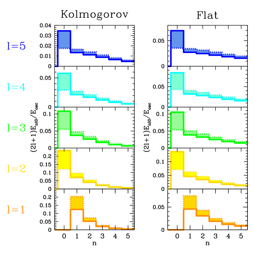
Figure 6: Evolution of the pulsation energy spectra during adiabatic core collapse. The dotted lines show $k_{nlm}^{2}E_{nlm}/E_{\rm osc}$ for the Kolmogorov (left) and Flat (right) energy spectra, assumed to be inherited at $\zeta=1.25$, as functions of $n$ for various $l$. The solid lines show the adiabatically evolved spectra at $\zeta=14$, with in all cases the fundamental ($n=0$) modes gaining substantially more energy than the other oscillations. In the case shown, by $\zeta=8$ the spectra have nearly attained their final state, implying that even for substantially sub-critical cores, the pulsation energy spectrum can be dominated by the fundamental modes.

Given that $T\lesssim t_{e}$, we are justified in imagining that pulsations on super-critical cores are relics of the core formation process. The natural mechanism for the excitation of the oscillations is then the turbulence within the parent cloud, inherited at the formation of the core. This does not mean that the energy spectrum of an observed core is always the same as the parent cloud. If cores are formed by a prolonged collapse, the evolution of the underlying equilibrium configuration modifies the energy spectrum of the oscillations. Since $P_{nlm}<T$, this process is slow in the sense described in Section 2.2, and again we may use the adiabatic invariant $E_{nlm}/\omega_{nlm}$ to estimate the evolution of the turbulent spectrum. If this formation occurs at constant temperature and mass, the mode periods are functions of $\zeta$ alone, with the dependencies implied by Figure 2. Thus, the evolved energy spectrum is given by

$$E_{nlm}(\zeta;\zeta_{0})=E_{nlm}^{K/F}\frac{\omega_{nlm}(\zeta)}{\omega_{nlm}(\zeta_{0})}\,,$$ (15)

where $\zeta_{0}$ is the center–surface density contrast at the time that the molecular cloud turbulence was inherited. The spectrum of supersonic turbulence in larger scale molecular clouds is not well understood. Observations indicate that it is close to Kolmogorov, in the range of $\sigma\sim L^{-1/3}$ to $\sigma\sim L^{-1/2}$ where $\sigma$ is the observed velocity dispersion and $L$ the length scale. For consistency with our previous analysis, we will consider both our Kolmogorov and Flat energy spectra as the inherited spectra.

For the same reason that the fundamental modes ($n=0$) and p-modes ($n>0$) produce different contributions to $P_{\rm osc}$, an adiabatic contraction results in a fundamental-heavy energy spectrum if $\zeta_{0}$ is sufficiently small. This is shown at $\zeta=14$ in Figure 6 for both the Kolmogorov and Flat energy spectra with $\zeta_{0}=1.25$. During the collapse phase, $E_{\rm osc}^{>0}/E_{\rm osc}^{0}$ has decreased from $3.5$ and $3.9$ to $1.3$ and $1.5$ for the Kolmogorov and Flat energy spectra, respectively. Thus, while in neither case the fundamental modes dominate, in both the energy in the fundamentals and p-modes are comparable. This suggests that neither $E_{nlm}^{K}$ nor $E_{nlm}^{fK}$ may be applicable, but rather some combination of the two is appropriate for the observed pulsating starless cores. This also provides a natural explanation for the dominance of low-order modes, and in particular low-order quadrupole modes, as implicated by self-absorbed asymmetric molecular line spectra in Barnard 68 (Lada et al. 2003; Keto et al. 2006; Redman et al. 2006; Broderick et al. 2007).

4.3 Pulsation Damping and the Onset of Instability

In Section 2 we showed how pulsations can support super-critical isothermal configurations. However, in the absence of continual excitation, these oscillations eventually decay. The manner and timescale in which large-amplitude pulsations damp depends upon the underlying core parameters and environment as well as the detailed structure of each individual oscillation and their amplitudes. In general the lifetimes are different for each mode. In our previous papers we have estimated life times for a few particular cases. Figures 2 and 5 of Broderick et al. (2007) estimate a decay time of 2 Myr for the 122 and 111 modes by mode-mode coupling. In Broderick et al. (2008), we estimate decay times of 1 Myr and 0.4 Myr by transmission to the larger scale ISM for isolated and embedded cores respectively. These examples are too few to define the decay times precisely; therefore, for simplicity, we assume that all pulsations decay exponentially with the same lifetime, $\tau\simeq 10^{6}\,{\rm yr}$, chosen to be consistent with our previous numerical simulations of the non-linear mode-mode and core-environment couplings (Broderick et al. 2007, 2008).

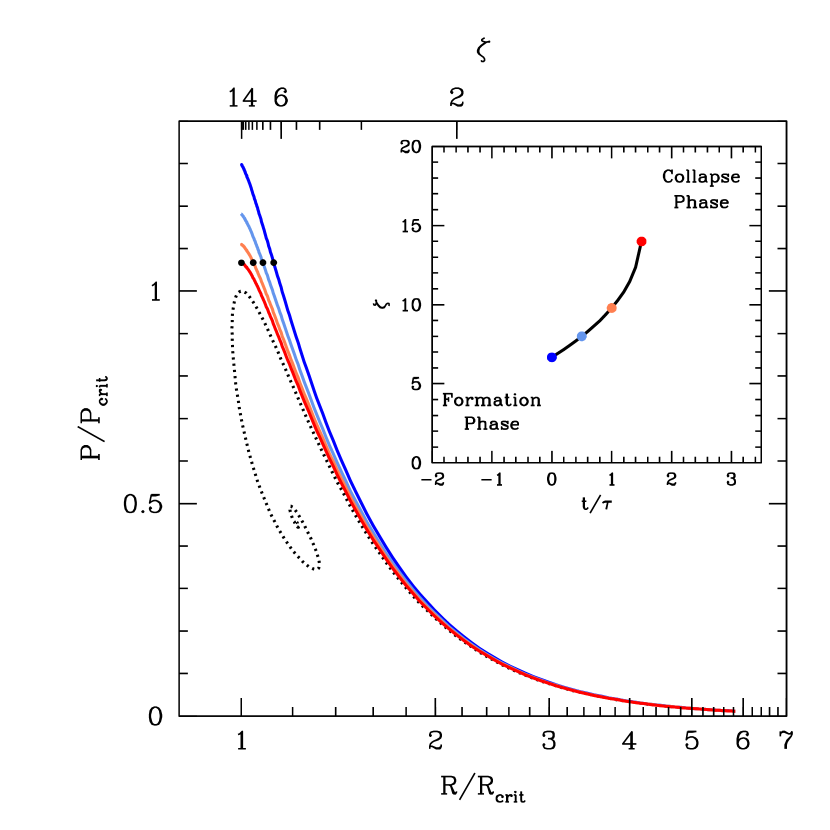
Figure 7: Surface pressure as a function of radius for an pulsating isothermal gas sphere as the oscillations decay. Initially, at $\zeta=1.25$, the gas has a Kolmogorov energy spectrum, evolving as described in Section 4.2 thereafter, and normalized such that at $t=0$ $E_{\rm osc}=0.5E_{\rm b}$ at $\zeta=14$. The pulsations energy decays exponentially in time, with decay constant $\tau$. The dark-blue, light-blue, light-red and red lines show the resulting surface pressure at $t=0$, $0.5\tau$, $1.0\tau$ and $1.5\tau$, respectively. The black points show the equilibrium configuration at a fixed, super-critical surface pressure. The inset shows time evolution of the central density. For reference, the points corresponding to the curves shown in the main figure are also plotted. Finally, the relative location of the Formation and Collapse phases are shown.

The consequences of mode damping are shown explicitly in Figure 7. Here $P(R)$ curves are shown for a number of mode amplitudes, where the energy spectrum is that resulting from a slow initial contraction period, described in Section 4.2. Initially, these are normalized such that 50% of the binding energy is in oscillations at $\zeta=14$ (dark-blue line), and then at $t/\tau=0.5$, $1.0$, and $1.5$. Since the exterior pressure is constant, we show a number of points with a fixed, super-critical surface pressure, illustrating the onset of instability during Pulsation-decay driven evolution. The associated evolution in $\zeta$, which in this case is simply proportional to the central density, is shown in the inset, with the colored points corresponding to the curves in the main Figure.

Prior to the times shown, we assume the cores were forming with $T<\tau$, presumably during a phase of prolonged contraction . At some point, due to both the increase in the dynamical importance of the pulsations and the decrease in $\tau$ due to the increased mode amplitudes and central density, the oscillations begin to dominate the formation processes, and the cores enter into a pulsation-driven phase. During this time cores can derive a substantial portion of their pressure support from the oscillations themselves, and their damping drives changes in the underlying configurations on timescales comparable to $\tau$. Finally, for super-critical cores, once the energy remaining in pulsations has reached some critical value, oscillations can no longer support the core, leading to unstable collapse. Thus, we may think of the evolution of a pulsating starless core as consisting of at least three phases: Formation, Pulsation-supported and Collapse.

4.4 Implications for the Core Mass Function

We have already used the existence of large-amplitude oscillations to empirically determine the relationship between the mode excitation timescale and the other relevant timescales. However, these timescales are not generally independent of the core mass, and may be violated for cores more massive than those observed, with consequences for the core mass function. Here we consider these within the turbulent excitation picture.

The starless cores, or their progenitors, are constantly being buffeted by the turbulence within the parent molecular cloud. The ability of a core to survive long enough to potentially form a star requires that the turbulence not excite pulsations with sufficient amplitudes to tear the core apart, either by a single catastrophic excitation or a sequence of smaller excitations. We begin by noting that in the absence of oscillations there is a well defined $M(R)$, shown in Figure 1, and at low masses roughly $\propto R^{-3/2}$. When dynamically significant oscillations are present, the core mass is a function of radius and $E_{\rm osc}$. Nevertheless, that low mass cores are generally large and vice versa. As a consequence, the binding energy of cores, comparable to $E_{\rm b}(R)\simeq GM^{2}/3R$ (within 30% at all masses), is a strong function of core mass, and in particular considerably larger for massive, compact cores.

In contrast, the energy in turbulent motions (for Kolmogorov turbulence) on the core scale is $E_{\rm t}\propto R^{2/3}$, which decreases with size. This implies that for some radius, $R_{0}$ (or mass, $M_{0}$), which depends upon the strength of the turbulence, we have $E_{\rm b}(R_{0})=E_{\rm t}(R_{0})$. Since the turbulent motions fluctuate on timescales comparable to the circulation time of a single eddy (i.e., $2\pi$ times the sound crossing time of the core), which is itself comparable to the core dynamical timescale, we expect to see at least one such excitation event for every core. For large, low-mass cores we have $E_{\rm b}<E_{\rm t}$, and we expect the core to be torn apart when this occurs, placing a lower-limit upon the mass of long-lived cores. In contrast, for compact, massive cores we have $E_{\rm b}>E_{\rm t}$, and external turbulence is no longer able to excite large-amplitude motions within the core leading again to the inherited turbulence picture described in Section 4.2.

The fact that $E_{\rm b}/E_{\rm t}\simeq(R/R_{0})^{-14/3}$ is such a strong function of $R$ implies that the range in core radii about $R_{0}$, and thus mass about $M_{0}$, in which large-amplitude pulsations can be excited is narrow. In particular,

$$\frac{\Delta R}{R_{0}}\simeq\left|\frac{d\ln R}{d\ln(E_{\rm b}/E_{\rm t})}\right|_{R=R_{0}}\simeq 0.2\quad\Rightarrow\quad\frac{\Delta M}{M_{0}}\simeq 0.3\,.$$ (16)

Cores much less massive than $M_{0}$ are torn apart, while those much more massive than $M_{0}$ never develop the observed large-amplitude pulsations. The latter issue is moderated somewhat if an adiabatic contraction phase occurs during the formation process, i.e., if the pulsation amplitude are representative of those generated when the core was considerably larger. Nevertheless, the former places a hard constraint upon the minimum mass of starless cores.

5 Conclusions

The onset of instability in isothermal gas spheres depends upon the dynamical state of the object. While this has long been known, usually within the context of effective turbulent support, how this occurs in practice depends upon the oscillation mode energy spectrum, and therefore the mechanism by which pulsations are excited. In principle, large-amplitude breathing modes can induce instability for masses well below $\zeta>4$ the static stability limit, a fact that is reflective of the nature of the instability. However, in practice, doing so requires extraordinarily non-linear mode amplitudes, at which point the dynamical effect is unclear. In contrast, higher-order pulsations are generically supportive, increasing the maximum stable mass significantly. For oscillation energies comparable to those required to explain the self-absorbed, asymmetric molecular line profiles typically observed in starless cores, the maximum stable mass is about $10$–$30\%$ higher than the static case.

If the modes are excited during the core’s formation, presumably inherited from the turbulence of the parent molecular cloud, followed by an adiabatic contraction, it is natural to expect low-$n$ oscillations to dominate the energy spectrum. That is, even prior to mode decay via mode-mode or mode-environment coupling, energy from the collapse is preferentially shunted into the long-wavelength pulsations. Thus, it is not unreasonable to expect starless cores to pulsate predominantly in low-order multipole modes, with $l\geq 2$.

The presence of large-amplitude oscillations can dramatically alter the morphology of the column density maps of starless cores, mimicking the unstable configurations of static BE spheres. For turbulent energy spectra, dynamically significant pulsations dramatically bias the maximum column densities towards larger values, with the average exceeding that associated with the critical configuration of static BE models by factors of order unity. This is born out by the azimuthally-averaged column density profiles, which are very similar to isothermal gas profiles associated with $\zeta$ above the critical value. Despite this, the two-dimensional column density maps are strongly asymmetric, featuring in some cases multiple peaks, similar to those observed in practice.

The ultimate decay of the oscillations, facilitated by non-linear mode coupling or by coupling to the surrounding molecular gas, results in the collapse of super-critical cores. For slow decay (lifetimes exceeding the mode periods) this results in a sequence of quasi-stable isothermal gas spheres, and the evolution may be determined explicitly. This assumes that the oscillations are not continually re-excited by small scale processes within or near the starless cores themselves. However, the very existence of a significant number of pulsating cores, with mode energies being a considerable fraction of the cores’ binding energy, argues against this.

Taken together, these suggest a picture of star formation, framed entirely within a hydrodynamical paradigm. Self-gravitating cores condense out of the turbulent sea within molecular clouds, born with large-amplitude pulsations. These pulsations drastically perturb the core shape, mimicking non-equilibrium structures as well as initially supporting the cores against collapse. As the oscillations decay the core becomes unstable resulting in star formation. In this scheme the rate of star formation is set not by ambipolar diffusion of a large scale magnetic field, but by the non-linear decay of the core pulsations.

We should emphasize that while we have framed this new picture entirely in terms of hydrodynamics, small scale tangled magnetic fields in equipartition with the turbulent energy are still allowed and might be required. The model of oscillations as perturbations does not allow amplitudes large enough to produce the supersonic motions occasionally seen in a few cores. These are the exception rather than the rule and might not be pulsations at all, but rather inward motions as the core center transitions to free-fall collapse. However, if these motions are sub-Alfvénic pulsations, they may be subsumed into an equivalent magnetohydrodynamic formulation, in which we consider only small-scale magnetic fields. In this case, it would be the decay of the magnetohydrodynamic pulsations, not ambipolar diffusion, that sets the star formation rate. Nevertheless, as empirical evidence accumulates for the existence of large-amplitude oscillations in starless cores, it is clear that their dynamical effects upon the cores themselves cannot be ignored.

References

- Aguti et al. (2007) Aguti, E. D. et al. 2007, ApJ, 665, 457
- Alves et al. (2001) Alves, J. F., Lada, C. J., & Lada, E. A. 2001, Nature, 409, 159
- Andre et al. (1996) Andre, P., Ward-Thompson, D., & Motte, F. 1996, A&A, 314, 625
- Bacmann et al. (2000) Bacmann, A. et al. 2000, A&A, 361, 555
- Beichman et al. (1986) Beichman, C. A. et al. 1986, ApJ, 307, 337
- Benson & Myers (1989) Benson, P. J. & Myers, P. C. 1989, ApJS, 71, 89
- Bergin & Tafalla (2007) Bergin, E. A. & Tafalla, M. 2007, ARA&A, 45, 339
- Bergin et al. (2006) Bergin, E. A. et al. 2006, ApJ, 645, 369
- Bonnor (1956) Bonnor, W. B. 1956, MNRAS, 116, 351
- Broderick et al. (2007) Broderick, A. E., Keto, E., Lada, C. J., & Narayan, R. 2007, ApJ, 671, 1832
- Broderick et al. (2008) Broderick, A. E., Narayan, R., Keto, E., & Lada, C. J. 2008, ApJ, 682, 1095
- Crapsi et al. (2007) Crapsi, A., Caselli, P., Walmsley, M. C., & Tafalla, M. 2007, A&A, 470, 221
- di Francesco et al. (2007) di Francesco, J. et al. 2007, in Protostars and Planets V, ed. B. Reipurth, D. Jewitt, & K. K. (University of Arizona Press: Tuscon), 17–32
- Dickman & Clemens (1983) Dickman, R. L. & Clemens, D. P. 1983, ApJ, 271, 143
- Evans et al. (2001) Evans, II, N. J., Rawlings, J. M. C., Shirley, Y. L., & Mundy, L. G. 2001, ApJ, 557, 193
- Field et al. (2008) Field, G. B., Blackman, E. G., & Keto, E. R. 2008, MNRAS, 385, 181
- Gingold & Monaghan (1980) Gingold, R. A. & Monaghan, J. J. 1980, MNRAS, 191, 897
- Goldstein (1980) Goldstein, H. 1980, Classical Mechanics, 2nd ed. (Addison-Wesley: Reading, Mass.)
- Gonçalves et al. (2004) Gonçalves, J., Galli, D., & Walmsley, M. 2004, A&A, 415, 617
- Jessop & Ward-Thompson (2000) Jessop, N. E. & Ward-Thompson, D. 2000, MNRAS, 311, 63
- Kandori et al. (2005) Kandori, R. et al. 2005, AJ, 130, 2166
- Keto et al. (2006) Keto, E., Broderick, A. E., Lada, C. J., & Narayan, R. 2006, ApJ, 652, 1366
- Keto & Caselli (2008) Keto, E. & Caselli, P. 2008, ApJ, 683, 238
- Keto & Caselli (2010) Keto, E. & Caselli, P. 2010, MNRAS, 402, 1625
- Keto & Field (2005) Keto, E. & Field, G. 2005, ApJ, 635, 1151
- Kirk et al. (2005) Kirk, J. M., Ward-Thompson, D., & André, P. 2005, MNRAS, 360, 1506
- Lada et al. (2003) Lada, C. J., Bergin, E. A., Alves, J. F., & Huard, T. L. 2003, ApJ, 586, 286
- Lada et al. (2008) Lada, C. J. et al. 2008, ApJ, 672, 410
- Landau & Lifshitz (1976) Landau, L. D. & Lifshitz, E. M. 1976, Mechanics, 3rd ed., ed. Landau, L. D. & Lifshitz, E. M. (Butterworth-Heinemann Ltd: Oxford)
- Myers & Benson (1983) Myers, P. C. & Benson, P. J. 1983, ApJ, 266, 309
- Myers et al. (1983) Myers, P. C., Linke, R. A., & Benson, P. J. 1983, ApJ, 264, 517
- Pagani et al. (2003) Pagani, L. et al. 2003, A&A, 406, L59
- Pagani et al. (2004) Pagani, L. et al. 2004, A&A, 417, 605
- Pineda et al. (2010) Pineda, J. E. et al. 2010, ApJ, 712, L116
- Rathore et al. (2003) Rathore, Y., Broderick, A. E., & Blandford, R. 2003, MNRAS, 339, 25
- Redman et al. (2006) Redman, M. P., Keto, E., & Rawlings, J. M. C. 2006, MNRAS, 370, L1
- Schnee et al. (2007) Schnee, S. et al. 2007, ApJ, 671, 1839
- Shirley et al. (2002) Shirley, Y. L., Evans, II, N. J., & Rawlings, J. M. C. 2002, ApJ, 575, 337
- Sohn et al. (2007) Sohn, J. et al. 2007, ApJ, 664, 928
- Stamatellos & Whitworth (2003) Stamatellos, D. & Whitworth, A. P. 2003, A&A, 407, 941
- Tafalla et al. (2002) Tafalla, M., Myers, P. C., Caselli, P., Walmsley, C. M., & Comito, C. 2002, ApJ, 569, 815
- Teixeira et al. (2005) Teixeira, P. S., Lada, C. J., & Alves, J. F. 2005, ApJ, 629, 276
- Ward-Thompson et al. (2002) Ward-Thompson, D., André, P., & Kirk, J. M. 2002, MNRAS, 329, 257
- Ward-Thompson et al. (1999) Ward-Thompson, D., Motte, F., & Andre, P. 1999, MNRAS, 305, 143
- Ward-Thompson et al. (1994) Ward-Thompson, D., Scott, P. F., Hills, R. E., & Andre, P. 1994, MNRAS, 268, 276
- Ward-Thompson et al. (2007) Ward-Thompson, D. et al. 2007, in Protostars and Planets V, ed. B. Reipurth, D. Jewitt, & K. K. (University of Arizona Press: Tuscon), 33–46
- Zucconi et al. (2001) Zucconi, A., Walmsley, C. M., & Galli, D. 2001, A&A, 376, 650