Running coupling and mass anomalous dimension of SU(3) gauge theory with two flavors of symmetric-representation fermions
Abstract
We have measured the running coupling constant of SU(3) gauge theory coupled to flavors of symmetric representation fermions, using the Schrödinger functional scheme. Our lattice action is defined with hypercubic smeared links which, along with the larger lattice sizes, bring us closer to the continuum limit than in our previous study. We observe that the coupling runs more slowly than predicted by asymptotic freedom, but we are unable to observe fixed point behavior before encountering a first order transition to a strong coupling phase. This indicates that the infrared fixed point found with the thin-link action is a lattice artifact. The slow running of the gauge coupling permits an accurate determination of the mass anomalous dimension for this theory, which we observe to be small, , over the range of couplings we can reach. We also study the bulk and finite-temperature phase transitions in the strong coupling region.
pacs:
11.15.Ha, 11.10.Hi, 12.60.NzI Introduction
Several possibilities for new physics beyond the Standard Model involve a new strongly interacting sector of gauge fields and light fermions. In the oldest such idea, technicolor, interactions are presumed to be asymptotically free at very short distance but strong at long distance, leading to a fermion–antifermion condensate that replaces the Higgs vacuum expectation value Hill:2002ap . A more recent proposal couples the standard model to a sector of “unparticles,” in which long distance dynamics is conformal in the limit of zero fermion mass Georgi:2007ek . Determining whether either of these scenarios occurs in a candidate theory is a nonperturbative question. In the last few years many groups have begun to attack it using lattice methods reviews .
One common tool for diagnosing the infrared structure of a gauge theory is its beta function. In perturbation theory it has the expansion
| (1) |
where, for an SU() gauge theory with flavors of fermions in representation ,
| (2) | |||||
| (3) |
Here is the value of the quadratic Casimir operator in representation [where denotes the adjoint representation, so ], while is the conventional trace normalization. We are interested in asymptotically free theories, so we demand to force an infrared repulsive fixed point at . If while , the two-loop beta function will have a zero Caswell:1974gg ; Banks:1981nn at some . Whether the theory is a candidate for strongly interacting dynamics or for conformal behavior at long distance scales depends on whether the complete, nonperturbative has a zero. If it does have such an infrared attractive fixed point (IRFP), then we have an unparticle theory with a scale-invariant coupling at large distances. If it does not, so that runs to strong coupling in the infrared, we have a technicolor candidate. The technicolor category also includes the possibility of a coupling region where approaches zero without crossing it. The coupling would then evolve slowly between widely differing energy scales. “Walking technicolor” is built on this scenario Holdom:1981rm ; Yamawaki:1985zg ; Appelquist:1997fp .
In a massive theory, the running coupling is supplemented by the running fermion mass . The counterpart of the beta function is the anomalous dimension of the mass operator . It determines the running of the mass parameter according to
| (4) |
If the system is conformal at zero fermion mass , then near the correlation length scales as
| (5) |
where is the leading relevant exponent of the system (in the language of critical phenomena). In lowest order in perturbation theory,
| (6) |
In the massless theories used for technicolor, governs the running of the condensate . It is thus an important diagnostic for realistic “extended” technicolor models. Phenomenological constraints on such models require it to have a large, nonperturbative value.
Briefly Chivukula:2010tn , at issue is the dual role of the conventional Higgs condensate in giving masses both to the weak bosons and to the quarks and leptons. In technicolor theories, the mass comes from the techniquark condensate ; this demands that the technicolor scale be not much above the weak scale, TeV. The light fermions, on the other hand, get their mass from joining the techniquarks in a multiplet of an extended technicolor (ETC) gauge group, which breaks to the technicolor group at scale . The coupling of the techniquark condensate to the light fermions via emission of ETC gauge bosons gives the light fermions their masses,
| (7) |
On the other hand, the exchange of ETC gauge bosons generates flavor-changing neutral currents (FCNC) among the light fermions, with effective vertices . Suppression of FCNC demands that be pushed up beyond 1000 TeV, but then the fermion masses generated by Eq. (7) come out too light, as small as MeV.
The solution of this problem in ETC theories lies in the recognition that the two uses of the condensate involve its evaluation at two very different energy scales. The weak boson masses are connected to the condensate at , while the fermion masses are determined by its value at . The condensate runs between these two scales according to its anomalous dimension, so that the numerator in Eq. (7) is really
| (8) |
If is approximately constant, then
| (9) |
Since the ratio , a “condensate enhancement” of this order can account for most quark masses—but only if is close to 1.
The walking-technicolor scenario combines a near-zero of the beta function with a large anomalous dimension for the mass. One envisions a (perhaps) rapid evolution of the coupling away from at some extremely high energy scale, which slows to near-fixed-point behavior at some moderately large coupling at scale . The coupling then runs very slowly until is reached, even as the techniquark mass runs with a large anomalous dimension . At , the coupling is a bit stronger and creates the techniquark condensate; the techniquarks thereupon decouple and the coupling runs on to strong values, leaving technicolor confined at low energies.
Most of the ingredients in this story—near-fixed-point behavior, condensation, and subsequent confinement—involve nonperturbative physics. Lattice methods, which have been fairly successful in dealing with the properties of QCD, are a natural approach to investigate them Nelson:2006zz . Every candidate model for new physics begs the two questions:
-
1.
Is the long distance dynamics of the candidate theory conformal, or confining, or something else?
-
2.
What is the value of in the interesting energy range?
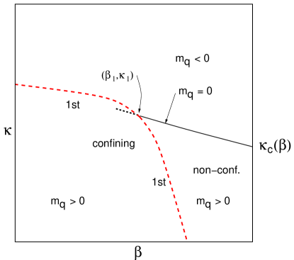
For some time our program has been to study the gauge theory proposed for “next-to-minimal” walking technicolor Sannino:2004qp ; Hong:2004td ; Dietrich:2005jn ; Belyaev:2008yj : SU(3) gauge fields coupled to two flavors of fermions in the two-index symmetric representation, which is the sextet. In Ref. Shamir:2008pb we measured the running coupling constant defined in the Schrödinger-functional background field method. We found, with the small lattices at our disposal, that the integrated beta function has a zero, indicating that the theory is in a conformal phase. In Ref. DeGrand:2008kx we performed spectroscopic studies in the theory with non-zero quark mass. We observed two phases for the system in finite volume: a strong-coupling, confined phase and a weakly coupled, chirally restored phase. (See Fig. 1. The massless curve is where our Schrödinger functional calculations are done.) While one might interpret the two phases as low- and high-temperature phases, the phase transition in the massless theory [i.e., at ] appeared not to move as the lattice volume increased; this is in marked contrast to the usual high-temperature phase transition in confining gauge theories.
Following these calculations, we changed the lattice action from the usual Wilson–clover action (“thin links”) to an improved action, incorporating normalized hypercubic smearing (“nHYP fat links”) that has shown dramatic reduction of lattice artifacts when used for QCD simulations. One of us DeGrand:2009hu performed a finite-size scaling analysis of correlation lengths in the weak coupling phase, approaching the massless curve. A small anomalous dimension, , was observed at two values of the bare parameters.111For other recent work on SU(3) gauge theory with sextet fermions, see Fodor:2009ar ; Machtey:2009wu ; Kogut:2010cz .
In this paper we report on a new calculation of the running coupling constant and of the mass anomalous dimension, using the improved action on lattice volumes larger than in Refs. Shamir:2008pb ; DeGrand:2008kx . The first step is to determine the phase structure of the lattice theory. As with the original, thin-link action, the improved, fat-link action has a confined phase in which it is not possible to tune the quark mass to zero. We go beyond Ref. DeGrand:2008kx in studying closely the region where the line intersects the phase boundary, and we find that there is no critical point. The phase boundary moves up the curve very slowly as the simulation volume grows; it is also affected by the choice of boundary conditions. As noted in the context of other, similar gauge theories (e.g., Iwasaki:2003de ), this phase diagram is different from that of QCD and it is hard to see how it can tend to a confining theory in the continuum limit. Such considerations, however, are far from conclusive.
Turning to the SF calculation, we find that the coupling constant runs more slowly than two-loop perturbation theory would predict. This is such slow running that we are unable to chain together results from different sets of bare parameters to construct a picture of running over decades of the length scale . The range of couplings that we can investigate is limited by the strong-coupling phase transition. The beta function might cross zero at the strongest coupling that we can reach, but we cannot make a strong claim to this effect.
Our previous calculation Shamir:2008pb , with the thin-link action, was unable to pursue the function to SF couplings stronger than because of the transition to the strong-coupling phase. The infrared fixed point found in that work was at a renormalized coupling (see Fig. 7 below), which was uncomfortably close to the transition. With the fat-link action we are able to push the transition to , so that the region around is well insulated from lattice artifacts. Thus the present calculation is more reliable when it rules out the fixed point found previously.
As part of the SF calculation, we compute the anomalous dimension . Even when one takes into account possible finite-lattice effects, the result has much smaller uncertainty than the calculation of Ref. DeGrand:2009hu and confirms its conclusion: is small over our observed range of couplings.
The outline of the paper is as follows: In Sec. II we review our lattice action and the techniques we use to measure the beta function and . In Sec. III we describe our studies of the boundary between the strong- and weak-coupling phases. Sections IV and V contain our results for the running coupling constant and mass anomalous dimension. We summarize the calculation in Sec. VI, and place it in context of other lattice calculations. The appendix contains data that support our determination of the phase boundary as presented in Sec. III.
II Methodology
II.1 Lattice action and simulation
We study the SU(3) gauge theory with two flavors of dynamical fermions in the sextet representation of the color gauge group. The lattice action is given by the single-plaquette gauge action and a Wilson fermion action with added clover term Sheikholeslami:1985ij . The gauge connections in the fermion action employ the differentiable hypercubic smeared link of Ref. Hasenfratz:2007rf , from which the symmetric-representation gauge connection for the fermion operator is constructed. The parameters that are inputs to the simulation are the bare gauge coupling and the fermion hopping parameter , related to the bare mass by . Unlike our earlier calculation with the thin-link fermion action, no tadpole improvement is necessary here and thus we set the clover coefficient to its tree-level value (i.e., unity). The smearing parameters for the links are the same as in Ref. Hasenfratz:2007rf : , , .
The molecular dynamics integration is accelerated with an additional heavy pseudo-fermion field as suggested by Hasenbusch Hasenbusch:2001ne , multiple time scales Urbach:2005ji , and a second-order Omelyan integrator Takaishi:2005tz . Lattice sizes range from to sites; some data for the phase diagram were obtained with lattices of sites.
II.2 Why fat links?
The simulations we reported in Ref. Shamir:2008pb were performed using the usual clover action Sheikholeslami:1985ij in which the coefficient of the clover term was adjusted via tadpole improvement. When we began the present set of simulations, we were faced with a choice: either to continue using the same action and simply to push to larger lattice volumes, or to attempt as well to improve the action further. We chose the latter course.
Improvement criteria are basically identical for any asymptotically free theory. As one tunes the bare coupling toward zero, the lattice theory should have an expansion in powers of the lattice spacing . The dimension-four terms in this expansion are identical to those of a continuum action, while the higher-dimensional terms, which are multiplied by positive powers of the lattice spacing, correspond to irrelevant operators. The inclusion of a clover term, for instance, allows the fermion action to be free of artifacts if the clover term is appropriately chosen. In general, the particular choice of lattice discretization is formally irrelevant. In practice, however, it will make a big difference in terms of eliminating lattice artifacts. We chose hypercubic smeared links because of our positive experience with them in QCD simulations.
Fermionic actions with hypercubic smeared links have a number of favorable features, which we enumerate in the context of the present simulation:
-
1.
The gauge fields seen by the fermions are smoother with a smeared link than they are with a thin link. The plaquette (in the fermions’ color representation) is a rough indicator of this. For example, at the thin-link (fundamental) plaquette has a value of about 0.43 (normalized to a maximum of 1) while the sextet-representation smeared-link plaquette is about 0.78 (normalized likewise). Thus, even at this strong (bare) coupling, one can imagine expanding the link variable in order to recover the continuum action.
-
2.
The value of , at which the quark mass (see below) vanishes, is closer to the free-field value of 1/8 with smeared links than it is in our original thin link calculation. Even at the boundary of the strong-coupling phase we find , versus a range of 0.15–0.17 for the entire range of couplings studied in the thin-link theory in Ref. Shamir:2008pb .
-
3.
Tests with quenched fundamental fermions Hoffmann:2007nm reveal that the nonperturbatively improved clover coefficient is very close to its tree level value at fairly large lattice spacings. Preliminary results show this to be the case in the present theory as well evgeny . This is our justification for setting here.
-
4.
Finite renormalization factors for (partially) conserved currents are much closer to unity than for the thin-link clover action. This is easily checked in one-loop perturbation theory, where the vector and axial-vector lattice-to-continuum renormalization factors are , where is a pure number, a lattice integral DeGrand:2002vu .
While the formal arguments for improvement via smearing may be called into question outside the weak-coupling limit, the practical observations listed above justify its application and show why results from the smeared theory are more reliable than those obtained without smearing. Nonetheless, asymptotic freedom does underlie the whole philosophy. If an infrared fixed point were to be found, the theory on the strong-coupling side of the fixed point would not be asymptotically free. Little is known a priori about such a strong-coupling theory.
As mentioned in the introduction, we find in the present study that the use of hypercubic smeared links allows us to reach a much larger value of the Schrödinger functional coupling than we could get to in Ref. Shamir:2008pb , versus about 2.5, before encountering the strong-coupling phase transition. Thus the region , where the thin-link calculation indicated an infrared fixed point, can be studied more reliably.
II.3 Schrödinger functional method and the running coupling
The Schrödinger functional (SF) Luscher:1992an ; Luscher:1993gh ; Sint:1995ch ; Jansen:1998mx method is an implementation of the background field method that is especially suited for a lattice calculation. Taking the simulation volume to be a 4-cube of dimension , one imposes fixed boundary conditions on the gauge field at and while imposing periodic boundary conditions in the spatial directions. The classical field that minimizes the Yang–Mills action subject to the fixed boundary conditions is a background color-electric field. By construction the only distance scale that characterizes the background field is , so the -loop effective action gives the running coupling via
| (10) |
where
| (11) |
is the classical action of the background field. When is calculated non-perturbatively, Eq. (10) gives a non-perturbative definition of the running coupling at scale .
Since in a lattice calculation one cannot calculate itself, one differentiates Eq. (10) with respect to some parameter in the boundary conditions. Thus
| (12) |
The derivative of gives an observable quantity, while is just a number Luscher:1993gh . We choose boundary fields as described in Ref. Jansen:1998mx ; for these boundary values the coefficient . The observable,
| (13) |
is a particular expectation value of the gauge fields and the Dirac operator . The parameter enters linearly into phase angles so the derivatives on the right-hand side of Eq. (13) are implemented by putting the appropriate fixed values in place of the boundary links Luscher:1993gh . We also impose twisted spatial boundary conditions on the fermion fields as suggested in Ref. Sint:1995ch , , with on all three axes DellaMorte:2004bc .
The observable (13) is quite noisy and requires long simulation runs, as shown in Table 1. The acceptance in the hybrid Monte Carlo simulations was kept at 80–90%, except at the strongest couplings for where we were forced to use short time steps even to reach acceptances as low as 40%.
| trajectories | |||||
|---|---|---|---|---|---|
| 5.8 | 0.12835 | 8 000 | 2 300 | 10 000 | – |
| 5.4 | 0.12920 | 8 000 | 3 050 | 9 600 | – |
| 5.0 | 0.13062 | 13 000 | 6 030 | 8 800 | – |
| 4.8 | 0.13173 | 45 000 | 5 250 | 16 700 | – |
| 4.6 | 0.13320 | 74 000 | 13 400 | 11 300 | 22 400 |
| 4.4 | 0.13510 | 67 200 | 22 900 | 11 300 | 29 200 |
| 4.3 | 0.13617 | 14 800 | 15 600 | 8 000 | 6 750 |
II.4 Anomalous dimension
The mass anomalous dimension is determined from the volume dependence of the renormalization factor of the isovector pseudoscalar density . (The latter is related by a chiral rotation to , which is the object of interest.) It is computed from two correlators via Sint:1998iq ; Capitani:1998mq ; DellaMorte:2005kg ; Bursa:2009we
| (14) |
is the propagator from the boundary to a point pseudoscalar operator at time ,
| (15) | |||||
and we take ; here and are gauge-invariant wall sources at , meaning one lattice layer away from the boundary. The normalization of the wall source is removed by the factor, which is the boundary-to-boundary correlator,
| (16) | |||||
where and are wall sources at . The constant allows imposing a volume-independent normalization condition in the weak-coupling limit.
In SF calculations for QCD, correlators such as (15) and (16) are usually computed with the spatial link matrices at and set to unity. This is because it is desired to compute with an absolute normalization (to fix the physical value of a quark mass, for example). Correspondingly, the constant that normalizes has only been calculated for these boundary conditions. Since our interest, however, is in how runs with the scale , we will calculate only ratios of values of for different at fixed lattice couplings. Because of this, the overall normalization of is irrelevant. We are thus free to ignore and also to use the same boundary conditions for the calculation of as for the simulations which generated the data for the SF coupling. Thus the data for came from the same configurations as the coupling calculation, effectively giving for free. We set in tabulating below.
II.5 Quark mass
We studied the massless theory by fixing , the point at which the quark mass vanishes for each . We define using the unimproved axial Ward identity (AWI),
| (17) |
where and could be any source. We follow the usual SF procedure and take the source to be the gauge-invariant wall source at as in Eq. (15). The correlation functions in Eq. (17) are then measured at , the midpoint of the lattice. The derivative is taken as the symmetric difference, .
III Strong coupling
III.1 First-order phase boundary
As shown in Fig. 1, both the thin-link and the fat-link lattice theories show a first-order phase transition separating a low- (strong bare coupling) phase from a high- (weak bare coupling) phase. Our work on the thin-link DeGrand:2008kx and fat-link DeGrand:2009hu theories showed that:
-
•
The low- phase is confining, as revealed by the heavy-quark potential (for sources in the fundamental representation).
-
•
The high- phase is chirally restored, as revealed by parity doubling between the scalar and pseudoscalar masses, and also between the vector and axial-vector masses. The string tension is unobservably small in this phase.
-
•
In the high- phase, all screening masses and the pseudoscalar decay constant fall towards zero as , until the correlation length () approaches , the length of the lattice in a direction transverse to the direction in which the correlator is measured. Then plateaus at a value proportional to . This behavior superficially resembles the usual finite-size scaling for a critical system in finite volume, where plays the role of a relevant perturbation Cardy:1996xt . (This behavior was exploited in Ref. DeGrand:2009hu .)
While the two phases appear for both SF boundary conditions and for the usual thermal [i.e., (anti-)periodic temporal] boundary conditions, there are important differences between the two cases. For thermal boundary conditions (BC) the Polyakov loop (in the fundamental representation) can be used as usual to distinguish between the two phases. In the strong-coupling phase it is near zero, real and slightly negative. (It will be recalled that the fermion action with thermal BC breaks the global Z(3) symmetry of the gauge action.) In the weak-coupling phase the Polyakov loop orders along one of the Z(3) center elements. The state with real and positive is the stable one, while the states which order along the other directions, , are metastable.222 We observed tunneling among these states on lattices with volume . See Ref. Machtey:2009wu for a study of the thin-link theory, and compare Kogut:2010cz . This allows the characterization of the phase transition as a finite-temperature confinement transition, as far as is possible in a theory with dynamical fermions.
With SF boundary conditions (SFBC), on the other hand, the fermion action does not break the Z(3) center symmetry—the Z(3) symmetry is exact, just as in the pure gauge theory. As it turns out, the Z(3) symmetry is spontaneously broken in the weak-coupling phase; it is unbroken in the strong-coupling phase, so that ¡P¿=0 there, much the same as in a pure gauge theory with thermal BC. Of course, a gauge theory with SFBC has no interpretation as a true finite-temperature system.
In both cases, the entire phase boundary is strongly first-order, as seen in discontinuities in the plaquette, in the AWI quark mass, in the ordering of the Polyakov loop, and, most of all, in hysteresis. Simulations initialized in one phase but run at parameters in the other phase can run for hundreds of molecular dynamics time steps without tunneling. We present plots of the mean plaquette and the AWI quark mass in the appendix.
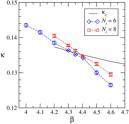
We located the phase boundary by performing simulations with mixed starts—one half of the initial gauge configuration is taken from an equilibrium configuration at some in one phase, while the other half is from an equilibrium lattice at in the other phase. We then watch the system equilibrate. This can be quite expensive, as it requires tiny time steps to avoid rejection of the molecular dynamics trajectory in the HMC algorithm. We have thus only done these tests for lattices of temporal extent and 8: , , and lattices with SFBC, and and lattices with thermal BC. The location of the phase boundary depends on the choice of BC as well as on . We show the region of the intersection of the phase boundary with the curve for the various cases in Figs. 2 and 3.
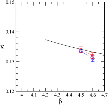
It should not be surprising that the phase boundary shifts when SFBC are replaced by thermal. For given , thermal lattices have spacelike layers of dynamical links, while SF lattices have only . The smaller number of dynamical degrees of freedom means that the SF lattice is effectively at a higher “temperature” than the thermal lattice at the same . Indeed, comparison of Figs. 2 and 3 shows that the phase boundary for the SF theory lies below and to the left of that of the thermal theory with the same . This behavior is familiar in thermal gauge theories when is varied. We repeat, however, that the SF theory is not a finite-temperature theory and that the phase transition in the SF theory is not a finite-temperature transition.
We performed SF calculations on the line, defined by . In the weak coupling phase it is quite easy to find , and its volume dependence is small. When is less than , the gauge coupling where the line meets the first order line, the quark mass is never zero; it changes sign discontinuously when crosses the phase boundary (see the appendix). This means that there is no massless theory to the left of . The curve can, however, be extended leftward into the strong-coupling phase by simulating in the metastable state, which is continuously connected to the weak-coupling phase. It is in fact possible to do long runs in this state without tunneling out if it. We can calculate , which does cross zero and thus gives us ; we can also calculate and . As we will show, these observables remain very similar to their values in the region of bare parameter space where the weak-coupling phase is the true vacuum.
There is another metastable extension of the line, found by following a confining state into the non-confining phase. We have not explored this because simulation in confining states is much more difficult.
III.2 Shift of the phase boundary with lattice size
For the phase boundary shifts to the right as is increased. For sufficiently small this is to be expected since this is the scaling behavior typical of the finite-temperature transition when the fermions are massive. It turns out to be true for as well. Close to , this shift is very small. One interpretation of the lack of motion of the phase boundary here is that, close to this point, the transition is a bulk transition, weakly affected by the finite size of the lattice. The alternative explanation is that (at least for thermal boundary conditions) the transition is still a finite temperature transition, but that it is moving very slowly.
To appreciate the distinction, we have to make a comparison to theory. From asymptotic freedom we expect the bare coupling at a physical finite-temperature transition to scale with the two-loop formula,
| (18) |
where [see Eqs. (1)–(3)] , , and . For and 8 the two lattice spacings are and , respectively, where the transition temperature gives the scale. Using Eq. (18) for the shift in the bare coupling , we would predict . In the appendix we show that the true shift near is somewhat smaller than this.
It is instructive to compare this to quenched QCD, where the deconfinement transition is physical. In that case its shift, when comparing and Kennedy:1984dk ; Gottlieb:1985ug , is similarly smaller than perturbation theory predicts: The observed shift is , while the two-loop prediction is 0.24. For sextet QCD, the shortfall in the observed shift is the same or less.
The size of the shift in carries profound implications for the continuum physics of this gauge theory. If the first-order transition at comes to a halt when is large, then there is no massless continuum limit in which the theory shows confinement and chiral symmetry breakdown. This is because the only place where is on the line, which is entirely in the non-confining phase. One can take a continuum limit along this line by tuning , but the infrared physics, for any , will always be that of a conformal theory with anomalous dimensions.
In order for the massless continuum theory to display confinement, then, the point must move towards large as grows. One would tune while keeping . This is not enough, however. In lattice QCD one maintains confinement and at zero temperature by tuning to before taking [while maintaining ]. This is possible in QCD if the line represents a continuous phase transition between the confining phase at and the Aoki phase at . In our theory, however, the confining phase ends at the first-order boundary and there is no place where for .
Thus the best one can do at a given in this scenario is to minimize by tuning the couplings to from below. This is not a massless theory. The massless theory with confinement can only be recovered in the continuum limit; this will happen only if the discontinuity in at goes to zero as , which is a possibility but by no means assured.333In fact this is the current state of QCD with Wilson fermions. The absence of the Aoki phase for large means that there is no theory with for finite lattice spacing Farchioni:2004us . One hopes that the minimal value of at the boundary of the confining phase will go to zero in the continuum limit, i.e., on sufficiently large lattices.
The observed dependence of on is related to our results for the SF beta function (see below). The derivative defines a beta function. The beta function we measure in this way is smaller than its two-loop value near the current value of . Our result for the SF beta function behaves similarly. We find that it is smaller than the two-loop beta function, and in fact we cannot tell whether it actually possesses a zero near . In both cases, a zero in the beta function would imply conformal IR physics; a near-zero would imply slow running, and even walking, but confinement in the end.
IV Running gauge coupling
| 5.8 | 0.12835 | 1.898(16) | 1.936(48) | 2.015(28) | – |
| 5.4 | 0.12920 | 2.241(27) | 2.346(48) | 2.360(37) | – |
| 5.0 | 0.13062 | 2.770(22) | 2.830(53) | 2.913(59) | – |
| 4.8 | 0.13173 | 3.173(51) | 3.345(59) | 3.324(50) | – |
| 4.6 | 0.13320 | 3.715(37) | 3.827(54) | 3.960(79) | 4.37(11) |
| 4.4 | 0.13510 | 4.564(50) | 4.755(77) | 4.81(12) | 4.72(12) |
| 4.3 | 0.13617 | 5.355(91) | 5.33(11) | 5.45(20) | 6.20(36) |
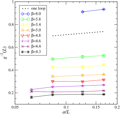
We compare to the one-loop formula,
| (19) |
where , by plotting Eq. (19) as the dotted line in the figure. At we find that the coupling runs with the slope of the one-loop result, but runs more slowly at all stronger bare couplings. For each , the change in the coupling over the widest range of for which we have data is never more than about 15 per cent. This should be compared to the case of QCD with , where is more than twice as large and where in nonperturbative studies the coupling always runs faster than perturbation theory predicts (see Ref. DellaMorte:2004bc ). In an ordinary QCD simulation, one wishes to simulate at bare parameter values where the theory is weakly interacting at short distance, so that one can use perturbation theory to match lattice-regulated matrix elements to their continuum-regulated counterparts. One makes the lattice large enough so that the system becomes strongly interacting at long distance, so that the simulation captures the physics of confinement. Satisfying both conditions does not seem to be possible for sextet QCD.
Note also that there does not seem to be any value of the bare coupling at which clearly decreases as increases. This means that we cannot argue for the existence of an IRFP.
From Fig. 4 we derive finite-lattice approximations to the step-scaling function (SSF), conventionally defined by comparing measured on two lattices, viz.,
| (20) |
where and is the scale factor between the two lattices. Thus is the change in the SF coupling when the lattice IR scale is changed by a factor of . For scale factor we can compare lattices with and as well as lattices with and ; for we compare and and also and . We plot , which parallels the usual continuum beta function,444For instance, a negative value for means asymptotic freedom. for these scale factors in Figs. 5 and 6.
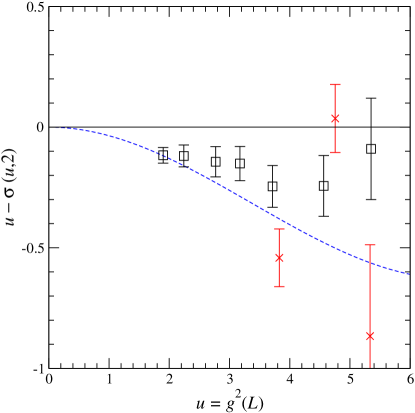
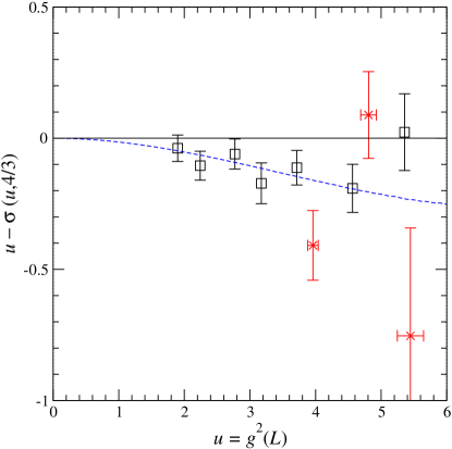
The curves come from integrating the two-loop beta function from to [cf. Eq. (18)].
We see in Fig. 5 that the SSF from the comparison reflects running that is consistently slower than the integrated two-loop beta function. It is possible that the rightmost point indicates a fixed point (where we would have ), but the error bar is large; also this point was measured in a metastable state, so its interpretation is unclear. As for the SSF, the most we can say is that it is not inconsistent with that from the smaller lattices. The SSF for scale factor (Fig. 6) tells a similar story.
In order to connect to our earlier work Shamir:2008pb on the thin-link lattice theory (on smaller lattices) we also plot the discrete beta function (DBF) as defined there,555The definition in Ref. Shamir:2008pb included a factor of [see Eq. (12) above] which we drop here.
| (21) |
where (Fig. 7.)
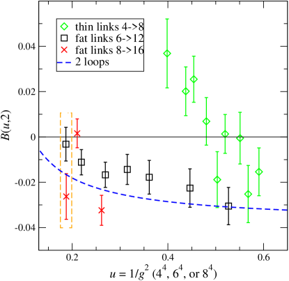
Again we note that the fat-link results show running that is slower than two-loop perturbation theory, but no solid evidence for an IRFP. In fact they rule out the fixed point found in the thin-link theory (on smaller lattices) at .
The apparent linearity of the data in Fig. 4 suggests trying to collapse all the DBF’s onto each other by plotting the ratio
| (22) |
combining data for all available scale factors on one graph. gives the beta function for when in the continuum limit . This is shown in Fig. 8.
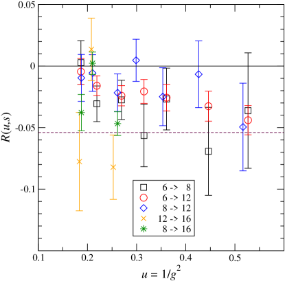
While, again, the data show slower running than the two-loop prediction, the scatter and the error bars pretty much preclude any ambitious further analysis.
A complete analysis of the data would involve taking the limit. In principle, doing this on the weak coupling side of the phase transition would produce a result that is free of lattice discretization errors. Fig. 8 shows that the scatter in from different values of is at least as large as the statistical fluctuations in the individual points. A fit to , for example, would just produce noise. We are defeated by the slow intrinsic running of the coupling. Nonetheless, we can at least make two plain statements:
-
•
The IRFP observed in Ref. Shamir:2008pb is ruled out.
-
•
The SF coupling runs slowly over its observed range. This slow running permits an easy and unambiguous measurement of the mass anomalous dimension as a function of the bare parameters or, equivalently, of the SF coupling . This is the subject of the next section.
V Mass anomalous dimension
After the discussion of the running gauge coupling, our result for the mass anomalous dimension is more definite: is never larger in magnitude than about 0.6. This confirms the previous, noisy results of Ref. DeGrand:2009hu . It suggests that, regardless of the existence of a zero of the beta function, this theory may not furnish a phenomenologically interesting model of walking technicolor.
We extract the anomalous dimension of from the scaling of [Eq. (14)] between systems rescaled as . We define the (continuum) mass step scaling function Sint:1998iq ; Capitani:1998mq ; DellaMorte:2005kg ; Bursa:2009we as
| (23) |
It is related to the mass anomalous dimension via
| (24) |
Equation (24) is actually too complicated for our needs. For any bare coupling , the SF coupling runs so slowly that we can replace Eq. (24) by
| (25) |
| 5.8 | 0.2696(16) | 0.2509(12) | 0.2248(18) | – |
| 5.4 | 0.2606(19) | 0.2333(14) | 0.2102(17) | – |
| 5.0 | 0.2398(19) | 0.2318(15) | 0.1839(14) | – |
| 4.8 | 0.2246(23) | 0.1981(15) | 0.1716(10) | – |
| 4.6 | 0.2127(14) | 0.1808(16) | 0.1518(14) | 0.1340(6) |
| 4.4 | 0.1888(18) | 0.1631(16) | 0.1311(13) | 0.1163(13) |
| 4.3 | 0.1777(17) | 0.1516(17) | 0.1247(15) | 0.1063(10) |
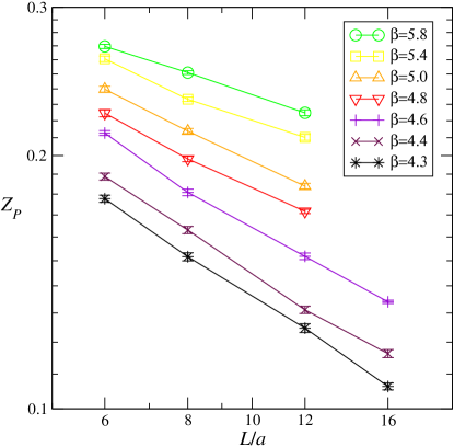
As can be seen in the figure, the -dependence of is very close to linear on a log–log plot at all values of . This is a consequence of the slow running of the coupling constant. The theory is “conformal for all practical purposes” over the range of ’s that are accessible at any single value of . The slopes of the curves allow us to read off since the simplified Eq. (25) implies
| (26) |
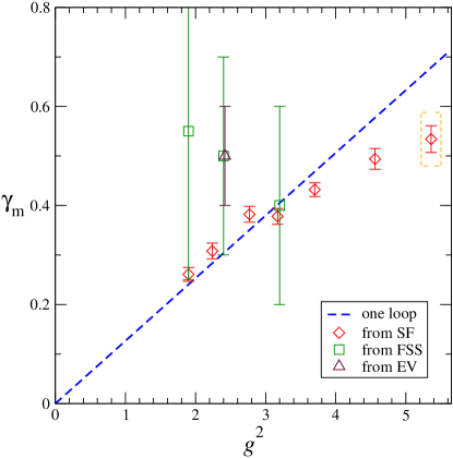
We thus fit straight lines to the data in Fig. 9, keeping only the three largest volumes at each . The result of the analysis is shown in Fig. 10, a plot of versus the SF coupling . We use for each bare coupling ; since varies so little, this gives a good first approximation. We compare to the one-loop perturbative expectation, . It can be seen that the numerical results follow the perturbative line closely until they deviate downward at the strongest couplings. The agreement with Ref. DeGrand:2009hu is gratifying, as is the much smaller uncertainty obtained with the present method.
To study finite-lattice effects we define the lattice approximation to the step scaling function (23),
| (27) |
such that
| (28) |
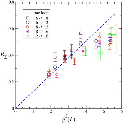
We form the ratios of Eq. (27) from the data in Table 3. The rescaled quantities
| (29) |
give directly as in the continuum limit. They are shown for two bare couplings, and 4.6, in Fig. 11. At these couplings, we have data for , 8, 12, and 16 and so we can form two combinations each with and . We also plot the analogous result for the pair . While there does appear to be some cutoff () dependence, no possible extrapolation to can push much above 0.6. We follow up this figure with a compilation of , plotted against for many pairs of , in Fig. 12.


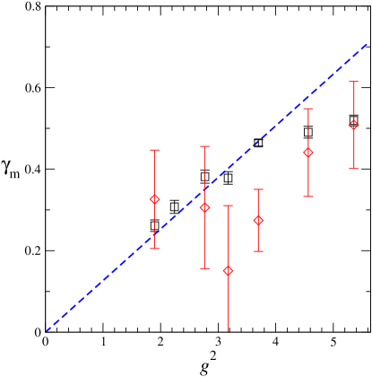
We can use all the data to derive by fitting at each to the form
| (30) |
The fit involves three parameters if is kept, two if it is discarded. Again, at any particular value of the bare coupling, the spread of is so small as to be irrelevant in any plots. Table 4 and Fig. 13 show the results of two-parameter and three parameter fits to all (three or four) data points at each value. Fitting all the data at one value to the three-parameter form produces results that are basically identical to those obtained if values of are themselves used to approximate as above, whereupon is then fit to . The data do not really allow us to say much, especially when we only have three ’s per value; nonetheless the figure does confirm that never rises above 0.6. Lattice spacing artifacts will not alter our result.
| ’s kept | |||
|---|---|---|---|
| 5.8 | 8, 12 | 0.271(23) | 0 |
| 6, 8, 12 | 0.261(14) | 0.29 | |
| 5.4 | 8, 12 | 0.257(25) | 0 |
| 6, 8, 12 | 0.308(15) | 7.12 | |
| 5.0 | 8, 12 | 0.372(25) | 0 |
| 6, 8, 12 | 0.382(16) | 0.26 | |
| 4.8 | 8, 12 | 0.353(23) | 0 |
| 6, 8, 12 | 0.378(15) | 2.04 | |
| 4.6 | 6, 8, 12 | 0.432(14) | 0.0003 |
| 6, 8, 12, 16 | 0.464(8) | 7.3 | |
| 4.4 | 6, 8, 12 | 0.494(21) | 2.7 |
| 6, 8, 12, 16 | 0.491(14) | 2.7 | |
| 4.3 | 6, 8, 12 | 0.512(20) | 0.77 |
| 6, 8, 12, 16 | 0.519(13) | 0.98 |
VI Summary and conclusions
Our system exhibits two phases, a weak-coupling phase which is nonconfining and chirally restored, and a strong-coupling phase which is confining. The AWI quark mass does not vanish in the confining phase, so we cannot perform a Schrödinger functional study there (except in a metastable state). In the weak coupling phase, we find that the SF coupling runs more slowly than predicted by two-loop perturbation theory over the entire domain of couplings accessible to analysis.
The location of the fixed point reported in our earlier paper is not confirmed. The present simulation has an improved lattice discretization and larger simulation volumes. We did not observe an IRFP, nor did we rule one out. We did not observe a positive beta function anywhere.
We studied the first-order phase boundary in some detail. In order to ascertain the relevance of this transition to continuum physics one has to study its location and strength on yet larger lattices. Moreover, the location of this transition almost certainly depends on the particular choice of bare action. An obvious question is whether one can devise lattice discretizations that push the transition to larger values of the SF coupling. Then it is possible that the extension of the beta function to larger couplings will reveal a fixed point.
Of other gauge theories similar to ours, the one with the most similar result is the SU(2) gauge theory with fermions in the adjoint representation—a candidate for “minimal walking technicolor” (MWT) Bursa:2009we ; DelDebbio:2010hu ; DelDebbio:2010hx ; Catterall:2007yx ; Catterall:2008qk ; Hietanen:2008mr ; Hietanen:2009az ; Catterall:2009sb . Its SF gauge coupling runs slowly, and evidence for a zero is ambiguous. It has a small, nearly perturbative mass anomalous dimension. In these studies also Wilson fermions were used. There is a first-order transition as is varied in strong coupling, but, in contrast to our results, this line ends in a critical point Catterall:2008qk ; Hietanen:2008mr . The connection of what is evidently a bulk transition to the finite-temperature phase transition is unclear. Nonetheless, the critical point itself is a sign of interesting structure along the line. The latter is bounded by IR-repulsive fixed points at zero coupling (asymptotic freedom) and at strong coupling (the critical point), which may indicate that it is in the basin of attraction of an IR-attractive fixed point and hence that it constitutes a conformal phase. We emphasize that, in contrast, our first-order transition at continues smoothly into the first-order finite-temperature transition at without any sign of a critical point at the intersection with the line.
The other class of slowly running theories is SU(3) gauge theory with flavors of light fermions in the fundamental representation. The earliest study of the phase diagram using Wilson fermions is that of Iwasaki et. al Iwasaki:1991mr ; Iwasaki:2003de . The authors found, for , that “the massless quark line exists only in the deconfined phase.” Recent simulations Nagai:2009ip in strong coupling for SU(2) and SU(3) gauge groups confirm this picture, with first order behavior (i.e., no where ) appearing at for SU(2) and in the range 6–8 for SU(3). Simulations with Wilson fermion flavors Yamada:2010wd also produce a first order transition in strong coupling.
Kogut and Sinclair Kogut:2010cz have studied the SU(3) gauge theory with sextet fermions and reached conclusions rather different from ours. They report the existence of two finite-temperature transitions, a chiral and a confinement transition, at very different bare gauge couplings, implying both dramatic scale separation and non-conformal physics. That study was done with unimproved staggered fermions and the usual square-root prescription. Away from the continuum limit, this prescription is known to induce non-localities; equivalently, the number of quark species is not well defined.666For a recent review, see Ref. Golterman:2008gt . It is important to monitor the magnitude of taste violation carefully in such calculations. Badly broken taste symmetry would mean that the theory under study has fewer effective massless flavors, which would bias the result towards confinement rather than conformality.
Returning to the present study, we note again that the slow running of the gauge coupling constant allows an inexpensive and accurate measurement of the mass anomalous dimension . This measurement confirms, and considerably improves on, the calculation of Ref. DeGrand:2009hu . is small, never greater than 0.6 in the coupling region where we can measure it.
The small value of in this theory presents a challenge for technicolor phenomenology. Even if sextet QCD is not phenomenologically viable, however, it is characterized by a coupling constant that evolves very slowly with scale. Such systems are theoretically interesting in their own right.
Acknowledgements.
We thank S. Chivukula, P. Damgaard, A. Hasenfratz, D. Kaplan, A. Nelson, and E. Simmons for discussions and correspondence. T. D. is grateful for the hospitality of the Niels Bohr International Academy during part of the time he carried out this research. B. S. and Y. S. thank the University of Colorado for hospitality. This work was supported in part by the Israel Science Foundation under grants no. 173/05 and no. 423/09 and by the US Department of Energy. This research was also supported in part by the National Science Foundation through TeraGrid resources provided by the University of Texas under grants no. TG-PHY080042 and no. TG-PHY090023. Further computations were done on clusters at the University of Colorado and at Tel Aviv University. Our computer code is based on the publicly available package of the MILC collaboration MILC . The code for hypercubic smearing was adapted from a program written by A. Hasenfratz, R. Hoffmann and S. Schaefer Hasenfratz:2008ce .*
Appendix A Illustrations of the Strong Coupling Transition


In this appendix we present data supporting the location of the first-order phase transitions for and 8, as well as determinations of where the boundaries cross the curve. (We denote the crossing points by , for and .)
First we show data for the AWI quark mass (Fig. 14) and plaquette average (Fig. 15) from simulations with SF boundary conditions. Each curve shows the variation with for a given , as is swept across the phase boundary at . The first-order transition is evident in each curve, as is the fact that the discontinuity nowhere tends to zero: There is no critical point anywhere.


In Fig. 14 we see that the condition can be used to define for , where while . Thus the phase boundary and the curve are distinct for , as seen in Figs. 1 and 2. For we find that crosses zero discontinuously, and thus there is no curve here. (The data shown here refer to equilibrium states only; the metastable extension of the curve to the left of cannot be seen.)

Since the variation of is of great importance, we devote some effort to interpolating to find its intersection with the curve. In Fig. 16 we plot the difference vs. , where is determined in the deconfined phase. (Where this quantity is positive, the phase boundary lies above the curve; the AWI quark mass in the deconfined phase at the phase boundary is negative, and the point lies in a metastable phase.) The curves in the figure are quadratic fits. Inverting them to find , the point where the transition crosses the curve, we find for (with dof) and 4.383(10) for (with ). The difference is then , to be compared to the prediction of 0.08 from Eq. (18). These results are stable under variation in the number of points used in the fit: For example, quadratic fits to the three points at , 4.35 and 4.4 give 4.308(6) and 4.376(15) for , respectively.
References
- (1) C. T. Hill and E. H. Simmons, “Strong dynamics and electroweak symmetry breaking,” Phys. Rept. 381, 235 (2003) [Erratum-ibid. 390, 553 (2004)] [arXiv:hep-ph/0203079];
- (2) H. Georgi, “Unparticle Physics,” Phys. Rev. Lett. 98, 221601 (2007) [arXiv:hep-ph/0703260]; “Another Odd Thing About Unparticle Physics,” Phys. Lett. B 650, 275 (2007) [arXiv:0704.2457 [hep-ph]].
- (3) For reviews see E. Pallante, “Strongly and slightly flavored gauge theories,” arXiv:0912.5188 [hep-lat]; G. T. Fleming, “Strong Interactions for the LHC,” PoS LATTICE2008, 021 (2008) [arXiv:0812.2035 [hep-lat]].
- (4) W. E. Caswell, “Asymptotic behavior of nonabelian gauge theories to two loop order,” Phys. Rev. Lett. 33, 244 (1974).
- (5) T. Banks and A. Zaks, “On the phase structure of vector-like gauge theories with massless fermions,” Nucl. Phys. B 196, 189 (1982).
- (6) B. Holdom, “Raising The Sideways Scale,” Phys. Rev. D 24, 1441 (1981).
- (7) K. Yamawaki, M. Bando and K. i. Matumoto, Phys. Rev. Lett. 56, 1335 (1986).
- (8) T. Appelquist, J. Terning and L. C. R. Wijewardhana, “Postmodern technicolor,” Phys. Rev. Lett. 79, 2767 (1997) [arXiv:hep-ph/9706238].
- (9) R. S. Chivukula and E. H. Simmons, “Condensate enhancement and -meson mixing in technicolor theories,” arXiv:1005.5727 [hep-lat].
- (10) A. E. Nelson, “Lattice calculations for physics beyond the standard model,” PoS LAT2006, 016 (2006).
- (11) F. Sannino and K. Tuominen, “Orientifold theory dynamics and symmetry breaking,” Phys. Rev. D 71, 051901 (2005) [arXiv:hep-ph/0405209].
- (12) D. K. Hong, S. D. H. Hsu and F. Sannino, “Composite Higgs from higher representations,” Phys. Lett. B 597, 89 (2004) [arXiv:hep-ph/0406200].
- (13) D. D. Dietrich, F. Sannino and K. Tuominen, “Light composite Higgs from higher representations versus electroweak precision measurements: Predictions for LHC,” Phys. Rev. D 72, 055001 (2005) [arXiv:hep-ph/0505059].
- (14) A. Belyaev, R. Foadi, M. T. Frandsen, M. Jarvinen, F. Sannino and A. Pukhov, “Technicolor walks at the LHC,” Phys. Rev. D 79, 035006 (2009) [arXiv:0809.0793 [hep-ph]].
- (15) Y. Shamir, B. Svetitsky and T. DeGrand, “Zero of the discrete beta function in SU(3) lattice gauge theory with color sextet fermions,” Phys. Rev. D 78, 031502 (2008) [arXiv:0803.1707 [hep-lat]].
- (16) T. DeGrand, Y. Shamir and B. Svetitsky, “Phase structure of SU(3) gauge theory with two flavors of symmetric-representation fermions,” Phys. Rev. D 79, 034501 (2009) [arXiv:0812.1427 [hep-lat]].
- (17) T. DeGrand, “Finite-size scaling tests for SU(3) lattice gauge theory with color sextet fermions,” Phys. Rev. D 80, 114507 (2009) [arXiv:0910.3072 [hep-lat]].
- (18) Z. Fodor, K. Holland, J. Kuti, D. Nógradi and C. Schroeder, “Chiral properties of SU(3) sextet fermions,” JHEP 0911, 103 (2009) [arXiv:0908.2466 [hep-lat]].
- (19) O. Machtey and B. Svetitsky, “Metastable nonconfining states in SU(3) lattice gauge theory with sextet fermions,” Phys. Rev. D 81, 014501 (2010) [arXiv:0911.0886 [hep-lat]].
- (20) J. B. Kogut and D. K. Sinclair, “Thermodynamics of lattice QCD with 2 flavours of colour-sextet quarks: A model of walking/conformal Technicolor,” arXiv:1002.2988 [hep-lat].
- (21) Y. Iwasaki, K. Kanaya, S. Kaya, S. Sakai and T. Yoshié, “Phase structure of lattice QCD for general number of flavors,” Phys. Rev. D 69, 014507 (2004) [arXiv:hep-lat/0309159].
- (22) B. Sheikholeslami and R. Wohlert, “Improved continuum limit lattice action for QCD with Wilson fermions,” Nucl. Phys. B 259, 572 (1985).
- (23) A. Hasenfratz, R. Hoffmann and S. Schaefer, “Hypercubic smeared links for dynamical fermions,” JHEP 0705, 029 (2007) [arXiv:hep-lat/0702028].
- (24) M. Hasenbusch, “Speeding up the Hybrid-Monte-Carlo algorithm for dynamical fermions,” Phys. Lett. B 519, 177 (2001) [arXiv:hep-lat/0107019].
- (25) C. Urbach, K. Jansen, A. Shindler and U. Wenger, “HMC algorithm with multiple time scale integration and mass preconditioning,” Comput. Phys. Commun. 174, 87 (2006) [arXiv:hep-lat/0506011].
- (26) T. Takaishi and P. de Forcrand, “Testing and tuning new symplectic integrators for hybrid Monte Carlo algorithm in lattice QCD,” Phys. Rev. E 73, 036706 (2006) [arXiv:hep-lat/0505020].
- (27) R. Hoffmann, A. Hasenfratz and S. Schaefer, “Non-perturbative improvement of nHYP smeared Wilson fermions,” PoS LAT2007, 104 (2007) [arXiv:0710.0471 [hep-lat]].
- (28) Y. Shamir, B. Svetitsky, and E. Yurkovsky, in preparation.
- (29) See the tables in T. A. DeGrand, A. Hasenfratz and T. G. Kovacs, “Improving the chiral properties of lattice fermions,” Phys. Rev. D 67, 054501 (2003) [arXiv:hep-lat/0211006]. For nonperturbative determinations (with fundamental representation fermions), see Ref. Hasenfratz:2008ce .
- (30) M. Lüscher, R. Narayanan, P. Weisz and U. Wolff, Nucl. Phys. B 384, 168 (1992) [arXiv:hep-lat/9207009].
- (31) M. Lüscher, R. Sommer, P. Weisz and U. Wolff, “A precise determination of the running coupling in the SU(3) Yang-Mills theory,” Nucl. Phys. B 413, 481 (1994) [arXiv:hep-lat/9309005].
- (32) S. Sint and R. Sommer, “The running coupling from the QCD Schrödinger functional: A one loop analysis,” Nucl. Phys. B 465, 71 (1996) [arXiv:hep-lat/9508012].
- (33) K. Jansen and R. Sommer [ALPHA collaboration], “O() improvement of lattice QCD with two flavors of Wilson quarks,” Nucl. Phys. B 530, 185 (1998) [Erratum-ibid. B 643, 517 (2002)] [arXiv:hep-lat/9803017].
- (34) M. Della Morte et al. [ALPHA Collaboration], “Computation of the strong coupling in QCD with two dynamical flavours,” Nucl. Phys. B 713, 378 (2005) [arXiv:hep-lat/0411025].
- (35) S. Sint and P. Weisz [ALPHA collaboration], “The running quark mass in the SF scheme and its two-loop anomalous dimension,” Nucl. Phys. B 545, 529 (1999) [arXiv:hep-lat/9808013].
- (36) S. Capitani, M. Lüscher, R. Sommer and H. Wittig [ALPHA Collaboration], “Non-perturbative quark mass renormalization in quenched lattice QCD,” Nucl. Phys. B 544, 669 (1999) [arXiv:hep-lat/9810063].
- (37) M. Della Morte et al. [ALPHA Collaboration], “Non-perturbative quark mass renormalization in two-flavor QCD,” Nucl. Phys. B 729, 117 (2005) [arXiv:hep-lat/0507035].
- (38) F. Bursa, L. Del Debbio, L. Keegan, C. Pica and T. Pickup, “Mass anomalous dimension in SU(2) with two adjoint fermions,” Phys. Rev. D 81, 014505 (2010) [arXiv:0910.4535 [hep-ph]].
- (39) J. L. Cardy, Scaling and Renormalization in Statistical Physics, (Cambridge, UK: Univ. Pr., 1996), 238 p.
- (40) A. D. Kennedy, J. Kuti, S. Meyer and B. J. Pendleton, “Where is the continuum in lattice quantum chromodynamics?,” Phys. Rev. Lett. 54, 87 (1985).
- (41) S. A. Gottlieb et al., “The deconfining phase transition and the continuum limit of lattice quantum chromodynamics,” Phys. Rev. Lett. 55, 1958 (1985).
- (42) F. Farchioni et al., “Twisted mass quarks and the phase structure of lattice QCD,” Eur. Phys. J. C 39, 421 (2005) [arXiv:hep-lat/0406039].
- (43) S. Catterall and F. Sannino, “Minimal walking on the lattice,” Phys. Rev. D 76, 034504 (2007) [arXiv:0705.1664 [hep-lat]].
- (44) S. Catterall, J. Giedt, F. Sannino and J. Schneible, “Phase diagram of SU(2) with 2 flavors of dynamical adjoint quarks,” JHEP 0811, 009 (2008) [arXiv:0807.0792 [hep-lat]].
- (45) A. J. Hietanen, J. Rantaharju, K. Rummukainen and K. Tuominen, “Spectrum of SU(2) lattice gauge theory with two adjoint Dirac flavours,” JHEP 0905, 025 (2009) [arXiv:0812.1467 [hep-lat]].
- (46) A. J. Hietanen, K. Rummukainen and K. Tuominen, “Evolution of the coupling constant in SU(2) lattice gauge theory with two adjoint fermions,” Phys. Rev. D 80, 094504 (2009) [arXiv:0904.0864 [hep-lat]].
- (47) S. Catterall, J. Giedt, F. Sannino and J. Schneible, “Probes of nearly conformal behavior in lattice simulations of minimal walking technicolor,” arXiv:0910.4387 [hep-lat].
- (48) L. Del Debbio, B. Lucini, A. Patella, C. Pica and A. Rago, “Mesonic spectroscopy of Minimal Walking Technicolor,” arXiv:1004.3197 [hep-lat].
- (49) L. Del Debbio, B. Lucini, A. Patella, C. Pica and A. Rago, “The infrared dynamics of Minimal Walking Technicolor,” arXiv:1004.3206 [hep-lat].
- (50) Y. Iwasaki, K. Kanaya, S. Sakai and T. Yoshié, “Quark confinement and number of flavors in strong coupling lattice QCD,” Phys. Rev. Lett. 69, 21 (1992).
- (51) K. Nagai, G. Carrillo-Ruiz, G. Koleva and R. Lewis, “Exploration of SU() gauge theory with many Wilson fermions at strong coupling,” Phys. Rev. D 80, 074508 (2009) [arXiv:0908.0166 [hep-lat]].
- (52) N. Yamada et al., “Study of the running coupling constant in 10-flavor QCD with the Schrödinger functional method,” arXiv:1003.3288 [hep-lat];
- (53) M. Golterman, PoS CONFINEMENT8, 014 (2008) [arXiv:0812.3110 [hep-ph]].
- (54) http://www.physics.utah.edu/detar/milc/
- (55) A. Hasenfratz, R. Hoffmann and S. Schaefer, “Low energy chiral constants from epsilon-regime simulations with improved Wilson fermions,” Phys. Rev. D 78, 054511 (2008) [arXiv:0806.4586 [hep-lat]].