Comparison of the experimental data for the Casimir pressure with the Lifshitz theory at zero temperature

Abstract

We perform detailed comparison of the experimental data of the experiment on the determination of the Casimir pressure between two parallel Au plates with the theoretical values computed using the Lifshitz formula at zero temperature. Computations are done using the optical data for the complex index of refraction of Au extrapolated to low frequencies by means of the Drude model with both most often used and other suggested Drude parameters. It is shown that the experimental data exclude the Lifshitz formula at zero temperature at a 70% confidence level if the Drude model with most often used values of the parameters is employed. If other values of the Drude parameters are used, the Lifshitz formula at zero frequency is experimentally excluded at a 95% confidence level. The Lifshitz formula at zero temperature combined with the generalized plasma-like model with most often used value of the plasma frequency is shown to be experimentally consistent. We propose a decisive experiment which will shed additional light on the role of relaxation properties of conduction electrons in the Casimir effect.

I Introduction

There is an increasing interest in the Casimir effect 1 in the recent literature connected with numerous multidisciplinary applications in both fundamental and applied science (see monograph 2 for a modern overview of the subject). The Casimir force acting between two closely spaced uncharged material bodies is connected with the existence of zero-point and thermal fluctuations of the electromagnetic field. Keeping in mind that in some sense the vacuum is the most fundamental quantum state, the role of the Casimir force in many diverse areas ranging from elementary particles and gravitation to atomic physics, condensed matter physics and nanotechnology becomes clear. Over a long period of time the experimental investigation of the Casimir effect has progressed only slowly because the related forces and energies are very small and their observation requires special conditions which are hard to achieve. During the last 12 years, however, about 25 experiments measuring the Casimir force have been performed using new possibilities suggested by modern laboratory techniques (the review 3 describes all recent experiments and related theory).

It is well known that the most fundamental theoretical description of the van der Waals and Casimir forces acting between two material bodies is given by the Lifshitz theory 4 ; 5 ; 6 (recall that in this case the Casimir force is nothing but the retarded van der Waals force). The Lifshitz theory was originally formulated for two semispaces separated by a gap. Recently far-reaching generalizations of the Lifshitz theory have been proposed allowing calculation of the Casimir force between arbitrarily shaped bodies (see, for instance, Refs. 2 ; 7 ; 8 ; 9 ; 10 ; 11 ; 12 ; 13 ; 14 ; 15 ). In the Lifshitz theory and its generalizations the Casimir energy and force are expressed in terms of reflection amplitudes describing reflection of the electromagnetic oscillations on the boundary surfaces. If the spatial dispersion of material bodies can be neglected, the reflection amplitudes in turn are expressed using the dielectric permittivity depending on the frequency $\omega$. This is in fact the basic quantity in the Lifshitz theory which should be known to calculate the Casimir energy (free energy) and the Casimir force.

The comparison of the experimental data with the Lifshitz theory at nonzero temperature has revealed a puzzle which remains unresolved to the present day 3 . Some authors 16 ; 17 ; 18 (see complete set of references in review 3 ) consider most natural the suggestion to substitute in the Lifshitz formula the full dielectric permittivity taking into account all physical processes really occurring at the corresponding frequencies. This leads to the use of dielectric permittivity containing the first order pole at $\omega=0$ due to the role of conduction electrons. The respective behavior of the dielectric permittivity at low frequencies is usually described by the Drude model. However, the experimental data of several experiments performed at nonzero temperature with metallic 19 ; 20 ; 21 ; 22 , semiconductor 23 ; 24 and dielectric 25 ; 26 test bodies are inconsistent with the theoretical predictions of the Lifshitz theory obtained using this suggestion. Different attempts on how to resolve the puzzle of the thermal Casimir force, including the question of reliability of the data, were discussed 27 (see also in Secs. II and III below).

The use of the Lifshitz formula at zero temperature $T=0$ is one of the widespread approaches to the comparison of measurement data with theory in Casimir physics 28 ; 29 ; 30 ; 31 . This is usually justified by stating that at small separations between the test bodies the corrections to the Casimir force due to nonzero temperature are insignificant. It should be noted that the role of nonzero temperature in the Lifshitz formula is twofold: in the discreteness of the imaginary frequencies at $T\neq 0$ and in the explicit dependence of the dielectric permittivity on $T$. What is commonly referred to as “the Lifshitz formula at zero temperature”, takes into account only the first factor. This means that the integration with respect to a continuous frequency is performed instead of summation over the discrete Matsubara frequencies. In so doing the second factor is disregarded, i.e., the dielectric permittivity, as measured at room temperature, is preserved. The “hybrid” character of such kind of “zero-temperature” formula was investigated 32 . Specifically, it was shown that respective “zero-temperature” Casimir energy, even at short separations, can deviate from the Casimir free energy computed at room temperature by several percents. Nevertheless it is rather common to believe 33 that the Lifshitz formula at zero temperature “gives a dominant contribution at small separations ($<1\,\mu$m at room temperature) between the bodies and was readily confirmed experimentally with good accuracy…”.

In this paper we perform the detailed comparison of the experimental data on an indirect measurement of the Casimir pressure between two parallel plates 21 ; 22 with the Lifshitz formula for the Casimir pressure at zero temperature. This comparison is performed using the tabulated 34 optical data for Au extrapolated to low frequencies by means of the Drude model with most often used Drude parameters 39 and with other Drude parameters, as suggested, e.g., in Ref. 35 . Our comparison shows that the experimental data exclude the Lifshitz formula at zero temperature, which uses the tabulated optical data extrapolated to low frequencies with the help of most often used Drude parameters, at a 70% confidence level over a wide separation region. The zero-temperature Lifshitz formula using other Drude parameters is excluded by the data at a 95% confidence level. According to our results, if the experiment is performed at room temperature, the Lifshitz formula also at room temperature should be used to make a comparison between the data and the theory. We discuss a recent suggestion 37 on how to avoid the use of ad hoc extrapolations of the optical data outside the frequency region where they were measured. This suggestion is based on some properties of analytic functions but meets difficulties in practical realization. We also consider the Lifshitz formula at zero temperature using the generalized plasma-like model 2 ; 3 ; 36 , which disregards relaxation properties of conduction electrons, and compare the computational results with the same experimental data. It was shown that in this case the data are consistent with the theory employing the most often used value of the plasma frequency. This is explained by the fact that the generalized plasma-like model at separations below $1\,\mu$m leads to approximately the same results irrespective of whether the Lifshitz formula at zero or nonzero temperature is used. We also propose a new experiment which can shed additional light on the role of relaxation properties of conduction electrons in the Casimir effect.

The paper is organized as follows. In Sec. II we compare the experimental data 21 ; 22 with the zero-temperature Lifshitz formula which utilizes the extrapolation of the optical data by the Drude model with most often used parameters. In Sec. III the same data are compared with the same formula, but with other Drude parameters. The possibility on how to determine the dielectric permittivity along the imaginary frequency axis using only the measured optical data is discussed in Sec. IV. Section V is devoted to the comparison of the experimental data with the Lifshitz formula at zero temperature combined with the generalized plasma-like model. In Sec. VI the reader will find our conclusions and discussion including the proposal of new decisive experiment.

II Comparison of the experimental data with theory
using conventional extrapolation of the optical data by the Drude model

Here and below we use the experimental data of the experiment on an indirect measurement of the Casimir pressure between two parallel plates by means of micromachined oscillator 21 ; 22 . This experiment used the configuration of a Au-coated sphere of $150\,\mu$m radius above a Au-coated plate that could rotate about the rotation axis. During the measurements, the separation between the sphere and the plate was varied harmonically at the resonant frequency of the oscillator. The immediately measured quantity was the shift in this frequency due to the Casimir force acting between the sphere and the plate. Using the proximity force approximation 2 ; 3 ; 38 , the shift of the resonant frequency of the oscillator was recalculated into the equivalent Casimir pressure in the configuration of two parallel plates made of Au. The pressure was determined as a function of separation over the separation region from 160 to 750 nm. The absolute error in the measurement of separation distances $a$ was determined to be $\Delta a=0.6\,$nm at a 95% confidence level. The absolute error in the determination of the Casimir pressure was also determined at a 95% confidence level and found to be separation-dependent. The respective relative error increases from approximately 0.2% at $a=160\,$nm to 9% at $a=750\,$nm. It was shown that in this experiment the total experimental error is completely determined by the systematic error leaving the random error negligibly small, as it should be in precise experiments of metrological quality (details of the measurements, calculations and error analysis can be found in Refs. 2 ; 3 ; 21 ; 22 ).

According to our aim, the theoretical Casimir pressure between smooth parallel plates is computed using the Lifshitz formula at zero temperature

$$P(a)=-\frac{\hbar}{2\pi^{2}}\int_{0}^{\infty}d\xi\int_{0}^{\infty}k_{\bot}dk_{\bot}q\sum\limits_{\alpha}\left[\frac{e^{2aq}}{r_{\alpha}^{2}(i\xi,k_{\bot})}-1\right]^{-1}.$$ (1)

Here, $\omega=i\xi$, $k_{\bot}$ is the projection of the wave vector onto the plane of the plates, $\alpha$ denotes the transverse magnetic (TM) and transverse electric (TE) polarizations of the electromagnetic field, and $q=(k_{\bot}^{2}+\xi^{2}/c^{2})^{1/2}$. The respective reflection coefficients are

$$r_{\rm TM}(i\xi,k_{\bot})=\frac{\varepsilon(i\xi)q-k}{\varepsilon(i\xi)q+k},$$

$$r_{\rm TE}(i\xi,k_{\bot})=\frac{q-k}{q+k},$$ (2)

where $k=[k_{\bot}^{2}+\varepsilon(i\xi)\xi^{2}/c^{2}]^{1/2}$ and $\varepsilon(i\xi)$ is the dielectric permittivity of the material calculated along the imaginary frequency axis.

We have performed computations by Eqs. (1) and (2) within the experimental separation region from 160 to 750 nm. The dielectric permittivity of Au along the imaginary frequency axis was found by means of the Kramers-Kronig relation 2 which assumes that $\varepsilon(\omega)$ is regular or has a first-order pole at $\omega=0$:

$$\varepsilon(i\xi)=1+\frac{2}{\pi}\int_{0}^{\infty}\frac{\omega\,{\rm Im}\,\varepsilon(\omega)}{\xi^{2}+\omega^{2}}\,d\omega.$$ (3)

This was done using the tabulated optical data 34 for the imaginary part of the dielectric permittivity, ${\rm Im}\,\varepsilon(\omega)$, measured in the frequency region from 0.125 to $10^{4}\,$eV and extrapolated to lower frequencies by means of the Drude model

$$\varepsilon(i\xi)=1+\frac{\omega_{p}^{2}}{\xi(\xi+\gamma)}.$$ (4)

The values of the plasma frequency $\omega_{p}$ and relaxation parameter $\gamma$ were determined 22 from the measurements of resisitivity of the used Au films as a function of temperature. These values ($\omega_{p}=8.9\,$eV and $\gamma=0.0357\,$eV) are very close to the values 34 ; 39 $\omega_{p}=9.0\,$eV and $\gamma=0.035\,$eV most often used in numerous calculations of the Casimir force between Au surfaces made by different authors (see review 2 ; 3 ). It was not needed to use any extrapolation of the optical data to higher frequencies.

The influence of surface roughness was taken into account in a nonmultiplicative way using the method of geometrical averaging 2 ; 3 ; 20 ; 22 . According to this method the theoretical Casimir pressures between the rough plates were calculated as

$$P^{\rm theor}(a)=\sum\limits_{i=1}^{N_{p}}\sum\limits_{j=1}^{N_{s}}v_{j}^{(s)}v_{i}^{(p)}P(a+H_{s}+H_{p}-h_{j}^{(s)}-h_{i}^{(p)}).$$ (5)

Here, the surface topography of the plate (sphere) is approximately characterized by $N_{p}$ ($N_{s}$) pairs $(v_{i}^{(p)},h_{i}^{(p)})$ [$(v_{j}^{(s)},h_{j}^{(s)})$], where $v_{i}^{(p)}$ ($v_{j}^{(s)}$) is the fraction of the surface area with height $h_{i}^{(p)}$ ($h_{j}^{(s)}$). These data obtained 20 from atomic force microscope scans allow one to determine the zero-roughness levels $H_{p}$ ($H_{s}$) relative to which the mean values of roughness profiles are equal to zero

$$\sum\limits_{i=1}^{N_{p}}(H_{p}-h_{i}^{(p)})v_{i}^{(p)}=0,\quad\sum\limits_{j=1}^{N_{s}}(H_{s}-h_{j}^{(s)})v_{j}^{(s)}=0.$$ (6)

Now we compare the computational results for the Casimir pressure at zero temperature, $P^{\rm theor}(a)$, with the experimental data 22 . In Fig. 1(a) the computational results at separations from 350 to 400 nm are shown as bands in between the two solid lines. The width of a theoretical band is determined by the total theoretical error of about 0.5% found at a 95% confidence level 20 . This includes errors due to uncertainty of the optical data 34 , contribution of patch potentials, and diffraction-type contribution to the effect of surface roughness which is not taken into account by the method of geometrical averaging (see details 20 ). The contribution of patch potentials due to grains of polycrystal Au films was estimated 20 . At the shortest separation $a=160\,$nm it was shown to be only 0.037% of the Casimir pressure, and further decreases with increasing $a$. The diffraction-type contribution to the effect of surface roughness is less 20 than 0.04% at $a=300\,$nm. Although it increases with increasing $a$, the total effect of surface roughness becomes negligibly small 20 at $a>300\,$nm. The mean experimental Casimir pressures, $\bar{P}^{\rm expt}(a)$, are shown as crosses whose arms are also determined at a 95% confidence level. All details on the measurement procedures used for measuring both the pressures and absolute separations and determination of experimental errors are presented 20 ; 21 ; 22 . Specifically, the total experimental error of pressure measurements (which is mostly determined by the systematic error) includes the error due to use of the proximity force approximation to convert the data for the frequency shift into the data for the Casimir pressure. As can be seen in Fig. 1(a), all experimental crosses lie outside of the theoretical bands, but some of the arms of the crosses touch the border lines of these bands. Thus, in the strict sense one cannot claim that the theoretical description using the Lifshitz formula at zero temperature combined with the Drude model is excluded by the data at a 95% confidence level.

Let us now perform the comparison of the experimental data with the zero-temperature theoretical results at a lower, 70%, confidence level. For this purpose we assume that both the theoretical and experimental errors are random quantities distributed uniformly (other hypothesis would lead to smaller errors at a 70% confidence level so that our approach is the most conservative 40 ). Now, to obtain the theoretical band and the arms of the experimental crosses defined at a 70% confidence level one should divide their widths in Fig. 1(a) by a factor of 0.95/0.7=1.357. The resulting comparison of experiment with theory at a 70% confidence level is presented in Fig. 1(b) within the separation region from 350 to 400 nm. The same notation as in Fig. 1(a) is used. As can be seen in Fig. 1(b), all experimental crosses are outside the theoretical band confined between the solid lines. This means that the Lifshitz theory at zero temperature employing the optical data extrapolated to zero frequency by means of the Drude model with most often used parameters is excluded by the data of the experiment 21 ; 22 at a 70% confidence level.

The obtained conclusion can be confirmed using another method for the comparison between experiment and theory based on the consideration of a confidence interval for the differences of theoretical and mean experimental Casimir pressures $P^{\rm theor}(a)-P^{\rm expt}(a)$ calculated at all experimental separations (see Refs. 2 ; 3 ; 20 ; 22 ; 41 ). At a given confidence level, such intervals $[-\Xi(a),\Xi(a)]$ are different at different separations. The confidence interval $[-\Xi_{0.95}(a),\Xi_{0.95}(a)]$ was found 22 at a 95% confidence level for the differences between predictions of the room-temperature Lifshitz theory and the experimental data 21 ; 22 . It was obtained as a combination of the total theoretical and total experimental errors. Keeping in mind that the total theoretical error is almost independent of the temperature and model of the dielectric permittivity 2 ; 3 ; 20 ; 22 , we can use the same confidence interval for the comparison between the experimental data and the theoretical results obtained using the zero-temperature Lifshitz formula.

In Fig. 2 the borders of the confidence intervals $[-\Xi_{0.95}(a),\Xi_{0.95}(a)]$ generate the two solid lines. The differences between the theoretical Casimir pressures computed using the zero-temperature Lifshitz formula and the tabulated optical data extrapolated to zero frequency are indicated as dots. As can be seen in Fig. 2, within the separation intervals $a<310\,$nm and $a>460\,$nm all dots are inside the confidence intervals, i.e., the theoretical approach used is formally consistent with the data. However, within the interval from 310 to 460 nm many dots are on the border of the confidence intervals or even outside of them. This casts some doubts on the consistency of the used theoretical approach with the data and calls for the consideration of confidence intervals at lower, 70%, confidence level. For this purpose we have investigated the distribution law of the random quantity $P^{\rm theor}(a)-P^{\rm expt}(a)$ near its mean value over the entire measurement range. We have found that to sufficient accuracy this distribution is normal. Thus, the desired half-width of the confidence interval at a 70% confidence level can be determined from the equality $\Xi_{0.95}(a)/\Xi_{0.7}(a)=2$. The obtained borders of the confidence intervals $[-\Xi_{0.7}(a),\Xi_{0.7}(a)]$ generate the two dashed lines in Fig. 2. As can be seen in this figure, over a wide separation region from 230 to 520 nm all dots lie outside the confidence intervals. This means that theoretical approach employing the zero-temperature Lifshitz formula and extrapolation of the optical data to zero frequency by means of the Drude model with most often used parameters is experimentally excluded at a 70% confidence level.

We complete this section with a brief discussion of the reliability of used experimental results and their comparison with theory. As often underlined in the literature (see, e.g., Ref. 35 ), in all performed experiments both the optical data for metallic films and the values of the Drude parameters used to extrapolate data to lower frequencies were not measured but taken from handbook 34 . It was shown 42 , however, that the variation of the optical data for Au for different samples may influence on the Casimir force on the level of 5%. The question arises whether or not this could influence the validity of the above conclusion that the Lifshitz theory at $T=0$ combined with the Drude model is experimentally excluded. First of all we recall that in the experiment 21 ; 22 the values of the Drude parameters were determined from the measurement of resistivity of the used films as a function of $T$. Recently one more measurement of the Casimir pressure by means of a micromachined oscillator was performed on a Au electroplated sample where the optical data were obtained 43 by ellipsometry in the frequency region from 1.50 to 6.25 eV. It was shown that the experimental results for the Casimir pressure in Refs. 21 ; 22 and 43 are virtually undistinguishable. The differences between the measured and tabulated optical data are very small and do not affect the computational results for the Casimir pressure 43 .

Another point that could influence the experimental results is a possible uncertainty in the electrostatic calibrations used to determine the absolute separation between the test bodies, sphere radius and some other parameters. Thus, an anomalous distance dependence of the electric force acting between an Au-coated plate and an Au-coated sphere of 30 mm radius was observed 44 . The respective contact potential was found to be dependent on separation. In experiments using micromachined oscillator the standard force-distance dependence was observed and the contact potential was measured to be constant 20 ; 21 ; 22 ; 45 ; 46 . The observed anomalous distance dependence 44 might be explained 45 by deviations of the mechanically polished and ground surface from a perfect spherical shape for lenses of centimeter-size radius. Recently the same conclusion has been made 47 for cylindrical surfaces of large radii. Notice that unexpected features of the electrostatic calibrations in the measurements of the Casimir force between metal bodies were also reported by some other authors 49 ; 50 . We emphasize, however, that in all these cases either spheres of centimeter-size radius have been used or the experiments were performed in an ambient environment (here we do not discuss the case of semiconductor test bodies where the effect of space-charge layer should be taken into account at short separations 2 ; 3 ).

The authors 44 ; 50 relate the anomalies in electrostatic calibrations observed in their experiments with large spherical lenses to possible influence of patch potentials. According to Ref. 50 , for small patches with effective area $S_{p}\ll S_{\rm eff}=2\pi Ra$, where $R$ is the sphere (lens) radius, the additional electric force arising due to the existence of patches exponentially vanishes with the increase of separation. In the opposite case of large patches satisfying the condition $S_{p}>S_{\rm eff}$, the possibility of large additional electric force arises 50 . The respective potential which minimizes the total electric force acting between a sphere of centimeter-size radius and a plate after some voltage is applied, becomes separation-dependent. As was mentioned above, in the experiments 20 ; 21 ; 22 the contact potential does not depend on separation. The investigation of the surfaces of a sphere and a plate by means of an atomic force microscope 20 demonstrated that the maximum diameter of grains is equal to $D=300\,$nm. We emphasize that in the experiments 20 ; 21 ; 22 the contact potential does not depend on separation and, thus, patches are caused solely by the grain structure of the sphere and plate surfaces which are spherical and plain, respectively, otherwise. Taking into account that for the sphere used in the experiment 21 ; 22 it holds

$$S_{p}=\frac{\pi D^{2}}{4}=0.07\,\mu\mbox{m}^{2}\ll 2\pi Ra=150.72\,\mu\mbox{m}^{2},$$ (7)

one arrives at the conclusion that only the small patches might be of relevance to the experiments 20 ; 21 ; 22 (we substituted the shortest separation $a=160\,$nm in this estimation). The influence of just such patches was analyzed 20 on the basis of the theory developed 51 and confirmed 50 recently, and their role was shown to be negligibly small.

III Extrapolations of the optical data by the Drude model with alternative parameters

Here, we compare the theoretical predictions of the Lifshitz formula at zero temperature using the Drude model with other suggested parameters with the experimental data 21 ; 22 . The other Drude parameters were obtained for Au films of different thicknesses deposited on different substrates, unannealed or annealed after the deposition 35 . The optical properties of these films were measured ellipsometrically within the frequency region from 0.0376 to 0.653 eV and from 0.729 to 8.856 eV. Note that the lowest frequency of the first interval is a factor of 3.3 smaller than the minimum frequency where optical data are available in handbook 34 . For the determination of the Drude parameters $\omega_{p}$ and $\gamma$ the joint fit of both real and imaginary parts of the dielectric permittivity or the complex index of refraction to the optical data was performed in the low frequency range. The consistency of the obtained complex dielectric permittivity with the Kramers-Kronig relations was verified 35 . This had led to different sets of the mean Drude parameters for 5 different samples of Au films varying from $\omega_{p}^{(1)}=(6.82\pm 0.08)\,$eV, $\gamma^{(1)}=(40.4\pm 2.1)\,$meV for the first sample to $\omega_{p}^{(5)}=(8.38\pm 0.08)\,$eV, $\gamma^{(5)}=(37.1\pm 1.9)\,$meV for the fifth sample.

Below we perform computations of the Casimir pressure at zero temperature using Eq. (1) and the extrapolation of the optical data to the low frequencies by the Drude model with the plasma frequency varying from $\omega_{p,\min}^{(1)}=6.74\,$eV to $\omega_{p,\max}^{(5)}=8.46\,$eV. In so doing the dielectric permittivity along the imaginary frequency is found from Eq. (3). In the frequency region above 0.125 eV we continue using the optical data for the imaginary part of dielectric permittivity from handbook 34 . This is justified as follows. In the frequency region from 2 to 6 eV containing the first two absorption bands of Au the optical data for ${\rm Im}\varepsilon(\omega)$ measured 35 differ from that in handbook 34 . Specifically, for sample N2 (N3) the maximum of the first absorption band is a factor of 0.69 (0.85) of the respective handbook maximum 34 . The maximum of the second absorption band for sample N2 (N3) is less than the maximum of the second absorption band 34 by a factor of 0.64 (0.8). This can be seen in Fig. 4 of Ref. 35 . However, when the optical data 35 in the region of a few eV are replaced with the data of handbook 34 , this results in a negligibly small variation on the Casimir pressure. For sample N2, the magnitude of the Casimir pressure at separations 160 and 200 nm is increased by 0.7% and 0.5%, respectively. Similarly, for sample N3, increases of 0.3% and 0.2% in the magnitude of the Casimir pressure are obtained at 160 and 200 nm, respectively, when data 35 are replaced by those from handbook 34 . Thus, we can use the optical data 34 for the first absorption bands in our computations. Moreover, the use of the optical data 35 instead of the handbook data 34 would decrease the magnitude of the theoretical Casimir pressure and, thus, only increase discrepances between the predicted and experimental Casimir pressures (see Fig. 1). Note also that the optical data measured in Ref. 43 are in very good agreement with the handbook data 34 (only 0.05% and 0.03% difference of the Casimir pressure at separations of 160 and 200 nm, respectively).

The computational results for the Casimir pressure (1) are presented in Fig. 3 as a band enclosed in between two solid lines in separation regions (a) from 300 to 350 nm and (b) from 350 to 400 nm. The upper solid lines in figures (a) and (b) are computed with the help of extrapolation of the optical data by the Drude model with the alternative parameters $(\omega_{p,\min}^{(1)},\gamma^{(1)})$. The lower solid lines in figures (a) and (b) are computed with the parameters $(\omega_{p,\max}^{(5)},\gamma^{(5)})$. The obtained upper (lower) lines are shifted upwards (downwards) by 0.5% to take into account the theoretical error discussed in Sec. II. The computational results for the samples 35 N2, N3 and N4 are sandwiched between these solid lines. (Note that the value of the relaxation parameter $\gamma$ only slightly influences the computational results for the Casimir pressure; for example, a shift in the value of $\gamma^{(1)}$ by 5% leads to a shift in the value of the Casimir pressure varying from 0.07% to 0.1% when separation varies from 160 to 750 nm.) In the same figure the experimental data are shown as crosses which arms are drawn at a 95% confidence level. As can be seen in Fig. 3, the Lifshitz formula at zero temperature using the Drude model with other suggested parameters for the extrapolation of the optical data to lower frequencies is excluded by the experimental data 21 ; 22 at a 95% confidence level.

The same conclusion is obtained if one uses the comparison between experiment and theory in terms of the differences of calculated and measured Casimir pressures as described in Sec. II. In Fig. 4(a) the upper dots show the differences $P^{\rm theor}(a_{i})-\bar{P}^{\rm expt}(a_{i})$, where the values $P^{\rm theor}(a_{i})$ are computed as described above using the extrapolation of the optical data by the Drude model with the parameters $(\omega_{p,\min}^{(1)},\gamma^{(1)})$. The lower dots use the Drude extrapolation with the parameters $(\omega_{p,\max}^{(5)},\gamma^{(5)})$. The dots related to all other samples are sandwiched between these two sets presented in Fig. 4(a). The solid lines show the borders of the confidence interval $[-\Xi_{0.95}(a),\Xi_{0.95}(a)]$ determined at a 95% confidence level. As can be seen in Fig. 4(a), the zero-temperature Lifshitz formula using the optical data and the Drude model with other suggested parameters is experimentally excluded at a 95% confidence level over a wide range of separations from 160 to 520 nm. In Fig. 4(b) the same two sets of differences between the computed and mean measured Casimir pressures are shown over a narrower separation region from 500 to 750 nm. Here, in addition to the solid line indicating the borders of a 95% confidence interval, the dashed lines indicate the confidence intervals determined at a 70% confidence level. As can be concluded from Fig. 4(b), at a 70% confidence level the zero-temperature Lifshitz formula using the optical data and other suggested Drude parameters is experimentally excluded over an even wider separation range from 160 to 620 nm.

IV Suggestion to use a window function

As it is seen from the above, the use of other suggested Drude parameters in the extrapolation of the optical data to lower frequencies leads to drastically different theoretical predictions for the Casimir pressure. An interesting suggestion on how to determine $\varepsilon(i\xi)$ using nothing but the optical data in the frequency region where they are available was proposed 37 . If this were possible, one could avoid using any extrapolation of the optical data either to low or high frequencies and remain on the solid grounds of the measured data. This suggestion is based on the possibility to introduce a function $f(\omega)$ which is analytic in the upper half-plane (with possible exclusion of the origin $\omega=0$), which modulus increases not faster than $|\omega|$ when $|\omega|\to\infty$, and which suppresses the contribution of frequencies where the optical data are not measured. It is also assumed that $f(-\omega^{\ast})=f^{\ast}(\omega)$. Then, under the assumption that $\varepsilon(\omega)$ is regular or has at most a first-order pole at $\omega=0$, the Kramers-Kronig relation takes the form

$$\varepsilon(i\xi)=1+\frac{2}{\pi f(i\xi)}\int_{0}^{\infty}\frac{\omega\,d\omega}{\omega^{2}+\xi^{2}}$$ (8)

$$~{}~{}\times\left\{\,{\rm Im}f(\omega)[{\rm Re}\varepsilon(\omega)-1]\right.\left.+{\rm Re}f(\omega)\vphantom{[}{\rm Im}\varepsilon(\omega)\right\}.$$

This generalized Kramers-Kronig relation is obtained from Eq. (3) by replacing $\varepsilon(\omega)-1$ with $f(\omega)[\varepsilon(\omega)-1]$. It is valid for any $\xi$ such that $f(i\xi)\neq 0$. For $f(\omega)\equiv 1$, Eq. (8) coincides with the standard Eq. (3). Function $f(z)$ was called a window function 37 . The following family of window functions was suggested 37 which could suppress the contribution of frequencies outside the region where the optical data are measured:

$$f(\omega)=\omega^{2p+1}\left[\frac{1}{(\omega-\Omega)^{2q+1}}+\frac{1}{(\omega+\Omega^{\ast})^{2q+1}}\right].$$ (9)

Here, $\Omega$ is an arbitrary complex number with ${\rm Im}\Omega<0$, and $p<q$ are integers. As noted 37 , by taking sufficiently large values of $p$ one can suppress the contribution of low frequencies in the integral in Eq. (8), where the optical data are not readily measured, to any desired level.

As an example, the analytical expression for the dielectric permittivity of Au along the real frequency axis was considered 37 ,

$$\varepsilon(\omega)=1-\frac{\omega_{p}^{2}}{\omega(\omega+i\gamma)}+\sum_{j=1}^{6}\frac{g_{j}}{\omega_{j}^{2}-\omega^{2}-i\gamma_{j}\omega},$$ (10)

where the values of the oscillator strengths $g_{j}$, oscillator frequencies $\omega_{j}$ and relaxation parameters $\gamma_{j}$ were determined 22 from the fit of ${\rm Im}\varepsilon(\omega)$ to the tabulated optical data 34 . Then the values of ${\rm Re}\varepsilon(\omega)$ and ${\rm Im}\varepsilon(\omega)$ from Eq. (10) in some restricted frequency region (wider than in Ref. 34 ) were substituted into Eq. (8) with the function $f(\omega)$ defined in Eq. (9), $\Omega=(1-2i)\,$eV, $p=1$ and $q=2$ and 3. It was found that the obtained $\varepsilon(i\xi)$ is in good agreement with $\varepsilon(i\xi)$ computed directly from Eq. (10) in the frequency region from 0.16 to 9.7 eV.

We have attempted to apply Eqs. (8) and (9) to the immediate optical data 34 using the values $p=1$ and $q=3$ (for this case the best agreement was achieved in Ref. 37 ). As a result, for $\xi$ from 2.44 to 2.92 eV negative values of $\varepsilon(i\xi)$ were obtained. This could be explained by the proximity of the root of $f(i\xi)$ at $\xi_{0}\approx 2.4\,$eV. However, in the frequency region of $\xi>3\,$eV the obtained values of $\varepsilon(i\xi)$ differ dramatically from the values obtained employing the extrapolation of the optical data 34 by the Drude model either with most often used or with other suggested parameters. Moreover, for $\xi>7.8\,$eV [i.e., in the region with no roots of $f(i\xi)$] $\varepsilon(i\xi)$ once again becomes negative. One may guess that these anomalies are explained by the fact that the tabulated optical data 34 are collected from several different experiments. However, in our opinion the reason for obtaining such results in application of Eq. (8) to real measured data is the following. Unlike the standard Kramers-Kronig relation (3), which uses only ${\rm Im}\varepsilon(\omega)$, Eq. (8) expresses $\varepsilon(i\xi)$ through both ${\rm Im}\varepsilon(\omega)$ and ${\rm Re}\varepsilon(\omega)$. It should be realized that the quantity ${\rm Re}\varepsilon(\omega)=n^{2}-k^{2}$ (where $n$ and $k$ are the real and imaginary parts of the complex index of refraction) is determined with much larger error than ${\rm Im}\varepsilon(\omega)=2nk$ (especially in the frequency regions where $n\approx k$). Because of this, it is preferable to use Eq. (3) rather than Eq. (8) when we deal with experimental optical data. In this regard we stress that the analytical Eq. (10) is in very good agreement with the optical data 34 for ${\rm Im}\varepsilon(\omega)$. It does not reproduce, however, the optical data for ${\rm Re}\varepsilon(\omega)$. When we have the analytic representation for $\varepsilon(\omega)$ (like Eq. (10) considered in Ref. 37 ) there is a possibility to select $\Omega$, $p$ and $q$ in order to have good agreement between $\varepsilon(i\xi)$ computed from Eq. (8) and directly from Eq. (10). If, however, we have only the optical data for $n$ and $k$ within some frequency region measured with some errors, this leads to significantly larger error for ${\rm Re}\varepsilon(\omega)$ than for ${\rm Im}\varepsilon(\omega)$. Then it seems difficult to compute the values of $\varepsilon(i\xi)$ with sufficiently high precision using Eq. (8). It should be realized also that Eq. (8) is derived under the assumption that $\varepsilon(\omega)$ is regular or has a first-order pole at $\omega=0$. Thus, this equation a priori favours the Drude model which, as argued above, is experimentally excluded. Further investigations are needed to determine whether this elegant method can be used for the comparison of experiment with theory.

V Generalized plasma-like model

We continue with a discussion of the comparison between the experimental data 21 ; 22 and the theoretical predictions from using the Lifshitz formula at zero temperature. Now we combine this formula with the dielectric permittivity of the generalized plasma-like model which disregards dissipation properties of conduction electrons but takes full account of the interband transitions of core electrons 2 ; 3 ; 22 ; 36 . The generalized plasma-like permittivity is given by Eq. (10) with $\gamma=0$. Along the imaginary frequency axis it is presented in the form

$$\varepsilon(i\xi)=1+\frac{\omega_{p}^{2}}{\xi^{2}}+\sum_{j=1}^{6}\frac{g_{j}}{\omega_{j}^{2}+\xi^{2}+\gamma_{j}\xi}.$$ (11)

Numerical computations of the Casimir pressure were performed by the substitution of Eq. (11) into Eqs. (1) and (2) with $\omega_{p}=8.9\,$eV, as was determined 21 ; 22 . The obtained differences between the theoretical and mean experimental Casimir pressures are plotted as dots in Fig. 5. In the same figure, the borders of a 95% and 70% confidence intervals form the solid and dashed lines, respectively. As can be seen in Fig. 5, all dots lie inside both confidence intervals. This means that the zero-temperature Lifshitz theory combined with the generalized plasma-like model with the most often used value for the plasma frequency is consistent with the experimental data 21 ; 22 . The same data were found to be consistent 21 ; 22 with the theoretical prediction using Eq. (11) and the Lifshitz formula at the laboratory temperature ($T=300\,$K) where the measurements of the Casimir pressure were performed. This is explained by the fact that at separations below $1\,\mu$m the plasma-like dielectric permittivity (11) leads to negligibly small thermal corrections which are far below the total experimental error of force measurements. The situation differs radically when the optical data are extrapolated to low frequencies by means of the Drude model (4) or the analytical Drude-like dielectric permittivity (10) is used. For such cases a large thermal correction arises far exceeding the experimental errors 21 ; 22 . This allowed to experimentally exclude 2 ; 3 all theoretical approaches related to the Drude model with either most often used or other suggested parameters at a confidence level of 99.9%.

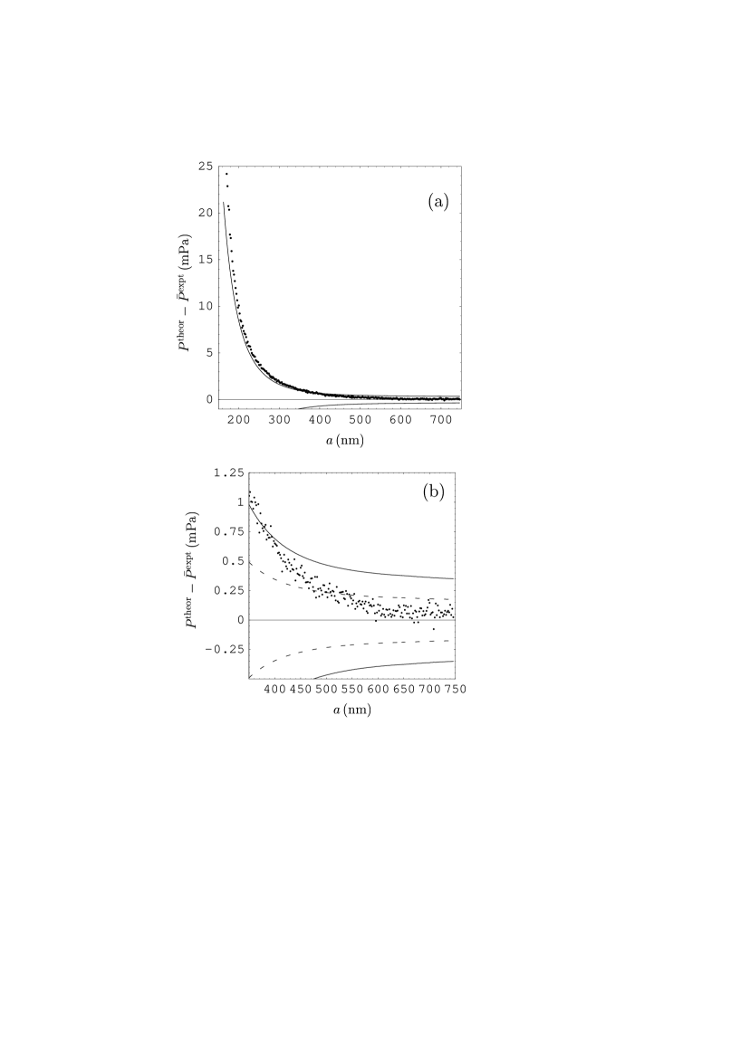
Figure 6: Differences between theoretical and mean experimental Casimir pressures are indicated as dots. Computations are performed using the Lifshitz formula at $T=0$ and the generalized plasma-like dielectric permittivity with the largest of other suggested plasma frequencies for separations (a) from 160 to 750 nm and (b) from 350 to 750 nm. Solid and dashed lines indicate the borders of 95% and 70% confidence intervals, respectively.

Now we compare the experimental data 21 ; 22 with the predictions from the Lifshitz formula at zero temperature combined with the generalized plasma-like model when other suggested values for the plasma frequency are used. We have performed computations of the Casimir pressure by using Eqs. (1), (2) and (11) with the largest suggested mean plasma frequency $\omega_{p}=8.38\,$eV found 35 (see Sec. III). The computational results for $P^{\rm theor}(a)-\bar{P}^{\rm expt}(a)$ are indicated as dots in Fig. 6 within the separation regions (a) from 160 to 750 nm and (b) from 350 to 750 nm. The solid lines indicate the borders of the 95% confidence intervals. For the comparison purposes, the dashed lines in Fig. 6(b) show the borders of the 70% confidence intervals. As can be seen in Fig. 6, the experimental data exclude the theoretical prediction from the zero-temperature Lifshitz formula with the value of $\omega_{p}^{(5)}$ at a 95% confidence level within the range of separations from 160 to 370 nm. From Fig. 6(b) it follows also that at a 70% confidence level the same theoretical predictions are excluded over a wider separation region from 160 to 480 nm. It must be emphasized that for all other suggested plasma frequencies from 6.82 to 8.38 eV considered 35 the magnitudes of computed theoretical Casimir pressures, $P^{\rm theor}(a)$, are less than for $\omega_{p}^{(5)}=8.38\,$eV. As a result, these theoretical predictions are experimentally excluded at a 95% confidence level over a wider separation region than in Fig. 6. The values of the plasma frequency from 8.38 eV to approximately 8.44 eV are also excluded at a 95% confidence level over a bit more narrow separation region than in Fig. 6. As to the values of the plasma frequency from 8.45 to 8.65 eV, they are excluded by the experimental data 21 ; 22 at a 70% confidence level over different regions of separations.

VI Conclusions and discussion

In the foregoing we have compared the experimental data of the experiment on an indirect dynamic measurement of the Casimir pressure between two parallel Au plates 21 ; 22 with the predictions of the zero-temperature Lifshitz theory computed employing the optical data extrapolated to zero frequency by the Drude model with both most often used or other suggested Drude parameters. We have also performed the comparison of the same data with the computational results obtained with the help of the zero-temperature Lifshitz formula combined with the generalized plasma-like dielectric permittivity with either most often used or other values of the plasma frequency.

The main conclusion obtained from these comparisons is that the zero-temperature Lifshitz theory combined with the Drude model is excluded by the experimental data for the Casimir pressure at short separations below $1\,\mu$m. In the case when the optical data are extrapolated to low frequencies by means of the Drude model with most often used parameters, the exclusion occurs at a 70% confidence level. If the extrapolation uses other suggested parameters of the Drude model, the zero-temperature Lifshitz theory is excluded by the data at a 95% confidence level. The theoretical predictions from the zero-temperature Lifshitz formula combined with the generalized plasma-like dielectric permittivity with the most often used value of the plasma frequency are shown to be experimentally consistent. The same theoretical approach but with other suggested values for the plasma frequency is excluded at a 95% confidence level. Keeping in mind that the experimental data for the Casimir force and Casimir pressure in previous experiments were obtained at room temperature $T=300\,$K and that the Lifshitz formula at zero temperature but with room-temperature Drude parameters has no clear physical meaning, conclusion is made that it is more consistent to compare all such kind of data with the Lifshitz theory at nonzero temperature.

The disagreement of the experimental data 21 ; 22 with theory involving the Drude model with other suggested parameters 35 ; 42 at both zero and nonzero temperature (for the latter case it was demonstrated in Refs. 2 ; 3 ; 52 ) raises several important questions. The dielectric response of conductors on real electromagnetic field of sufficiently low frequencies is described beyond any reasonable doubt by the Drude model. However, substitution of this model with both most often used and other suggested sets of Drude parameters in the Lifshitz formula for the Casimir force at any temperature (zero or nonzero) results in contradictions with the experimental data. This suggests that there might be some deep unclarified differences between fluctuating electromagnetic field considered in the Lifshitz theory and real electromagnetic field 27 . Measurements of the optical properties 35 with different Au films deposited on different substrates unequivocally demonstrated that these properties depend on the method of preparation of the film and can vary from sample to sample. Observed variations, however, are mostly determined by the relaxation properties of conduction electrons in thin films. The attempt to describe respective optical data by the simple Drude model with a frequency-independent relaxation parameter results in sample-to-sample variation of both Drude parameters. However, one should take proper account of the fact that the Casimir pressures computed with the help of the Drude model with any of the suggested Drude parameters are experimentally excluded by the experiments 20 ; 21 ; 22 while the theoretical results obtained employing the generalized plasma-like model with the most often used value of the plasma frequency are experimentally consistent. Then it is natural to suggest that the dielectric permittivity in the Lifshitz theory should not be considered in the standard way as obtained from a response of a metal film to a real electromagnetic field. It appears as if the dielectric permittivity in the Lifshitz theory directly accounts for the contribution of core electrons, but treats conduction electrons as a nondissipative plasma.

As it was mentioned in the Introduction, there are experiments of three different types with metallic 19 ; 20 ; 21 ; 22 ; 43 , semiconductor 23 ; 24 and dielectric 25 ; 26 test bodies which cast doubts on the use of the Drude model in the Lifshitz theory. Some complicated issues related to all experiments on measuring the Casimir force were discussed in Sec. II. Keeping in mind that experiments on measuring very small forces and separations are rather complicated, it would be of much interest to have additional independent confirmation of the obtained results. Such kind of experiments can be proposed. For this purpose one should use two micromachined oscillators with the same Au-coated spheres, as in Refs. 20 ; 21 ; 22 ; 43 , but with Au-coatings on the plates made as suggested in Ref. 35 . In one oscillator the plate should be coated with Au following the deposition procedure 35 used for the sample N1 ($\omega_{p}^{(1)}=6.82\,$eV and $\gamma^{(1)}=40.5\,$meV). For the second oscillator the Au coating on the plate should be performed 35 as for the sample N5 ($\omega_{p}^{(5)}=8.38\,$eV and $\gamma^{(5)}=37.1\,$meV). In fact it would be sufficient that the characteristic sizes of grains in Au-coatings on the two plates be markedly different 35 . In this case it is easily seen that the respective difference in the Casimir pressures computed for the two oscillators using the Drude model with such different parameters is several times larger than the total experimental error of pressure measurements within a wide region of separations. If the mean Casimir pressures measured with two oscillators would be different, it would demonstrate the role of relaxation of conduction electrons. If, however, in both cases the same Casimir pressures are obtained, it would confirm that relaxation properties of conduction electrons do not influence the Casimir effect and should be disregarded. To perform the suggested experiment, the measurement scheme of a difference-type can be used 53 ; 54 . In this case two halves of the plate of an oscillator are made using different deposition procedures (one-half is covered with Au-coating consisting of large grains and another-half of small grains). When such a patterned plate moves back and forth below the sphere, the measured difference Casimir force would be nonvanishing (vanishing) depending on the role of relaxation of free charge carriers. Thus, the result of this experiment can give the ultimate answer to the question whether the relaxation properties of conduction electrons influence the Casimir force.

Figure 1: Experimental data for the Casimir pressure (crosses) as a function of separation and the theoretical band between the two solid lines computed employing the Lifshitz formula at $T=0$ and the Drude extrapolation of the optical data with most often used parameters. The arms of the crosses and the widths of the bands are determined at (a) 95% confidence level and (b) 70% confidence level.

Figure 2: Differences between theoretical and mean experimental Casimir pressures are indicated as dots. Computations are performed employing the Lifshitz formula at $T=0$ and the Drude extrapolation of the optical data with most often used parameters. Solid and dashed lines indicate the borders of 95% and 70% confidence intervals, respectively.

Figure 3: Experimental data for the Casimir pressure (crosses) determined at a 95% confidence level and the theoretical band between the two solid lines computed employing the Lifshitz formula at $T=0$ and the Drude extrapolation of the optical data with different sets of parameters for separations (a) from 300 to 350 nm and (b) from 350 to 400 nm. The widths of the bands are determined at a 95% confidence level.

Figure 4: Differences between theoretical and mean experimental Casimir pressures are indicated as dots. Computations are performed using the Lifshitz formula at $T=0$ and the Drude extrapolation of the optical data with different sets of parameters (the upper and lower sets of dots correspond to smaller and larger plasma frequency, respectively) for separations (a) from 160 to 750 nm and (b) from 500 to 750 nm. Solid and dashed lines indicate the borders of 95% and 70% confidence intervals, respectively.

Figure 5: Differences between theoretical and mean experimental Casimir pressures are indicated as dots. Computations are performed employing the Lifshitz formula at $T=0$ and the generalized plasma-like dielectric permittivity with the most often used value of the plasma frequency. Solid and dashed lines indicate the borders of 95% and 70% confidence intervals, respectively.

References

- (1) H. B. G. Casimir, Proc. K. Ned. Akad. Wet. 51, 793 (1948).
- (2) M. Bordag, G. L. Klimchitskaya, U. Mohideen, and V. M. Mostepanenko, Advances in the Casimir Effect (Oxford University Press, Oxford, 2009).
- (3) G. L. Klimchitskaya, U. Mohideen, and V. M. Mostepanenko, Rev. Mod. Phys. 81, 1827 (2009).
- (4) E. M. Lifshitz, Zh. Eksp. Teor. Fiz. 29, 94 (1956) [Sov. Phys. JETP 2, 73 (1956)].
- (5) I. E. Dzyaloshinskii, E. M. Lifshitz, and L. P. Pitaevskii, Usp. Fiz. Nauk 73, 381 (1961) [Adv. Phys. 38, 165 (1961)].
- (6) E. M. Lifshitz and L. P. Pitaevskii, Statistical Physics, Part. II (Pergamon Press, Oxford, 1980).
- (7) T. Emig, R. L. Jaffe, M. Kardar, and A. Scardicchio, Phys. Rev. Lett. 96, 080403 (2006).
- (8) T. Emig, N. Graham, R. L. Jaffe, and M. Kardar, Phys. Rev. D 77, 025005 (2008).
- (9) O. Kenneth and I. Klich, Phys. Rev. Lett. 97, 160401 (2006).
- (10) O. Kenneth and I. Klich, Phys. Rev. B 78, 014103 (2008).
- (11) A. Bulgac, P. Magierski, and A. Wirzba, Phys. Rev. D 73, 025007 (2006).
- (12) M. Bordag, Phys. Rev. D 73, 125018 (2006).
- (13) A. Lambrecht and V. N. Marachevsky, Phys. Rev. Lett. 101, 160403 (2008).
- (14) H.-C. Chiu, G. L. Klimchitskaya, V. N. Marachevsky, V. M. Mostepanenko, and U. Mohideen, Phys. Rev. B 80, 121402(R) (2009).
- (15) H.-C. Chiu, G. L. Klimchitskaya, V. N. Marachevsky, V. M. Mostepanenko, and U. Mohideen, Phys. Rev. B 81, 115417 (2010).
- (16) M. Boström and B. E. Sernelius, Phys. Rev. Lett. 84, 4757 (2000).
- (17) I. Brevik, J. B. Aarseth, J. S. Høye, and K. A. Milton, Phys. Rev. E 71, 056101 (2005).
- (18) I. Brevik, S. A. Ellingsen, J. S. Høye, and K. A. Milton, J. Phys. A: Math. Theor. 41, 164017 (2008).
- (19) R. S. Decca, E. Fischbach, G. L. Klimchitskaya, D. E. Krause, D. López, and V. M. Mostepanenko, Phys. Rev. D 68, 116003 (2003).
- (20) R. S. Decca, D. López, E. Fischbach, G. L. Klimchitskaya, D. E. Krause, and V. M. Mostepanenko, Ann. Phys. (N.Y.) 318, 37 (2005).
- (21) R. S. Decca, D. López, E. Fischbach, G. L. Klimchitskaya, D. E. Krause, and V. M. Mostepanenko, Phys. Rev. D 75, 077101 (2007).
- (22) R. S. Decca, D. López, E. Fischbach, G. L. Klimchitskaya, D. E. Krause, and V. M. Mostepanenko, Eur. Phys. J. C 51, 963 (2007).
- (23) F. Chen, G. L. Klimchitskaya, V. M. Mostepanenko, and U. Mohideen, Optics Express 15, 4823 (2007).
- (24) F. Chen, G. L. Klimchitskaya, V. M. Mostepanenko, and U. Mohideen, Phys. Rev. B 76, 035338 (2007).
- (25) J. M. Obrecht, R. J. Wild, M. Antezza, L. P. Pitaevskii, S. Stringari, and E. A. Cornell, Phys. Rev. Lett. 98, 063201 (2007).
- (26) G. L. Klimchitskaya and V. M. Mostepanenko, J. Phys. A: Math. Theor. 41, 312002(F) (2008).
- (27) V. M. Mostepanenko and G. L. Klimchitskaya, ArXiv:0912.3877, Int. J. Mod. Phys, A 25 (2010), to appear.
- (28) G. Bressi, G. Carugno, R. Onofrio, and G. Ruoso, Phys. Rev. Lett. 88, 041804 (2002).
- (29) M. Lisanti, D. Iannuzzi, and F. Capasso, Proc. Natl. Acad. Sci. U.S.A. 102, 11989 (2005).
- (30) G. Jourdan, A. Lambrecht, F. Comin, and J. Chevrier, Europhys. Lett. 85, 31001 (2009).
- (31) P. J. van Zwol, G. Palasantzas, and J. Th. M. De Hosson, Phys. Rev. B 79, 195428 (2009).
- (32) V. B. Bezerra, G. L. Klimchitskaya, and V. M. Mostepanenko, Phys. Rev. A 66, 062112 (2002).
- (33) M. Antezza, L. P. Pitaevskii, S. Stringari, and V. B. Svetovoy, Phys. Rev. A 77, 022901 (2008).
- (34) Handbook of Optical Constants of Solids, ed. E. D. Palik (Academic, New York, 1985).
- (35) A. Lambrecht and S. Reynaud, Eur. Phys. J. D 8, 309 (2000).
- (36) V. B. Svetovoy, P. J. van Zwol, G. Palasantzas, and J. Th. M. De Hosson, Phys. Rev. B 77, 035439 (2008).
- (37) G. Bimonte, Phys. Rev. A 81, 062501 (2010).
- (38) G. L. Klimchitskaya, U. Mohideen, and V. M. Mostepanenko, J. Phys. A: Math. Theor. 40, F339 (2007).
- (39) J. Blocki, J. Randrup, W. J. Swiatecki, and C. F. Tsang, Ann. Phys. (N.Y.) 105, 427 (1977).
- (40) S. G. Rabinovich, Measurement Errors and Uncertainties. Theory and Practice (Springer-Verlag, New York, 2000).
- (41) G. L. Klimchitskaya, F. Chen, R. S. Decca, E. Fischbach, D. E. Krause, D. López, U. Mohideen, and V. M. Mostepanenko, J. Phys. A: Math. Gen. 39, 6485 (2006).
- (42) I. Pirozhenko, A. Lambrecht, and V. B. Svetovoy, New J. Phys. 8, 238 (2006).
- (43) R. S. Decca, D. López, and E. Osquiguil, Int. J. Mod. Phys. A 25 (2010), to appear.
- (44) W. J. Kim, M. Brown-Hayes, D. A. R. Dalvit, J. H. Brownell, and R. Onofrio, Phys. Rev. A 78, 020101(R) (2008).
- (45) R. S. Decca, E. Fischbach, G. L. Klimchitskaya, D. E. Krause, D. López, U. Mohideen, and V. M. Mostepanenko, Phys. Rev. A 79, 026101 (2009).
- (46) R. S. Decca and D. López, Int. J. Mod. Phys. A 24, 1748 (2009).
- (47) Q. Wei, D. A. R. Dalvit, F. C. Lombardo, F. D. Mazzitelli, and R. Onofrio, Phys. Rev. A 81, 052115 (2010).
- (48) S. de Man, K. Heeck, and D. Iannuzzi, Phys. Rev. A 79, 024102 (2009).
- (49) W. J. Kim, A. O. Sushkov, D. A. R. Dalvit, and S. K. Lamoreaux, Phys. Rev. A 81, 022505 (2010).
- (50) C. C. Speake and C. Trenkel, Phys. Rev. Lett. 90, 160403 (2003).
- (51) V. M. Mostepanenko, J. Phys.: Conf. Ser. 161, 012003 (2009).
- (52) R. S. Decca, D. López, H. B. Chan, E. Fischbach, D. E. Krause, and C. R. Jamell, Phys. Rev. Lett. 94, 240401 (2005).
- (53) R. Castillo-Garza, C.-C. Chang, D. Jimenez, G. L. Klimchitskaya, V. M. Mostepanenko, and U. Mohideen, Phys. Rev. A 75, 062114 (2007).