AC-driven vortices and the Hall effect in a tilted washboard planar pinning potential

Abstract

The Langevin equation for a two-dimensional (2D) nonlinear guided vortex motion in a tilted cosine pinning potential in the presence of an ac current is exactly solved in terms of a matrix continued fraction at arbitrary value of the Hall effect. The influence of an ac current of arbitrary amplitude and frequency on the dc and ac magnetoresistivity tensors is analyzed. The $ac$ current density and frequency dependence of the overall shape and the number and position of the Shapiro steps on the anisotropic current-voltage characteristics is considered. An influence of a subcritical or overcritical dc current on the time-dependent stationary ac longitudinal and transverse resistive vortex response (on the frequency of an ac-driving $\Omega$) in terms of the nonlinear impedance tensor $\hat{Z}$ and a nonlinear ac response at $\Omega$-harmonics are studied. New analytical formulas for $2D$ temperature-dependent linear impedance tensor $\hat{Z}_{L}$ in the presence of a dc current which depend on the angle $\alpha$ between the current density vector and the guiding direction of the washboard PPP are derived and analyzed. Influence of $\alpha$-anisotropy and the Hall effect on the nonlinear power absorption by vortices is discussed.

I Introduction

It is well known that the mixed-state resistive properties of type-II superconductors are determined by the dynamics of vortices which in the presence of pinning sites may be described as a motion of vortices in some pinning potential BLAT . In the simplest case this pinning potential is assumed to be periodic in one dimension, and temperature-dependent $dc$ current uniaxial pinning anisotropy, provoked by such washboard planar pinning potential (PPP) recently has been extensively studied both theoretically^2-4 and experimentally.^5-9 Two main reasons stimulated these studies. First, in some high-$T_{c}$ superconductors (HTSCs) twins can easily be formed during the crystal growth.^5-7 Second, in layered HTSCs the system of interlayers between parallel $ab$-planes can be considered as a set of unidirectional planar defects which provoke the intrinsic pinning of vortices. BLAT

As the pinning force in a PPP is directed perpendicular to the washboard channels of the PPP BLAT , the vortices generally tend to move along these channels. Such a guided motion of vortices in the presence of the Hall effect produces anisotropic transport behaviour for which even (+) and odd (–) (with respect to the magnetic field reversal) longitudinal ($\parallel$) and transverse ($\perp$) $dc$ nonlinear magnetoresistivities $\rho_{\parallel,\perp}^{dc\pm}$ depend substantially on the angle $\alpha$ between the $dc$ current density vector $\mathbf{j}$ and the direction of the PPP channels (”guiding direction”).

The $dc$-current nonlinear guiding problem was exactly solved recently for the washboard PPP within the framework of the two-dimensional ($2D$) single-vortex stochastic model of anisotropic pinning based on the Fokker-Planck equation and rather simple formulas were derived for the $dc$ magnetoresistivities $\rho_{\parallel,\perp}^{\pm}$.MAW ; SSS

On the other hand, the high-frequency and microwave impedance measurements of a mixed state can also give information about the flux pinning mechanisms and the vortex dynamics. One of the most popular experimental methods for the investigation of the vortex dynamics in type-II superconductors is the measurement of the complex $ac$ response in the radiofrequency and microwave ranges. When the Lorentz force acting on the vortices is alternating, then due to the pinning the $ac$ resistive response acquires imaginary (out-of-phase) component. Due to this reason measurements of the complex $ac$ response versus frequency $\omega$ can give important information on the pinning forces.

The very early model of Gittleman and Rosenblum GR (GR) considered oscillations of damped vortex in a garmonic pinning potential. GR measured the power absorption of the vortices in PbIn and NbTa films over a wide range of frequencies $\omega$ and successfully analyzed their data with the simple equation

$$\eta\dot{x}+k_{p}x=F_{L},$$ (1)

where $x$ is the vortex displacement, $\eta$ is the vortex viscosity, $k_{p}$ is the pinning constant, and $F_{L}$ is the Lorentz force. From Eq. (1) follows that the complex vortex resistivity $\rho_{v}$ is

$$(\rho_{v}/\rho_{f})=i(\omega/\omega_{p})/[1+i(\omega/\omega_{p})],$$ (2)

where $\rho_{f}$ is the flux-flow resistivity and $\omega_{p}\equiv k_{p}/\eta$ is the depinning frequency. As follows from Eqs. (1) and (2), pinning forces dominate at low frequencies ($\omega\ll\omega_{p}$) where $\rho_{v}$ is nondissipative, whereas at high frequencies ($\omega\gg\omega_{p}$) frictional forces dominate and the vortex resistivity is dissipative.

The experimental success of this very simple model stimulated the attempts to use it for the interpretation of the data taken in HTCSs, where the effects of thermal agitation are especially important due to their low pinning activation energies and the high temperatures of the superconducting state. As the GR model was developed for zero temperature and could not account for the thermally activated flux flow and creep, which are very pronounced in HTCSs, there was a need for a more general model for the $ac$ vortex dissipation at different temperatures and frequencies.

In order to fulfill this aim the vortex equation of motion (1) was supplemented with Langevin force which was assumed to be Gaussian white noise with zero mean and the cosine periodic pinning potential was used^11-13 for taking into account the possibility of vortex hopping between different potential wells. In the limit of small $ac$ current (i. e. for a nontilted cosine pinning potential) this new equation of motion was approximately solved by a continued-fraction expansion^11-13 using the analogy between a pinned vortex and a Brownian particle motion in a periodic potential. As a result, the complex resistivity $\rho_{v}$ which generalizes the GR‘s Eq. (2) has the form (see Eq. (8) in Ref. 11)

$$\quad(\rho_{v}/\rho_{f})=[i(\omega/\omega_{0})+\nu_{00}]/[1+i(\omega/\omega_{0})],$$ (3)

where $\nu_{00}$ is a creep factor that grows monotonically with temperature increasing from $\nu_{00}=0$ (no flux creep) to $\nu_{00}=1$ (flux flow regime) and $\omega_{0}$ is a characteristic frequency (nonmonotonic in temperature) which, in absence of creep, corresponds to the depinning frequency $\omega_{p}$. If the frequency $\omega$ is swept across the temperature-dependent frequency $\omega_{0}$, the observed $\textrm{Re}\rho_{v}$ increases from a low frequency value to the flux-flow value $\rho_{f}$ while $\textrm{Im}\rho_{v}$ exhibits a maximum at $\omega_{0}$. Thus, we can summarize that the temperature-dependent $ac$-driven vortex motion problem has been exactly solved so far only for the one-dimensional (1D) nontilted cosine pinning potential at a small oscillation amplitude of the vortices.

At the same time, the examination of a strong $ac$-driving (that is interesting both for theory and for different high-frequency or microwave applications) evidently requires to consider strongly tilted pinning potential. Actually, if at low temperatures and relatively high frequencies in nontilted pinning potential each pinned vortex will be confined to its pinning potential well during the $ac$ period, in the case of strong $ac+dc$ driving current the running states of the vortex may appear when it can visit several (or many) potential wells during the $ac$ period.

The aim of this work is to suggest a new theoretical approach to the study of temperature-dependent nonlinear ac-driven pinning-mediated vortex dynamics based on an exact solution (in terms of a matrix continued fraction) of the same equation of vortex motion, as was discussed by Coffey and Clem (CC) in the seminal paper CLEM (see below Eq. (4) which has an additional Hall term). This new approach substantially generalizes the CC‘s results because the two-dimensional (2D) Langevin equation for the nonlinear guided motion in a tilted cosine PPP in the presence of a strong $ac$ current at arbitrary value of the Hall effect has been exactly solved. For this exact solution we used the matrix continued fraction technique earlier suggested and later extensively employed for calculation of $1D$ nonlinear ($ac+dc$)-driven response of overdamped Josephson junction with noise in Refs. 14, 15.

As a result, two groups of new findings were obtained. First, for previously solved in Refs. 2 and 3 the $2D$ $dc$-problem of the influence of an $ac$ current on the overall shape and appearance of the Shapiro steps on the anisotropic $dc$ $\rho_{\parallel,\perp}^{dc\pm}$ – CVC‘s was calculated and analyzed. Second, for the $ac$ current at a frequency $\omega$ plus $dc$ bias the $2D$ nonlinear time-dependent stationary $\rho_{\parallel,\perp}^{ac\pm}$ $ac$-response on the frequency $\omega$ in terms of nonlinear impedance tensor $\hat{Z}$ and a nonlinear ac response at $\omega$-harmonics was studied.

The organization of the paper is as follows. In Sec. II we introduce the model and the basic quantities of interest, namely, the average two-dimensional electric field and the Fourier amplitudes for the averaged moments $\langle r^{m}\rangle$. In Sec. III we present the solution of the recurrence equations for the Fourier amplitudes in terms of matrix continued fraction and introduce the main anisotropic nonlinear component of our theory – the average pinning force, divided into three parts. In Sec. IV we discuss the $\omega$-dependent $dc$ current magnetoresistivity response with different (from A to E subsections) aspects of this problem. Section V (with subsections from A to H ) represents different problems related to nonlinear anisotropic stationary ac response. In Sec. VI we conclude with a general discussion of our results.

II Formulation of the problem

The Langevin equation for a vortex moving with velocity $\mathbf{v}$ in a magnetic field $\mathbf{B}=\mathbf{n}B$ ($B\equiv|\mathbf{B}|$, $\mathbf{n}=n\mathbf{z}$, $\mathbf{z}$ is the unit vector in the $z$ direction and $n=\pm 1$) has the form

$$\eta\mathbf{v}+n\alpha_{H}\mathbf{v}\times\mathbf{z}=\mathbf{F}_{L}+\mathbf{F}_{p}+\mathbf{F}_{th},$$ (4)

where $\mathbf{F}_{L}=n(\Phi_{0}/c)\mathbf{j}\times\mathbf{z}$ is the Lorentz force ($\Phi_{0}$ is the magnetic flux quantum, and $c$ is the speed of light), $\mathbf{j}=\mathbf{j}(t)=\mathbf{j}^{dc}+\mathbf{j}^{ac}\cos\omega t$, where $\mathbf{j}^{dc}$ and $\mathbf{j}^{ac}$ are the $dc$ and $ac$ current density amplitudes and $\omega$ is the angular frequency, $\mathbf{F}_{p}=-\nabla U_{p}(x)$ is the anisotropic pinning force ($U_{p}(x)$ is the washboard planar pinning potential), $\mathbf{F}_{th}$ is the thermal fluctuation force, $\eta$ is the vortex viscosity, and $\alpha_{H}$ is the Hall constant. We assume that the fluctuational force $\mathbf{F}_{th}(t)$ is represented by a Gaussian white noise, whose stochastic properties are assigned by the relations

$$\langle F_{th,i}(t)\rangle=0,\,\langle F_{th,i}(t)F_{th,j}(t^{\prime})\rangle=2T\eta\delta_{ij}\delta(t-t^{\prime}),$$ (5)

where $T$ is the temperature in energy units, $\langle...\rangle$ means the statistical average, and $F_{th,i}(t)$ with $i=x$ or $i=y$ is the $i$ component of $\mathbf{F}_{th}(t)$.

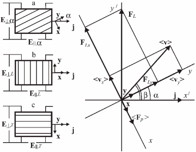
Figure 1: System of coordinates $xy$ (with the unit vectors $\mathbf{x}$ and $\mathbf{y}$) associated with the PPP washboard channels and the system of coordinates $x^{\prime}y^{\prime}$ associated with the direction of the current density vector $\mathbf{j}$; $\alpha$ is the angle between the channels of the PPP and $\mathbf{j}$, $\beta$ is the angle between the average velocity vector of the vortices $\langle\textbf{v}\rangle$ and $\mathbf{j}$; $\mathbf{F}_{L}$ is the Lorentz force; $<\mathbf{F}_{p}>$ is the average pinning force, $\mathbf{F}_{Lx}$ is the average effective motive force for a vortex. Here for simplicity we assume $\epsilon=0$. The schematic sample configuration for three cases with different values of angle $\alpha$ (the insert): general case, $\alpha\neq 0,\pi/2$ (a); longitudinal $L$-geometry, $\alpha=\pi/2$, $\mathbf{j}\perp\mathbf{y}$ (b); transverse $T$-geometry, $\alpha=0$, $\mathbf{j}\perp\mathbf{x}$ (c); in all cases $E_{\perp}$ and $E_{\parallel}$ are transverse and longitudinal (with respect to $\mathbf{j}$-direction) electric field components.

The formal statistical average of Eq. (4) is

$$\eta\langle\mathbf{v}\rangle+n\alpha_{H}\langle\mathbf{v}\rangle\times\mathbf{z}=\mathbf{F}_{L}+\langle\mathbf{F}_{p}\rangle.$$ (6)

Though $\langle\mathbf{F}_{th}\rangle$ disappears because of the stochastic property in Eq. (5), effects of the thermal fluctuation are implicit in the term $\langle\mathbf{F}_{p}\rangle$ (see below).

Since the anisotropic pinning potential is assumed to depend only on the $x$ coordinate and is assumed to be periodic ($U_{p}(x)=U_{p}(x+a)$, where $a$ is the period), the pinning force is always directed along the anisotropy axis $x$ (with unity vector x, see Fig. 1) so that it has no component along the $y$ axis ($F_{py}=-dU_{p}/dy=0$). Thus, Eq. (4) reduces to the equations

$$\left\{\begin{array}[]{lll}v_{x}+\delta v_{y}=(F_{Lx}+F_{px}+F_{x}/)\eta,\\ \\ v_{y}-\delta v_{x}=(F_{Ly}+F_{y})/\eta,\\ \end{array}\right.$$ (7)

where $\delta\equiv n\epsilon$, $\epsilon\equiv\alpha_{H}/\eta$, and we omitted index $th$ in the $\mathbf{F}_{th}$ for simplicity. Eqs. (7) can be rewritten for the subsequent analysis in the following form

$$\begin{array}[]{crr}v_{x}\equiv\dot{x}=(\tilde{F}_{Lx}+F_{px}+\tilde{F}_{x})/\eta D,\\ \\ v_{y}\equiv\dot{y}=(\tilde{F}_{Ly}+\tilde{F}_{y}+\delta F_{px})/\eta D.\\ \end{array}$$ (8)

where $\tilde{F}_{Lx}\equiv F_{Lx}-\delta F_{Ly}$, $\tilde{F}_{Ly}\equiv F_{Ly}+\delta F_{Lx}$, $\tilde{F}_{x}\equiv F_{x}-\delta F_{y}$, $\tilde{F}_{y}\equiv F_{y}+\delta F_{x}$, $D\equiv 1+\delta^{2}$ and $\langle\tilde{F}_{i}(t)\tilde{F}_{j}(t^{\prime})\rangle=2T\eta D\delta_{ij}\delta(t-t^{\prime})$.

Our aim now is to obtain from Eqs. (8) a rigorous and explicit expression of $\langle v_{x}\rangle$ and $\langle v_{y}\rangle$ in which effects of the pinning and the thermal fluctuation are considered. We assume, as usual^2,11-13, a periodic pinning potential of the form $U_{p}(x)=(U_{p}/2)(1-\cos kx))$ where $k=2\pi/a$. As $F_{px}=-F_{p}\sin kx$, where $F_{p}\equiv U_{p}k/2$, the first from Eqs. (8) has the form

$$\hat{\tau}(d\textsl{x}/dt)+\sin\textsl{x}=\hat{F}_{Lx}+\hat{F}_{x}.$$ (9)

Here $\textsl{x}=kx$ is the dimensionless vortex coordinate, $\hat{\tau}\equiv\eta D/kF_{p}$ is the relaxation time, $\hat{F}_{Lx}=\tilde{F}_{Lx}/F_{p}$ is the dimensionless generalized moving force in the $x$ direction, $\hat{F}_{x}=\tilde{F}_{x}/F_{p}$, and $\langle\hat{F}_{x}(t)\hat{F}_{x}(t^{\prime})\rangle=\tau\delta(t-t^{\prime})$, where $\tau\equiv\hat{2\tau}/g$ and $g=U_{p}/2T$ is the dimensionless inverse temperature.

Making the transformation $\textsl{x}(t)\rightarrow r^{m}(t)=e^{-im\textsl{x}(t)}$ in Eq. (9) one obtains a stochastic differential equation with a multiplicative noise term, the averaging of which yields a system of differential-recurrence relations for the moments $\langle r^{m}\rangle=\langle e^{-im\textsl{x}}\rangle$ (as described in detail in Ref. [14]), viz.,

$$\begin{array}[]{ll}\hat{\tau}d\langle r^{m}\rangle(t)/dt+[m^{2}/g+im\hat{F}_{Lx}]\langle r^{m}\rangle(t)=\\ \\ \qquad{}=(m/2)(\langle r^{m-1}\rangle(t)-\langle r^{m+1}\rangle(t)).\\ \end{array}$$ (10)

The main quantity of physical interest in our problem is the average electric field, induced by the moving vortex system, which is given by

$$\langle\mathbf{E}\rangle=(n/c)\mathbf{B}\times\langle\mathbf{v}\rangle=n(B/c)(-\langle v_{y}\rangle\mathbf{x}+\langle v_{x}\rangle\mathbf{y}),$$ (11)

where $\mathbf{x}$ and $\mathbf{y}$ are the unit vectors in the $x$ and $y$ directions, respectively.

As follows from Eq. (8)

$$\langle v_{y}\rangle=F_{Ly}/\eta+\delta\langle v_{x}\rangle$$ (12)

and so for determination of $\langle\mathbf{E}\rangle$ from Eq. (11) it is sufficient to calculate the $\langle v_{x}\rangle$ from Eq. (9). This calculation gives

$$\langle v_{x}\rangle(t)=\frac{\Phi_{0}j_{c}}{c\eta D}[j^{dc}+j^{ac}\cos\omega t-\langle\sin\textsl{x}\rangle(t)],$$ (13)

where

$$\langle\sin\textsl{x}\rangle(t)=\frac{i}{2}[\langle r\rangle(t)-\langle r^{-1}\rangle(t)].$$ (14)

In Eq. (10) $j^{dc}\equiv n(j^{dc}_{y}+\delta j^{dc}_{x})/j_{c}$, $j^{ac}\equiv n(j^{ac}_{y}+\delta j^{ac}_{x})/j_{c}$, and $j_{c}\equiv cF_{p}/\Phi_{0}$.

Since we are only concerned with the stationary $ac$ response, which is independent of the initial condition, one needs to calculate the solution of Eq. (10) corresponding to the stationary case. To accomplish this, one may seek all the $\langle r^{m}\rangle(t)$ in the form

$$\langle r^{m}\rangle(t)=\sum_{\begin{subarray}{c}k=-\infty\end{subarray}}^{\begin{subarray}{c}\infty\end{subarray}}F_{k}^{m}(\omega)e^{ik\omega t}.$$ (15)

On substituting Eq. (15) into Eq. (10) we obtain recurrence equations for the Fourier amplitudes $F_{k}^{m}(\omega)$, i. e.,

$$\begin{array}[]{ll}F_{k}^{m+1}(\omega)-F_{k}^{m-1}(\omega)+iz_{m,k}(\omega)F_{k}^{m}(\omega)+\\ \\ \qquad{}+ij^{ac}[F_{k-1}^{m}(\omega)+F_{k+1}^{m}(\omega)]=0,\\ \end{array}$$ (16)

where

$$z_{m,k}(\omega)=2(j^{dc}+\omega\hat{\tau}k/m-im/g).$$ (17)

III The solution of the problem in terms of matrix continued fractions

The scalar five-term recurrence Eq. (16) can be transformed into the two uncoupled matrix three-term recurrence relations

$$\mathbf{Q}_{m}(\omega)\mathbf{C}_{m}(\omega)+\mathbf{C}_{m+1}(\omega)=\mathbf{C}_{m-1}(\omega),\quad(m=1,2,...)$$ (18)

and

$$-\mathbf{Q}_{m}^{\ast}(-\omega)\mathbf{C}_{-m}(\omega)+\mathbf{C}_{-m+1}(\omega)=\mathbf{C}_{-m-1}(\omega),\quad(m=1,2,...)$$ (19)

where $\mathbf{Q}_{m}$ is a tridiagonal infinite matrix given by

$$\mathbf{Q}_{m}(\omega)=i\begin{pmatrix}\ddots&\vdots&\vdots&\vdots&\ddots\\ \cdots&z_{m,-2}(\omega)&j^{ac}&0&\cdots\\ \cdots&j^{ac}&z_{m,-1}(\omega)&j^{ac}&0\\ \cdots&0&j^{ac}&z_{m,0}(\omega)&j^{ac}\\ \cdots&\cdots&0&j^{ac}&z_{m,1}(\omega)\\ \cdots&\cdots&\cdots&0&j^{ac}\\ \ddots&\vdots&\vdots&\vdots&\ddots\end{pmatrix},$$ (20)

(the asterisk denotes the complex conjugate) and the infinite column vectors $\mathbf{C}_{m}(\omega)$ are defined as

$$\begin{array}[]{ll}\mathbf{C}_{m}(\omega)=\begin{pmatrix}\vdots\\ F^{m}_{-2}(\omega)\\ F^{m}_{-1}(\omega)\\ F^{m}_{0}(\omega)\\ F^{m}_{1}(\omega)\\ F^{m}_{2}(\omega)\\ \vdots\end{pmatrix},\quad\textrm{for}\quad m=\pm 1,\pm 2,...\\ \textrm{and}\quad\mathbf{C}_{0}=\begin{pmatrix}\vdots\\ 0\\ 0\\ 1\\ 0\\ 0\\ \vdots\end{pmatrix},\quad\textrm{for}\quad m=0.\end{array}$$ (21)

Thus, in order to calculate $\langle\sin\textsl{x}\rangle(t)$ in Eq. (14), we need to evaluate $\mathbf{C}_{1}(\omega)$ and $\mathbf{C}_{-1}(\omega)$, which contain all the Fourier amplitudes of $\langle r\rangle(t)$ and $\langle r^{-1}\rangle(t)$. Equation (18) can be solved for $\mathbf{C}_{1}$ in terms of matrix continued fractions¹⁴, viz.,

$$\mathbf{C}_{1}(\omega)=\cfrac{\mathbf{I}}{\mathbf{Q}_{1}(\omega)+\cfrac{\mathbf{I}}{\mathbf{Q}_{2}(\omega)+\cfrac{\mathbf{I}}{\mathbf{Q}_{3}(\omega)+...}}}\mathbf{C}_{0},$$ (22)

where the fraction lines designate the matrix inversions and $\mathbf{I}$ is the identity matrix of infinite dimension. Having determined $\mathbf{C}_{1}(\omega)$, it is not necessary to solve Eq. (19), as all the components of the column vector $\mathbf{C}_{-1}(\omega)$ can be obtained from Eq. (22), on noting that

$$F_{0}^{1}(\omega)=F_{0}^{-1\ast}(\omega)\quad\textrm{and}\quad F_{k}^{-1}(\omega)=F_{-k}^{1\ast}(\omega).$$ (23)

Following the solutions of Eq. (22) and using relations (23), we can find the dimensionless average pinning force $\langle F_{px}\rangle(t)$ (see Eqs. (6)-(9), (14) and (15)) which is the main anisotropic nonlinear (due to a dependence on the $ac$ and $dc$ current input) component of the theory under discussion

$$\langle\hat{F}_{px}\rangle(t)=-\langle\sin\textsl{x}\rangle(t)=\sum_{\begin{subarray}{c}k=0\end{subarray}}^{\begin{subarray}{c}\infty\end{subarray}}\textrm{Im}(\psi_{k}e^{ik\omega t}),$$ (24)

where $\psi_{0}\equiv F_{0}^{1}(\omega)$ and for $k\geq 1$ we have $\psi_{k}\equiv F_{k}^{1}(\omega)-F_{k}^{-1}(\omega)$.

In fact, Eq. (24) is the expansion of the stationary time-dependent (and independent of the initial conditions) average pinning force $\langle\hat{F}_{px}\rangle(t)$ into three parts

$$\langle\hat{F}_{px}\rangle(t)=\langle\hat{F}_{px}\rangle_{0}^{\omega}+\langle\hat{F}_{px}\rangle_{t1}+\langle\hat{F}_{px}\rangle_{t}^{k>1}.$$ (25)

In Eq. (25) $\langle\hat{F}_{px}\rangle_{0}^{\omega}\equiv-\langle\sin\textsl{x}\rangle_{0}^{\omega}=\textrm{Im}\psi_{0}$ is the time independent (but frequency dependent) static average pinning force, which will be used for the derivation of the $dc$ magnetoresistivity tensor $\hat{\rho}_{0}^{\omega}$; $\langle\hat{F}_{px}\rangle_{t1}\equiv-\langle\sin\textsl{x}\rangle_{t1}=\textrm{Im}(\psi_{1}e^{i\omega t})$ is the time-dependent dynamic average pinning force with a frequency $\omega$ of the $ac$ current input, which is responsible for the nonlinear impedance $Z_{1}(\omega)$; $\langle\hat{F}_{px}\rangle_{t}^{k>1}\equiv-\langle\sin\textsl{x}\rangle_{t}^{k>1}=\textrm{Im}(\psi_{k}e^{ik\omega t})$ describes a contribution of the harmonics with $k>1$ into the dynamic average pinning force.

IV $\omega$-dependent dc current magnetoresistivity response

IV.1 The nonlinear DC resistivity and conductivity tensors

In order to proceed with these calculations we first express (see Eq. (11)) the time independent part of $\langle E_{y}\rangle(t)=(nB/c)\langle v_{x}\rangle(t)$ as

$$\begin{array}[]{ll}\langle E_{y}\rangle_{0}^{\omega}=(nB/c)\langle v_{x}\rangle_{0}^{\omega}\equiv(n\rho_{f}/D)(j^{dc}-\langle\sin\textsl{x}\rangle_{0}^{\omega})=\\ \\ \qquad\qquad\qquad=(\rho_{f}/D)\nu_{0}^{\omega}(j^{dc}_{y}+\delta j^{dc}_{x}),\end{array}$$ (26)

where

$$\nu_{0}^{\omega}\equiv 1-\langle\sin\textsl{x}\rangle_{0}^{\omega}/j^{dc}=1+\langle\hat{F}_{px}\rangle_{0}^{\omega}/j_{dc}.$$ (27)

In Eq. (26) $\rho_{f}\equiv B\Phi_{0}/\eta c^{2}$ is the flux-flow resistivity and the $\nu_{0}^{\omega}$ can be considered as the $(\omega,j^{dc},j^{ac},T)$-dependent effective mobility of the vortex under the influence of the dimensionless generalized moving force $\hat{F}_{Lx}^{dc}=j^{dc}$ in the $x$ direction. In the absence of the $ac$ current (see below Eq.(35)) the $\nu_{0}^{\omega}$ coincides with the probability of vortex hopping over the pinning potential barrier³.

From Eq. (27) follows another physical interpretation of the $\nu_{0}^{\omega}$ function, which has a close relationship to the average pinning force $\langle\hat{F}_{px}\rangle_{0}^{\omega}$ acting on the vortex. Actually, it is evident from Eq. (27) that the $\langle\hat{F}_{px}\rangle_{0}^{\omega}$ is connected to the $\nu_{0}^{\omega}$ function in a simple way,

$$\langle\hat{F}_{px}\rangle_{0}^{\omega}=-\hat{F}_{Lx}^{dc}(1-\nu_{0}^{\omega}).$$ (28)

Then it is easy to show that

$$\langle E_{x}\rangle_{0}^{\omega}=(\rho_{f}/D)[j^{dc}_{x}(1+\delta^{2}(1-\nu_{0}^{\omega}))-\delta j^{dc}_{y}].$$ (29)

From Eqs. (26) and (29) we find the $(\omega,j^{dc},j^{ac},T)$-dependent magnetoresistivity tensor for the $dc$-measured nonlinear law $\langle\mathbf{E}_{0}^{\omega}(\omega)\rangle=\hat{\rho}_{0}^{\omega}\mathbf{j}^{dc}$ as

$$\hat{\rho}_{0}^{\omega}=\begin{pmatrix}\rho_{xx}^{dc}&\rho_{xy}^{dc}\\ \rho_{yx}^{dc}&\rho_{yy}^{dc}\end{pmatrix}=\frac{\rho_{f}}{D}\begin{pmatrix}1+\delta^{2}(1-\nu_{0}^{\omega})&-\delta\nu_{0}^{\omega}\\ \delta\nu_{0}^{\omega}&\nu_{0}^{\omega}\end{pmatrix}.$$ (30)

The $dc$ conductivity tensor $\hat{\sigma}_{0}^{\omega}$, which is the inverse tensor to $\hat{\rho}_{0}^{\omega}$, has the form

$$\hat{\sigma}_{0}^{\omega}=\begin{pmatrix}\sigma_{xx}^{dc}&\sigma_{xy}^{dc}\\ \sigma_{yx}^{dc}&\sigma_{yy}^{dc}\end{pmatrix}=\frac{1}{\rho_{f}}\begin{pmatrix}1&\delta\\ -\delta&(D/\nu_{0}^{\omega})-\delta^{2}\end{pmatrix}.$$ (31)

We see from Eqs. (30) and (31) that the off-diagonal components of the $\hat{\rho}_{0}^{\omega}$ and $\hat{\sigma}_{0}^{\omega}$ tensors satisfy the Onsager relation ($\rho_{xy}=-\rho_{yx}$ in the general nonlinear case and $\sigma_{xy}=-\sigma_{yx}$). All the components of the $\hat{\rho}_{0}^{\omega}$ tensor and one of the diagonal components of the $\hat{\sigma}_{0}^{\omega}$ tensor are function of the current density $j^{dc}$, $j^{ac}$, and $\omega$ through the external force $\hat{F}_{Lx}$, the temperature $T$, the angle $\alpha$, and the dimensionless Hall parameter $\delta=n\epsilon$. It is important, however, to stress that the off-diagonal components of the $\hat{\sigma}_{0}^{\omega}$ are not influenced by a presence of the pinning potential barriers.

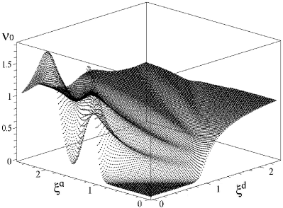
Figure 2: The dimensionless function $\nu_{0}^{\omega}(\xi^{d},\xi^{a})$ numerically obtained from Eq. (27) at $g=30$ and $\Omega=0.2$.

In conclusion of this subsection let us consider the limiting case $j^{ac}=0$, i. e. we should derive a static current-voltage characteristic (CVC). In this case we have from Eq. (10) that

$$(m+igj^{dc})\langle r^{m}\rangle_{0}=(g/2)(\langle r^{m-1}\rangle_{0}-\langle r^{m+1}\rangle_{0}),$$ (32)

where the subscript $"0"$ denotes the statistical average in the absence of the ac current. In order to solve Eq. (32) we introduce, following the calculation of RiskenRISK , the quantity $S_{m}=\langle r^{m}\rangle_{0}/\langle r^{m-1}\rangle_{0}$ which satisfies next equation

$$(m+igj^{dc})S_{m}=(g/2)(1-S_{m}S_{m+1}).$$ (33)

The solution of Eq. (33) (see details in Ref. [14]) can be expressed in terms of the modified Bessel functions $I_{\nu}(z)$ of the first kind of order $\nu$ (where $\nu$ may be a complex number Watson ) as

$$S_{m}=I_{m+\mu}(g)/I_{m-\mu}(g),$$ (34)

where $\mu\equiv igj^{dc}$. Taking into account Eqs. (27), (34), and the relation $S_{1}=\langle r\rangle_{0}=\langle\cos\textsl{x}\rangle_{0}-i\langle\sin\textsl{x}\rangle_{0}$ we conclude that $\langle\hat{F}_{px}\rangle_{0}=\textrm{Im}S_{1}=\textrm{Im}[I_{1+\mu}(g)/I_{\mu}(g)]$ and

$$\begin{array}[]{ccr}\nu_{0}\equiv\nu_{0}^{\omega}(j^{ac}=0,\omega=0)=1+\textrm{Im}S_{1}/j^{dc}=\\ \\ =1+\textrm{Im}[I_{1+\mu}(g)/I_{\mu}(g)]/j^{dc}.\\ \end{array}$$ (35)

Note that Eq. (35) gives a more simple analytical expression for the $\nu_{0}$ function which was presented in Ref. [2] on the basis of a Fokker-Planck approach, namely

$$\nu^{-1}_{0}(F)=\frac{F}{1-e^{-F}}\int_{\begin{subarray}{c}0\end{subarray}}^{\begin{subarray}{c}1\end{subarray}}due^{-Fu}I_{0}(2g\sin\pi u)$$ (36)

with $F\equiv 2\pi gj^{dc}$, where $g=U_{p}/2T$ is the dimensionless inverse temperature. In Fig. 2 we plotted $\nu_{0}^{\omega}(\xi^{d},\xi^{a})$ graphs at g=30 which demonstrate in the limit of $\xi^{a}=0$ the $\xi^{d}$-dependence for probability of vortex hopping over the tilted cosine pinning potential barrier; here $\xi^{d}$ and $\xi^{a}$ are the dimensionless $dc$ and maximal $ac$ current density magnitudes (in $j_{c}$ units), respectively ($\xi^{d}\equiv j^{d}/j_{c},\xi^{a}\equiv j^{a}/j_{c}$).

IV.2 Longitudinal and transverse DC resistivities

The experimentally measurable resistive $dc$ responses refer to coordinate system tied to the $dc$ current (see Fig. 1). The longitudinal and transverse (with respect to the $dc$ current direction) components of the electric field $E_{\parallel}^{dc}$ and $E_{\perp}^{dc}$, are related to $E_{x}^{dc}\equiv\langle E_{x}\rangle_{0}^{\omega}$ and $E_{y}^{dc}\equiv\langle E_{y}\rangle_{0}^{\omega}$ by the simple expressions

$$\begin{array}[]{crr}E_{\parallel}^{dc}=E_{x}^{dc}\sin\alpha+E_{y}^{dc}\cos\alpha,\\ \\ E_{\perp}^{dc}=-E_{x}^{dc}\cos\alpha+E_{y}^{dc}\sin\alpha.\\ \end{array}$$ (37)

Then according to Eqs. (37), the expressions for the experimentally observable longitudinal and transverse (with respect to the $\mathbf{j}^{dc}$ direction) magnetoresistivities $\rho_{\parallel}^{dc}=E_{\parallel}^{dc}/j^{d}$ and $\rho_{\perp}^{dc}=E_{\perp}^{dc}/j^{d}$ (where $j^{d}$ is the $dc$ current density $(j^{d})^{2}=(j_{x}^{dc})^{2}+(j_{y}^{dc})^{2}$) have the form

$$\begin{array}[]{crr}\rho_{\parallel}^{dc}=\rho_{xx}^{dc}\sin^{2}\alpha+\rho_{yy}^{dc}\cos^{2}\alpha,\\ \\ \rho_{\perp}^{dc}=\rho_{yx}^{dc}\sin^{2}\alpha-\rho_{xy}^{dc}\cos^{2}\alpha+(\rho_{yy}^{dc}-\rho_{xx}^{dc})\sin\alpha\cos\alpha.\\ \end{array}$$ (38)

Note, however, that the magnitudes of the $\rho_{\parallel}^{dc}$ and $\rho_{\perp}^{dc}$, given by Eqs. (38) and applied to the $dc$ current responses, in general, depend on the direction of the external magnetic field $\mathbf{B}$ along $z$ axis due to the $\delta=n\epsilon$ dependence of the $\nu_{0}^{\omega}$ function (see Eq. (27)). In order to consider only $n$-independent magnitudes of the $\rho_{\parallel}^{dc}$ and $\rho_{\perp}^{dc}$ responses we should introduce the even $(+)$ and odd $(-)$ magnetoresistivities with respect to magnetic field reversal ($\rho^{dc\pm}(n)\equiv[\rho^{dc}(n)\pm\rho^{dc}(-n)]/2$) for longitudinal and transverse dimensional magnetoresistivities, which in view of Eqs. (38) have the form

$$\begin{array}[]{ccr}\rho_{\parallel}^{dc\pm}=(\rho_{f}/D)[(\cos^{2}\alpha-\delta^{2}\sin^{2}\alpha)\nu_{0}^{\omega\pm}+\\ \\ +D(1\pm 1)\sin^{2}\alpha/2],\\ \end{array}$$ (39)

$$\begin{array}[]{ccr}\rho_{\perp}^{dc\pm}=(\rho_{f}/D)[D\nu_{0}^{\omega\pm}\sin\alpha\cos\alpha+\delta\nu_{0}^{\omega\mp}-\\ \\ -D(1\pm 1)\sin\alpha\cos\alpha/2],\\ \end{array}$$ (40)

where $\nu_{0}^{\omega\pm}(n)=[\nu_{0}^{\omega}(n)\pm\nu_{0}^{\omega}(-n)]/2$ are the even and odd components relative to the magnetic field inversion of the function $\nu_{0}^{\omega}(n)$. In the $E_{\parallel,\perp}^{dc+}(j)$ dependences, which follow from Eqs. (39) and (40), the nonlinear and linear (nonzero only for $\rho_{\parallel}^{dc+}$ and $\rho_{\perp}^{dc+}$) terms separate out in a natural way. The physical reason for the appearance of linear terms is that in the model under consideration for $\alpha\neq 0$ there is always the flux-flow regime of vortex motion along the channels of the PPP.

It follows from Eqs. (39) and (40) that for $\alpha\neq 0,\pi/2$ the observed resistive response contains not only the ordinary longitudinal $\rho_{\parallel}^{dc+}(\alpha)$ and transverse $\rho_{\perp}^{dc-}(\alpha)$ magnetoresistivities, but also (as in the absence of $ac$ current, see Ref. [3]) two new components, induced by the pinning anisotropy: an even transverse $\rho_{\perp}^{dc+}(\alpha)$ and the odd longitudinal component $\rho_{\parallel}^{dc-}(\alpha)$.

In the absence of $ac$ current ($\nu_{0}\equiv\nu_{0}^{\omega}(\xi^{a}=0,\omega=0)$) the physical origin of the $\rho_{\perp}^{dc+}(\alpha)$ (which is independent of $\epsilon$ at $\epsilon\ll 1$) is related to the guided vortex motion along the channels of the washboard pinning potential in the TAFF regime. On the other hand, the $\rho_{\parallel}^{dc-}(\alpha)$ component is proportional to the odd component $\nu_{0}^{-}$ which is zero at $\epsilon=0$ and has a maximum in the region of the nonlinear transition from the TAFF to the FF regime at $\epsilon\neq 0$ (see Figs. 6 and 7 in Ref. [3]). The $(j^{dc},~{}g)$ dependence of the odd transverse (Hall) resistivity has contributions both from the even $\nu_{0}^{+}$ and from the odd $\nu_{0}^{-}$ components of the $\nu_{0}(j^{dc},~{}g)$ function. Their relative magnitudes are determined by the angle $\alpha$ and the dimensionless Hall constant $\epsilon$. Note that as the odd longitudinal $\rho_{\parallel}^{dc-}$ and odd transverse $\rho_{\perp}^{dc-}$ magnetoresistivities arise by virtue of the Hall effect, their characteristic scale is proportional to $\epsilon\ll 1$.

IV.3 DC response in LT geometries

In order to analyze the most simple forms of the $\rho_{\parallel,\perp}^{dc\pm}$ equations given by formulas (39) and (40) we introduce the $L$ and $T$ geometries (see Fig. 1), in which $\mathbf{j}\parallel\mathbf{x}$ (i. e. $\alpha=\pi/2$) and $\mathbf{j}\perp\mathbf{x}$ (i. e. $\alpha=0$ and $\mathbf{j}\parallel\mathbf{y}$), respectively. It follows from Eqs. (39) and (40) that the longitudinal $\rho_{\parallel}^{dc-}$ and transverse $\rho_{\perp}^{dc+}$ resistivity for a superconductor with uniaxial pinning anisotropy in $LT$ geometries vanish (i. e. $\rho_{\parallel}^{dc-}=\rho_{\perp}^{dc+}=0$) and we obtain

$$\rho_{\parallel,T}^{dc+}=\nu_{0,T}^{\omega}/D,\quad\rho_{\perp,T}^{dc-}=n\epsilon\nu_{0,T}^{\omega}/D,$$ (41)

$$\rho_{\parallel,L}^{dc+}=1-\epsilon^{2}\nu_{0,L}^{\omega}/D,\quad\rho_{\perp,L}^{dc-}=n\epsilon\nu_{0,L}^{\omega}/D.$$ (42)

Here $\nu_{0,T}^{\omega}\equiv\nu_{0}^{\omega}(j_{T}^{dc},j_{T}^{ac},\omega,g)$, $\nu_{0,L}^{\omega}\equiv\nu_{0}^{\omega}(j_{L}^{dc},j_{L}^{ac},\omega,g)$, $j_{T}^{dc}\equiv n\xi^{d}$, $j_{T}^{ac}\equiv n\xi^{a}$, $j_{L}^{dc}\equiv\epsilon\xi^{d}$, $j_{L}^{ac}\equiv\epsilon\xi^{a}$.

If we neglect the Hall terms in Eqs. (41) and (42), then in the absence of an $ac$ current in the $L$ geometry vortex motion takes place along the channels of the washboard PPP (the guiding effect), and in the $T$ geometry - transverse to the washboard channels (the slipping effect). In the $L$ geometry the critical current is equal to zero since the FF regime is realized for the guided vortex motion along the PPP channels. In the $T$ geometry, i. e. for vortex motion transverse to the channels, a pronounced nonlinear regime is realized for $g\gg 1$, the onset of which corresponds to the crossover point $j^{d}=j_{cr}$, and for $g\gg 1$ we have $j_{cr}=j_{c}$, where $j_{c}$ is the critical current. The longitudinal even $\rho_{\parallel,T}^{dc+}$ and transverse odd $\rho_{\perp,T}^{dc-}$ resistivities are proportional to the even function $\nu_{0,T}^{+}(\xi^{d},g)$. In the limit $j^{d},~{}g\rightarrow 0$ to within terms, proportional to $\epsilon^{2}\ll 1$, we have $\rho_{\parallel,T}^{dc+}=1$ and $\rho_{\perp,T}^{dc-}=n\epsilon$. The main contribution to the $\rho_{\parallel,L}^{dc+}$ which is equal to 1 with the same accuracy, is due to the guided vortex motion along the washboard channels where the pinning is absent. The magnitude of $\rho_{\perp,L}^{dc-}$ resistivity is described by the Magnus force $\epsilon\xi^{d}$ which is vanishingly small for a small Hall effect for realistically achievable currents $j^{d}\ll j_{c}/\epsilon$ and the velocity component $\langle v_{x}\rangle$ is suppressed, the resistivity $\rho_{\perp,L}^{dc-}$ depends mainly only on the temperature. For $g\gg 1$ the $\rho_{\perp,L}^{dc-}$ is so small that it cannot be measured $(\rho_{\perp,L}^{dc}=0$ in the limit $g\gg 1$ since $\epsilon\xi^{d}<1)$, and for $g\sim 1/2$ it approaches the value of the Hall constant, $\epsilon$ (to within terms proportional to $\epsilon^{2}\ll 1$).

It is worth noticing that simple Eqs. (41) in the $T$ geometry allow one to extract from the $(\xi^{d},~{}\xi^{a},~{}\omega,~{}g)$ dependences of the measured resistivities $\rho_{\parallel,T}^{dc+}$ and $\rho_{\perp,T}^{dc-}$ the dimensionless Hall constant $\epsilon$ and the main nonlinear component of the model under discussion $\nu_{0,T}^{\omega}$. The latter in the absence of $ac$ current, i. e. $\nu_{0,T}$, can be used for the prediction of the $\alpha$-dependent $\rho_{\parallel,\perp}^{dc\pm}$ resistivities given by Eqs. (39) and (40) in the case of $\epsilon\ll 1$.

IV.4 Guiding of vortices and the Hall effect in nonlinear DC+AC regimes

After derivation of Eqs. (39) and  (40) let us proceed now to a more detailed treatment of the $dc$ vortex dynamics and the resistive properties associated with them in the presence of an $ac$ current. For simplicity we will neglect the usually small Hall effect, i. e. we take $\epsilon=0$. As a consequence, the nondiagonal components of the $dc$ magnetoresistivity tensor (see Eq. (30)) vanish ($\rho_{xy}^{dc}=\rho_{yx}^{dc}=0$). Neglecting the Hall effect, the formulas for the experimentally observed longitudinal $\rho_{\parallel}^{dc}$ and transverse $\rho_{\perp}^{dc}$ resistivities relative to the $dc+ac$ current can be represented as

$$\rho_{\parallel}^{dc}=\rho_{f}(\nu_{0}^{\omega}\cos^{2}\alpha+\sin^{2}\alpha),\quad$$ (43)

$$\begin{array}[]{crr}\rho_{\perp}^{dc}=\rho_{f}[(\nu_{0}^{\omega}-1)\sin\alpha\cos\alpha]=\\ \\ =\rho_{f}j^{dc}\langle\hat{F}_{px}\rangle^{\omega}_{0}\sin\alpha\cos\alpha.\end{array}$$ (44)

Therefore, as was pointed out in Ref. [3], even in the absence of $ac$ current, under certain conditions in the $dc$ current and temperature dependences of the $\rho^{dc}_{\parallel}$ and $\rho^{dc}_{\perp}$ a pronounced nonlinearity appears in the vortex dynamics and a nonlinear guiding effect may be observed in both the inverse temperature $g$ and the current density $j^{dc}=n\xi^{d}_{y}$. As a consequence of the even parity of $\nu_{0}^{\omega}$ in $j^{dc}$ and $j^{ac}=n\xi^{a}_{y}$ (see Eqs. (20)-(23) and (27)) the magnetoresistivities $\rho^{dc}_{\parallel}$ and $\rho^{dc}_{\perp}$ are even in the magnetic field reversal, as they should be neglecting the Hall effect.

As was shown in Ref. [3], the specifics of anisotropic pinning consist in the noncoincidence of the directions of the external motive Lorentz force $\mathbf{F}_{L}$ acting on the vortex, and its velocity $\langle\mathbf{v}\rangle$ (for isotropic pinning $\mathbf{F}_{L}\parallel\langle\mathbf{v}\rangle$ if we neglect the Hall effect). The anisotropy of the pinning viscosity (which can be defined as the inverse vortex mobility $[\langle\nu\rangle_{0}^{\omega}]^{-1}$) along and transverse to the PPP channels leads to the result that for those values of ($j^{dc},g,\alpha$) for which the component of the vortex velocity perpendicular to the PPP channels, $\langle v_{x}\rangle_{0}^{\omega}$, is suppressed, a tendency appears toward a substantial prevalence of guided vortex motion along PPP channels (the guiding effect) over motion transverse to the channels (the slipping effect). In the experiment, the function

$$\cot\beta=-\frac{\rho_{\perp}^{dc}}{\rho_{\parallel}^{dc}}=\frac{1-\nu^{\omega}_{0}(\xi^{d}_{y},g,\xi^{a}_{y})}{\tan\alpha+\nu_{0}^{\omega}(\xi^{d}_{y},g,\xi^{a}_{y})\cot\alpha}$$ (45)

is used to describe the guiding effect, where $\beta$ is the angle between the average vortex velocity vector $\langle\mathbf{v}\rangle$ and the current density vector $\mathbf{j}^{dc}$ (see Fig. 1). The guiding effect is more stronger when the difference in directions of $\mathbf{F}_{L}$ and $\langle\mathbf{v}\rangle$ is larger, i. e., the smaller is the angle $\beta$. Let us consider the current and temperature dependence of $\cot\beta(\xi^{d}_{y},g,\xi^{a}_{y})$ for fixed values of the angle $\alpha\neq 0,\pi/2$. In the temperature region corresponding to the TAFF regime, we have $\beta\approx\alpha$ and, consequently, at low currents guiding arises. At large currents ($\xi_{y}^{d}\gg 1$), where for vortex motion transverse to the PPP channels the FF regime is set up, i. e. the vortex dynamics becomes isotropic and we have $\langle\mathbf{v}\rangle\parallel\mathbf{F}_{L}$ for arbitrary value of the angle $\alpha$.

Let us now analyze the $dc$ magnetoresistivity dependences $\rho^{dc\pm}_{\parallel}$ and $\rho^{dc\pm}_{\perp}$, given by Eqs. (39) and (40), with allowance for the small Hall effect. In this case, the expressions for $\rho^{dc\pm}_{\parallel,\perp}$, out to terms of order $\epsilon^{2}\ll 1$, have the form

$$\begin{array}[]{crr}\rho^{dc+}_{\parallel}=\rho_{f}(\nu_{0}^{\omega+}\cos^{2}\alpha+\sin^{2}\alpha),\\ \\ \rho^{dc+}_{\perp}=\rho_{f}(\nu_{0}^{\omega+}-1)\sin\alpha\cos\alpha,\end{array}$$ (46)

$$\begin{array}[]{crr}\rho^{dc-}_{\parallel}=\rho_{f}\nu_{0}^{\omega-}\cos^{2}\alpha,\\ \\ \rho^{dc-}_{\perp}=\rho_{f}(\delta\nu_{0}^{\omega+}+\nu_{0}^{\omega-}\sin\alpha\cos\alpha),\end{array}$$ (47)

Here $\nu_{0}^{\omega\pm}$ are obtained from relations

$$\nu_{0}^{\omega}=1+\langle\hat{F}_{px}\rangle_{0}^{\omega}/j^{dc}\equiv 1+\textrm{Im}G_{0},$$ (48)

where $G_{0}\equiv\psi_{0}(j^{dc},j^{ac},\omega,g)/j^{dc}$ and

$$\nu_{0}^{\omega+}=1+\textrm{Im}G_{0}^{+},\quad\nu_{0}^{\omega-}=\textrm{Im}G_{0}^{-}.$$ (49)

In the limit of a small Hall effect $(\epsilon\ll 1)$ the expressions for even and odd components of $\nu_{0}^{\omega}$ (in terms of $G_{0}^{\pm}$) in the linear approximation in the parameter $\epsilon\tan\alpha\ll 1$ are equal respectively to

$$\begin{array}[]{crr}G_{0}^{+}=G_{0}(n\xi_{y}^{d},n\xi_{y}^{a})+nR_{d}^{+}\delta\tan\alpha\\ \\ G_{0}^{-}=(nR_{d}^{-}-G_{0}^{+})\delta\tan\alpha,\end{array}$$ (50)

$$R_{d}\equiv[\partial\psi_{0}/\partial\xi_{y}^{d}+(j^{a}/j^{d})(\partial\psi_{0}/\partial\xi_{y}^{a})],$$ (51)

where $\psi_{0}=\psi_{0}(n\xi_{y}^{d},n\xi_{y}^{a})$, $j^{d}$ and $j^{a}$ are $dc$ and $ac$ current density values, and $R_{d}^{+}$, $R_{d}^{-}$ are even and odd parts of the $R_{d}$, respectively.

As follows from Eq. (46) and (47), the behavior of the $dc$ current and temperature dependence of $\rho^{dc\pm}_{\parallel,\perp}$ is completely determined by the $(j^{d},g|j^{a},\omega)$-behavior of the $\nu_{0}^{\omega\pm}$ dependences. If $(j^{a}/j^{d})\ll 1$, i. e. the influence of the $ac$ current on the $dc$ response can be considered as a small, the linear limit for $E^{dc\pm}_{\parallel,\perp}(j^{dc})$ dependences, following from Eqs. (46) and  (47), is realized in that region of $j^{d}$ and $g$, where $\nu_{0}^{\omega+}=const$ and $\nu_{0}^{\omega-}=0$, while the region of nonlinearity of $\rho^{dc\pm}_{\parallel,\perp}(j^{d},g|j^{a},\omega)$ dependences corresponds to those $j^{d}$ and $g$ intervals, where the dependences $\nu_{0}^{\omega\pm}(\xi^{d}_{y}|g)$ and $\nu_{0}^{\omega\pm}(g|\xi^{d}_{y})$ are nonlinear. Note, that the nonlinearity in the temperature dependences $\rho^{dc\pm}_{\parallel,\perp}(g|\xi^{d}_{y})$ can be observed not only at small currents (in the TAFF regime), but even at large currents $\xi^{d}>1$ in the case when $\xi_{y}^{d}<1$, where this latter relation depends on the magnitude of the angle $\alpha$ (for $\cos\alpha<1/\xi^{d}$ we have $\xi_{y}^{d}<1$ and $\nu_{0}^{\omega}(g\gg 1)=0$). Thus, the linearity or nonlinearity of the dependences $\rho^{dc\pm}_{\parallel,\perp}(g)$ at $dc$ currents larger than unity depends on the magnitude of the angle $\alpha$.

IV.5 Shapiro steps and adiabatic DC response

Before a discussion about the influence of the $ac$ current on the current-voltage characteristic (CVC) of the model under discussion it is instructive to consider first a simple physical picture of the vortex motion in a tilted (due a presence of the dimensionless $dc$ driving force $0<\xi^{d}<\infty$) washboard planar pinning potential (PPP) under the influence of the effective dimensionless driving force $\hat{f}=\hat{F}_{px}+\hat{F}_{Lx}=-\sin\textsl{x}+\xi^{d}$.

If the temperature is zero, the vortex is at rest with $\xi^{d}=0$ at the bottom of the potential well of the PPP. When the PPP is gradually lowered by increasing $\xi^{d}$, then for $0<\xi^{d}<1$ appears an asymmetry of the left-side and right-side potential barriers for a given potential well, and in this range of $\xi^{d}$ an effective force $\hat{f}$ changes its sign periodically. With gradual $\xi^{d}$-increasing there will come a point where $\xi^{d}=1$, and for $\xi^{d}>1$ the more lower right-side potential barrier disappears, the effective motive force $\hat{f}$ becomes everywhere along x positive and the vortex is in the ”running” state, periodically changing its velocity with a dimensionless frequency $\omega_{i}=\sqrt{(\xi^{d})^{2}-1}$. So the static CVC of this periodic motion at $\xi^{d}>1$ is a result of time-averaging of the stationary time-dependent solution of the equation of motion $d\textsl{x}/d\tau=\hat{f}$ with $\tau=t/\hat{\tau}$. Eventually, the probability of the vortex overcoming the barriers of the PPP $\nu_{0}\equiv\nu_{0}^{\omega}(\xi^{a}=0,\omega=0)$ at zero temperature is

$$\nu_{0}=\left\{\begin{array}[]{crr}\,0,\qquad\qquad\qquad\xi^{d}<1,\\ \\ \sqrt{1-(1/\xi^{d})^{2}},\quad\xi^{d}\geq 1,\\ \end{array}\right.$$ (52)

i. e. the $\nu_{0}(\xi^{d}>1)$ monotonically tends to unity with $\xi^{d}$-increasing.

If the temperature is nonzero, a diffusion-like mode appears in the vortex motion. At low temperatures ($g\gg 1$) and $0<\xi^{d}<1$ the thermoactivated flux-flow (TAFF) regime of the vortex motion occurs by means of the vortex hopping between neighboring potential wells of the PPP. The intensity of these hops at low temperatures is proportional to the $~{}\exp{[-g(1-\xi^{d})]}$, i. e. strongly increases with $T$-increasing and $\xi^{d}$-increasing due to the lowering of the right-side potential barriers at their tilting. On the other hand, at $\xi^{d}$ just above the unity (when the running mode is yet weak), the diffusion-like mode can strongly increase the average vortex velocity even at relatively low temperature due to a strong enhancement of the effective diffusion coefficient of an overdamped Brownian particle in a tilted PPP near the critical tilt RIEN at $\xi^{d}=1$ (see below subsection V. H.).

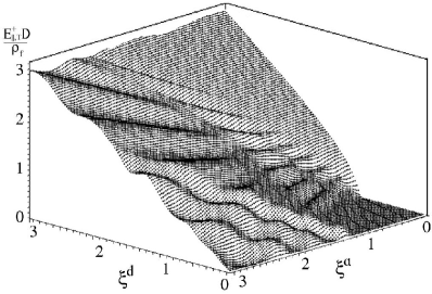
Figure 3: The longitudinal CVC $E^{dc+}_{\parallel,\textrm{T}}(\xi^{d},\xi^{a}),\Omega=0.2,g=100$, showing the Shapiro steps.

Now we consider the influence of a small ($\xi^{a}\ll 1$) $ac$ current density with a frequency $\omega$ on the CVC in the limit of very small temperatures ($g\ggg 1$). In this case the physics of the $dc$ response is quite different depending on the $\xi^{d}$ value with respect to the unity. If $\xi^{d}<1$, the vortex mainly (excluding very rare hops to the neighboring wells) localized at the bottom of the potential well where it experiences a small $\omega$-oscillations. The averaging of the vortex motion over the period of oscillations in this case cannot change the CVC which existed in the absence of the $ac$-drive.

If, however, $\xi^{d}>1$, then the vortex is in a running state with the internal frequency of oscillations $\omega_{i}=\sqrt{(\xi^{d})^{2}-1}$. If $\omega\neq\omega_{i}$, the CVC is changed only in the second-oder perturbation approach in terms of a small parameter $\xi^{a}\ll 1$ (as it was shown for the analogous resistively shunted Josephson junction problem KANVER ) because the CVC is not changed in the linear approximation in this case. However, for $\omega=\omega_{i}$ appears a problem of a synchronization of the running vortex oscillations at the $\omega_{i}$-frequency with the external driving frequency $\omega$. As a result, the average (over period of oscillations) vortex velocity is locked in with the $\omega$ in some interval of the $dc$ current density $\xi^{d}$ even within the frame of the first-order perturbation calculation. The width of this first synchronization step (or the so-called ”Shapiro step” in the resistively shunted Josephson junction problem) has been found in Ref. [ASLAR ] and the calculation in the spirit of this reference gives the boundaries of the $\xi^{d}$ where the step occurs as

$$(\xi^{d}_{\omega}-\xi^{a}/2\xi^{d})<\xi^{d}<(\xi^{d}_{\omega}+\xi^{a}/2\xi^{d}).$$ (53)

Here $\xi^{d}_{\omega}$ is the current density which gives $\omega_{i}=\sqrt{(\xi^{d}_{\omega})^{2}-1}=\omega$, i. e. $\xi^{d}_{\omega}=\sqrt{1+\omega^{2}}$. Then the size of the first Shapiro step on the CVC is $\xi^{a}/\xi^{d}_{\omega}$. In higher approximations (in terms of ($\xi^{a})^{m}$), where $m$ runs through all of the integers) the Shapiro steps on the CVC appear at the frequencies $\Omega=m\omega$ and $\Omega_{i}=m\omega_{i}$. The width of the $m$-th step at $\xi^{a}\rightarrow 0$ is proportional to $(\xi^{a})^{m}$, i. e. strongly decreases with $m$ increasing LIHUL .

In Fig. 3 we plot the longitudinal CVC $E^{dc+}_{\parallel,\textrm{T}}(\xi^{d},\xi^{a})$ showing the Shapiro steps. The plot in Fig. 3 looks like the similar curves discussed earlier VAN for the CVC of the microwave driven resistively shunted Josephson junction model at $T=0$ where the overall shape of the CVC and different behaviour of the two types of the Shapiro steps in adiabatic limit was explained. Our graph, in comparison with the curves of Ref. VAN , is smoothed due to the influence of a finite temperature. The longitudinal CVC $E^{dc+}_{\parallel,\textrm{T}}(\xi^{d},\xi^{a})$-dependence demonstrate several main features. First, in the presence of the microwave current the $dc$ critical current $\xi^{d}_{c}(\xi^{a})$ is a decreasing function of the $ac$ driving. The physical reason for such behaviour lies in the replacement of the $dc$ critical current by the total $dc+ac$ critical current. Second, with gradual $\xi^{a}$-increasing the zero-voltage step reduces to zero and all other steps appear. Such steps are common because they do not oscillate and spread over a $dc$-current range about twice the critical current $2\xi^{a}_{c}$. These steps are the steps of the first kind and they distort the CVC as like as relief bump with a concave shift from the ohmic line. With further $\xi^{a}$-increasing this relief bump shifts toward higher $\xi^{d}$-values. Below this range the steps of the second kind appear. These microwave current-induced steps oscillate rapidly and stay closely along the ohmic line VAN over a $dc$-current range $\xi^{d}\leq\xi^{a}-1$.

To summarize, we can determine three $(\xi^{d},\xi^{a})$-ranges where the CVC-behaviour is qualitatively different. For large $dc$ bias current densities $\xi^{a}+1<\xi^{d}$ the CVC asymptotically approaches the ohmic line without microwave induced steps. For an intermediate $dc$ current range $\xi^{a}-1<\xi^{d}<\xi^{a}+1$ CVC curve deviates from the ohmic line as a concave bump with the stable steps. For lower $dc$ current range $\xi^{d}<\xi^{a}-1$ the steps oscillate with microwave current along the ohmic line. With gradual $\Omega$-increasing the size of the steps increases whereas their number decreases.

V Nonlinear stationary ac response

V.1 Derivation of the impedance tensor

Using Eq. (11) we determine nonlinear (in the amplitudes $j^{ac}$, $j^{dc}$ and the frequency $\omega$) stationary $ac$ response as

$$\langle\mathbf{E}\rangle_{t}\equiv\langle\langle\mathbf{E}\rangle(t)-\langle\mathbf{E}\rangle_{0}^{\omega}\rangle=(nB/c)[\langle v_{x}\rangle_{t}\mathbf{y}-\langle v_{y}\rangle_{t}\mathbf{x}],$$ (54)

where $\langle\mathbf{E}\rangle_{0}^{\omega}=(nB/c)[-\langle v_{y}\rangle_{0}^{\omega}\mathbf{x}+\langle v_{x}\rangle_{0}^{\omega}\mathbf{y}]$ is time-independent part of $\langle\mathbf{E}\rangle(t)$ (see also Eqs. (26) and (29)), whereas $\langle v_{y}\rangle_{t}$ and $\langle v_{x}\rangle_{t}$ are time-dependent periodic parts of $\langle v_{y}\rangle(t)$ and $\langle v_{x}\rangle(t)$ which to become zero after averaging over a period $2\pi/\omega$ of the $ac$ cycle.

From Eqs. (13) and (54) we have

$$\langle E_{y}\rangle_{t}=(n\rho_{f}j_{c}/D)\sum_{\begin{subarray}{c}k=1\end{subarray}}^{\begin{subarray}{c}\infty\end{subarray}}(j^{ac})^{k}\textrm{Re}\{Z_{k}(\omega)e^{ik\omega t}\},$$ (55)

where

$$\begin{array}[]{ccr}Z_{k}(\omega)=\delta_{1,k}-i\psi_{k}(\omega)/(j^{ac})^{k},\\ \\ \psi_{k}(\omega)\equiv[F_{k}^{1}(\omega)-F_{k}^{-1}(\omega)],\end{array}$$ (56)

and $\delta_{1,k}$ is Kronecker‘s delta.

The dimensionless transformation coefficients $Z_{k}$ in Eq. (55) have a physical meaning of the $k$-th harmonic with frequency $\Omega_{k}\equiv k\omega$ in the $ac$ nonlinear $\langle E_{y}\rangle_{t}$ response. Equation (56) for $k=1$ yields

$$Z_{1}=1-i\psi_{1}/j^{ac},$$ (57)

and using Eqs. (54) and (55) we can express the nonlinear stationary $ac$ response on the $\omega$-frequency $E_{y1}^{ac}$, in terms of the nonlinear impedance $Z_{1}$ as

$$E_{y1}^{ac}=(\rho_{f}/D)(j^{ac}_{y}+\delta j^{ac}_{x})\textrm{Re}\{Z_{1}e^{i\omega t}\}.$$ (58)

If we put $Z_{1}\equiv\rho_{1}-i\zeta_{1}$, where $\rho_{1}$ and $\zeta_{1}$ are the dynamic resistivity and the reactivity, respectively, then Eq. (58) acquires form

$$E_{y1}^{ac}=(\rho_{f}/D)(j^{ac}_{y}+\delta j^{ac}_{x})\sqrt{\rho_{1}^{2}+\zeta_{1}^{2}}\cos(\omega t-\varphi_{1}),$$ (59)

where $\sqrt{\rho_{1}^{2}+\zeta_{1}^{2}}\equiv|Z_{1}|$ and $\varphi_{1}=\arctan(\zeta_{1}/\rho_{1})$ are the dimensionless amplitude and phase of the $ac$ response on the $j^{ac}_{Lx}=(j^{ac}_{y}+\delta j^{ac}_{x})\cos\omega t$ input.

Similarly, using Eq. (12) and (54), we can show that

$$\langle E_{x}\rangle_{t}=\rho_{f}j^{ac}_{x}\cos\omega t-\delta\langle E_{y}\rangle_{t},$$ (60)

and obtain $\omega$-frequency $ac$ response $E_{x1}^{ac}$ as

$$E_{x1}^{ac}=(\rho_{f}/D)\textrm{Re}\{e^{i\omega t}[(D-\delta^{2}Z_{1})j_{x}-\delta Z_{1}j_{y})]\}.$$ (61)

From Eqs. (58) and (61) follows that the complex amplitudes of the electric field $\textsl{{E}}_{1}$ and the current density $\textsl{{J}}=\textbf{j}e^{i\omega t}$ are connected by the relation $\textsl{{E}}_{1}=\hat{Z}\textsl{{J}}$, where $\hat{Z}$ is the frequency and $dc$ and $ac$ current amplitudes dependent impedance tensor

$$\hat{Z}(\omega)=\begin{pmatrix}Z_{xx}&Z_{xy}\\ Z_{yx}&Z_{yy}\end{pmatrix}=\frac{\rho_{f}}{D}\begin{pmatrix}D-\delta^{2}Z_{1}&-\delta Z_{1}\\ \delta Z_{1}&Z_{1}\end{pmatrix}.$$ (62)

It is relevant to remark the similarity of Eq. (30) and Eq. (62) from which follows that for the $ac$ response $Z_{1}$ plays the same role as $\nu_{0}^{\omega}$ for the $dc$ response.

However, the connection between $Z_{1}$ and the dynamical average pinning force $\langle\hat{F}_{px}\rangle_{t1}$ is more complex than the relation between $\nu_{0}^{\omega}$ and $\langle\hat{F}_{px}\rangle_{0}^{\omega}$ (see Eq. (28)). Taking into account the time dependence of the $\langle\hat{F}_{px}\rangle_{t1}$, it is easy to show that

$$\langle\hat{F}_{px}\rangle_{t1}=\textrm{Re}\{e^{i\omega t}[j^{ac}(Z_{1}-1)]\}.$$ (63)

Equation (63) gives physical interpretation of the $Z_{1}$ impedance and its structure may be compared with Eq. (28).

The real quantities $\mathbf{E}_{1}=\textrm{Re}\textbf{{E}}_{1}$ and $\mathbf{j}^{ac}=\textrm{Re}\textbf{{J}}$ are connected by the relation $\mathbf{E}_{1}=\hat{\rho}^{ac}\textbf{j}$, where the $ac$-response resistivity tensor is

$$\hat{\rho}^{ac}=\begin{pmatrix}\rho^{ac}_{xx}&\rho^{ac}_{xy}\\ \rho^{ac}_{yx}&\rho^{ac}_{yy}\end{pmatrix}.$$ (64)

Note that from Eqs. (58) and (61) follows that

$$\hat{\rho}^{ac}=\textrm{Re}\{\hat{Z}(\omega)e^{i\omega t}\}.$$ (65)

V.2 Longitudinal and transverse impedance responses

The experimentally measurable $ac$ resistive responses refer to coordinate system to the $ac$ current which directed, for simplicity, at the same angle $\alpha$ with respect to the $y$ axis as the $dc$ current (see Fig. 1). The longitudinal and transverse (with respect to the $ac$ current direction) components of the electric field $E^{ac}_{\parallel}$ and $E^{ac}_{\perp}$, are related to $E_{x}^{ac}(t)$ and $E_{y}^{ac}(t)$ by the same relations as for the $dc$ current (see Eqs. (37)). The latter is true for the relations between the experimentally observable longitudinal and transverse (with respect to the $\mathbf{j}^{ac}$ direction) magnetoresistivities $\rho^{ac}_{\parallel}=E^{ac}_{\parallel}/j^{a}$ and $\rho^{ac}_{\perp}=E^{ac}_{\perp}/j^{a}$ (where $j^{a}$ is $j^{ac}$ amplitude ($(j^{a})^{2}=(j^{ac}_{x})^{2}+(j^{ac}_{y})^{2})$. As a result we have

$$\rho^{ac}_{\parallel}=\textrm{Re}\{Z_{\parallel}e^{i\omega t}\},\quad\rho^{ac}_{\perp}=\textrm{Re}\{Z_{\perp}e^{i\omega t}\},$$ (66)

where

$$\begin{array}[]{crr}Z_{\parallel}=(\rho_{f}/D)[(D-\delta^{2}Z_{1})\sin^{2}\alpha+Z_{1}\cos^{2}\alpha],\\ \\ Z_{\perp}=(\rho_{f}/D)[\delta Z_{1}-D(1-Z_{1})\cos\alpha\sin\alpha].\\ \end{array}$$ (67)

Note, however, that the magnitudes of the $\rho^{ac}_{\parallel}$ and $\rho^{ac}_{\perp}$, given by Eqs. (66), in general (as in the case of $dc$ current), depend on the direction of the external magnetic field $\mathbf{B}$ along $z$ axis due to the $\delta=n\epsilon$ dependence of the $Z_{1}$ through the implicit dependence of $\psi_{1}(\omega)$ on the $j^{ac}$ and $j^{dc}$. In order to consider only $n$-independent magnitudes of the $\rho^{ac}_{\parallel}$ and $\rho^{ac}_{\perp}$ resistivities we should introduce the even (+) and odd (–) longitudinal and transverse magnetoresistivities with respect to magnetic field reversal in the form $\rho^{ac\pm}_{\parallel,\perp}(n)\equiv[\rho^{ac}_{\parallel,\perp}(n)\pm\rho^{ac}_{\parallel,\perp}(-n)]/2$.

Let us first separate $Z_{1}=1-i\psi_{1}/j^{ac}$ on the even $Z^{+}_{1}(n)=Z^{+}_{1}(-n)$ and the odd $Z^{-}_{1}(n)=-Z^{-}_{1}(-n)$ parts. If we assume $\psi_{1}(n)=\psi_{1}^{+}(n)+\psi_{1}^{-}(n)$, where $\psi_{1}^{\pm}(n)$ are the even and odd parts of $\psi_{1}(n)$ (i. e. $\psi_{1}^{\pm}(n)=[\psi_{1}(n)\pm\psi_{1}(-n)]/2$), then we have

$$\begin{array}[]{crr}Z^{+}_{1}(n)=1-inj_{c}[j_{y}\psi_{1}^{-}(n)-\delta j_{x}\psi_{1}^{+}(n)]/(j_{y}^{2}-\delta^{2}j_{x}^{2}),\\ \\ Z^{-}_{1}(n)=-inj_{c}[j_{y}\psi_{1}^{+}(n)-\delta j_{x}\psi_{1}^{-}(n)]/(j_{y}^{2}-\delta^{2}j_{x}^{2}).\end{array}$$ (68)

From now on, we can present Eqs. (67) in the form, similar to Eqs. (39) and  (40), with the only difference in the change of $\nu_{0}^{\omega\pm}$ for $Z_{1}^{\pm}$ and $\rho^{dc\pm}_{\parallel,\perp}$ for $Z^{\pm}_{\parallel,\perp}$. However, hereafter it will be suitable for us to present Eqs. (67) in another equivalent form

$$Z^{+}_{\parallel}=(\rho_{f}/D)[(D-\delta^{2}Z_{1}^{+})\sin^{2}\alpha+Z_{1}^{+}\cos^{2}\alpha],$$ (69)

$$Z^{-}_{\parallel}=(\rho_{f}/D)Z_{1}^{-}(\cos^{2}\alpha-\delta^{2}\sin^{2}\alpha),$$ (70)

$$Z^{+}_{\perp}=(\rho_{f}/D)[\delta Z_{1}^{-}-D(1-Z_{1}^{+})\sin\alpha\cos\alpha],$$ (71)

$$Z^{-}_{\perp}=(\rho_{f}/D)(\delta Z_{1}^{+}+DZ_{1}^{-}\sin\alpha\cos\alpha).$$ (72)

V.3 The Hall effect and the guiding of vortices in nonlinear AC response

Let us consider peculiarities of the $ac$ resistive responses in the investigated model due to the Hall effect. Experimentally, three types of measurements of the observed $ac$ resistive characteristics are possible in a prescribed geometry defined by a fixed value of the angle $\alpha$. First is $ac$ response measurements which investigate the dependence of observed $\rho_{\parallel,\perp}^{ac\pm}(\xi^{a}|\xi^{d},g)$ resistivities on the current density $\xi^{a}$ at fixed $dc$ current density $\xi^{d}$ and temperature $g$. Second is the dependence of $\rho_{\parallel,\perp}^{ac\pm}(g|\xi^{a},\xi^{d})$ on the temperature at fixed $\xi^{a}$ and $\xi^{d}$. Third, is the dependence of $\rho_{\parallel,\perp}^{ac\pm}(\xi^{d}|\xi^{a},g)$ on the $dc$ current density at fixed $\xi^{a}$ and $g$. The form of these dependences is governed by a geometrical factor - the angle $\alpha$ between the directions of the current density vector $\mathbf{j}(t)$ and the channels of the washboard pinning potential. There are two different forms of the dependence of $\rho_{\parallel,\perp}^{ac\pm}$ on the angle $\alpha$ (see formulas (69)-(72)). The first of these is the ”tensor” dependence, also present in the linear regimes (similar to the TAFF and FF regimes for formulas  (39) and (40)), which is external to the impedance $Z_{1}$ (see Eqs. (67)). The second is through the dependence of $Z_{1}$ on its arguments $\xi^{a}(\alpha)$ and $\xi^{d}(\alpha)$, which in the region of the transition from linear in $j^{ac}$ and $j^{dc}$ regimes (at $\xi^{a,d}\ll 1$ and $\xi^{a,d}\gg 1$) is substantially nonlinear.

First recall that in the absence of the Hall effect $(\epsilon=0)$ there exist only even (with respect to magnetic field inversion) impedances $Z^{+}_{\parallel,\perp}$ – the odd impedances $Z^{-}_{\parallel,\perp}$ are zero (see Eqs. (69)-(72)). The presence of nonzero value of $\epsilon$ leads not only to the appearance of a Hall contribution to the observed $ac$ responses on account of the even component $Z_{1}^{+}$ of the impedance $Z_{1}$, but also to the appearance of the odd component $Z_{1}^{-}$, which has a maximum in the region of the nonlinear transition from the one linear regime (at low $\xi^{a},\xi^{d}$ and $g\gg 1$) to another linear regime (at large $\xi^{a},\xi^{d}$ and arbitrary $g$) and is essentially equal to zero outside this transitional region (see Figs. 10, 11 in Ref. [3]). As a consequence, ”crossover” effects arise: contributions from $Z_{1}^{-}$ to effects due to $Z_{1}^{+}$, and vice versa; contributions from $Z_{1}^{+}$ to effects due to $Z_{1}^{-}$. Thus, in the even impedance $Z_{\perp}^{+}$ (see Eq. (71)), in addition to the main contribution created by the guiding of vortices and described by $Z_{1}^{+}$ there is present a Hall contribution arising due to $Z_{1}^{-}$. The expression for the odd impedance $Z_{\perp}^{-}$ (see Eq. (72)) contains, in addition to the Hall term arising due to $Z_{1}^{+}$, term due to $Z_{1}^{-}$.

V.4 AC response in LT geometries

In order to study a more simple form of Eqs. (69)-(72) we consider first the $L$ and $T$ geometries of the $ac$ response (see Fig. 1, insert).

In $L$ geometry $\alpha=\pi/2$ and $j_{L}^{ac}=\epsilon\xi^{a}$ does not depend on $n$ as well as $j_{L}^{dc}=\epsilon\xi^{d}$ for the $dc$ current. As a result, $\psi_{1,L}$ as well as $Z_{1,L}=1-i\psi_{1,L}/j_{L}^{ac}$ have $\psi_{1,L}^{-}=Z_{1,L}^{-}=0$. Finally, from Eqs. (69) follows

$$Z_{\parallel,L}^{+}=(\rho_{f}/D)[1+\delta^{2}(1-Z_{1,L}^{+})],\quad Z_{\parallel,L}^{-}=0,$$ (73)

$$Z_{\perp,L}^{+}=0,\quad Z_{\perp,L}^{-}=\delta(\rho_{f}/D)Z_{1,L}^{+}.$$ (74)

If we define $\rho_{\parallel,L}^{ac+}$ and $\zeta_{\parallel,L}^{ac+}$ as the resistivity and reactivity of $Z_{\parallel,L}^{+}$ impedance, respectively, by the relation $Z_{\parallel,L}^{+}=\rho_{\parallel,L}^{ac+}-i\zeta_{\parallel,L}^{ac+}$ we can show that

$$\begin{array}[]{ccr}\rho_{\parallel,L}^{ac+}=(\rho_{f}/D)(1-\epsilon\textrm{Im}\psi_{1,L}/\xi^{a}),\\ \\ \zeta_{\parallel,L}^{ac+}=-(\rho_{f}/D)\epsilon\textrm{Re}\psi_{1,L}/\xi^{a}.\\ \end{array}$$ (75)

Note that experimentally measured quantities $|Z_{\parallel,L}^{+}|$ and $\tan\varphi_{\parallel,L}=\zeta_{\parallel,L}^{ac+}/\rho_{\parallel,L}^{ac+}$ allow to obtain $\rho_{\parallel,L}^{ac+}$ and $\zeta_{\parallel,L}^{ac+}$ and to compare them with the theoretical formulas  (75). Similar calculations for $Z_{\perp,L}^{-}=\rho_{\perp,L}^{ac-}-i\zeta_{\perp,L}^{ac-}$ yield

$$\begin{array}[]{ccr}\rho_{\perp,L}^{ac-}=n(\rho_{f}/D)(\epsilon\xi^{a}-\textrm{Im}\psi_{1,L})/\xi^{a},\\ \\ \zeta_{\perp,L}^{ac-}=n(\rho_{f}/D)\textrm{Re}\psi_{1,L}/\xi^{a}.\\ \end{array}$$ (76)

In $T$ geometry (see insert in Fig. 1) $\alpha=0$, $j_{T}^{ac}=n\xi^{a}$ and $j_{T}^{dc}=n\xi^{d}$. In this case it follows from Eqs. (20)-(23) that $\psi_{1,T}(n)=-\psi_{1,T}(-n)$, i. e. $\psi_{1,T}$ is an odd function of $n$ and $\psi_{1,T}^{+}=0$. As a result,

$$Z_{1,T}^{+}=1-in\psi_{1,T}^{-}/\xi^{a},\quad Z_{1,T}^{-}=0.$$ (77)

Then from Eqs. (69)- (72) we have

$$Z_{\parallel,T}^{+}=(\rho_{f}/D)Z_{1,T}^{+},\quad Z_{\parallel,T}^{-}=0,$$ (78)

$$Z_{\perp,T}^{-}=(\rho_{f}/D)\delta Z_{1,T}^{+},\quad Z_{\perp,T}^{+}=0.\\$$ (79)

If $Z_{\parallel,T}^{+}=\rho_{\parallel,T}^{ac+}-i\zeta_{\parallel,T}^{ac+}$ and $Z_{\perp,T}^{-}=\rho_{\perp,T}^{ac-}-i\zeta_{\perp,T}^{ac-}$, then from Eqs. (78), (79) we obtain $Z_{\perp,T}^{-}=\delta Z_{\parallel,T}^{+}$ and

$$\rho_{\perp,T}^{ac-}=\delta\rho_{\parallel,T}^{ac+},\quad\zeta_{\perp,T}^{ac-}=\delta\zeta_{\parallel,T}^{ac+}.$$ (80)

From Eqs. (80) follows that that experimentally measured quantities satisfy the simple relations

$$|Z_{\perp,T}^{-}|=\epsilon|Z_{\parallel,T}^{+}|,\quad\tan\varphi_{\perp,T}^{-}=\tan\varphi_{\parallel,T}^{+}.$$ (81)

At last, from Eqs. (77) and (78) follows that $\rho_{\parallel,T}^{ac+}=(\rho_{f}/D)\rho_{1,T}^{ac+}$ and $\zeta_{\parallel,T}^{ac+}=(\rho_{f}/D)\zeta_{1,T}^{ac+}$, where

$$\begin{array}[]{ccr}\rho_{1,T}^{ac+}=1+n\rm{Im}\psi_{1,T}^{-}/\xi^{a},\\ \\ \zeta_{1,T}^{ac+}=n\rm{Re}\psi_{1,T}^{-}/\xi^{a},\quad\rho_{1,T}^{-}=\zeta_{1,T}^{-}=0.\\ \end{array}$$ (82)

V.5 The power absorption in AC response

In order to calculate the power absorbed per unit volume $\mathcal{\bar{P}}$ (and averaged over the period of an $ac$ cycle) we use the standard relation $\mathcal{\bar{P}}=(1/2)\textrm{Re}(\textbf{{E}}_{1}\cdot\textbf{{J}})$ where $\textbf{{E}}_{1}$ and J are the complex amplitudes of the $ac$ electric field and current density, respectively. Using Eqs. (62) and (67) we can show that

$$\mathcal{\bar{P}}=(j^{2}/2)\bar{\rho}\equiv(j^{2}/2)\textrm{Re}Z_{\parallel}.$$ (83)

After some algebra we obtain that

$$\bar{\rho}=(\rho_{f}/D)[D\sin^{2}\alpha+(1-D\sin^{2}\alpha)\textrm{Re}Z_{1}.$$ (84)

Taking into account that $Z_{1}\equiv 1-iG_{1}$, where $G_{1}\equiv\psi_{1}/j^{ac}$, we conclude that $\textrm{Re}Z_{1}=1-\textrm{Re}(iG_{1})=1+\textrm{Im}G_{1}$. Then from Eq. (84) we have

$$\bar{\rho}=(\rho_{f}/D)[1+(1-D\sin^{2}\alpha)\textrm{Im}G_{1}].$$ (85)

In the limit of $\epsilon\ll 1$ we obtain for $\bar{\rho}$ a more simple result

$$\bar{\rho}=\rho_{f}(1+\textrm{Im}G_{1}\cos^{2}\alpha),$$ (86)

which will be analyzed in detail in Sec. IV. F.

From Eq. (84) follows two simple results for $\bar{\rho}$ in $LT$ geometries

$$\bar{\rho}_{L}=(\rho_{f}/D)(D-\delta^{2}\textrm{Re}Z_{1L})=(\rho_{f}/D)(1-\epsilon\textrm{Im}\psi_{1L}/\xi^{a}),$$ (87)

$$\bar{\rho}_{T}=(\rho_{f}/D)\textrm{Re}Z_{1T}=(\rho_{f}/D)(1+n\textrm{Im}\psi_{1T}^{-}(n)/\xi^{a}).$$ (88)

Note that $\bar{\rho}_{L}$ and $\bar{\rho}_{T}$ in Eqs. (87) and (88) are equal to the expressions for the $\rho^{ac+}_{\parallel,L}$ and $\rho^{ac+}_{\parallel,T}$ given by Eqs. (75) and  (82), respectively.

V.6 AC impedance and power absorption at $\epsilon\ll 1$

Here we analyze the $ac+dc$ impedance dependences $Z^{\pm}_{\parallel}$ and $Z^{\pm}_{\perp}$ (see Eqs. (69)-(72)), with allowance for the small Hall effect $(\epsilon\ll 1)$. In this case Eqs. (69)-(72) become more simple and the expressions for $Z^{\pm}_{\parallel,\perp}$, out of terms of order $\epsilon^{2}\ll 1$, have the form

$$\begin{array}[]{crr}Z^{+}_{\parallel}=\rho_{f}(Z_{1}^{+}\cos^{2}\alpha+\sin^{2}\alpha),\\ \\ Z^{+}_{\perp}=\rho_{f}(Z_{1}^{+}-1)\sin\alpha\cos\alpha,\end{array}$$ (89)

$$\begin{array}[]{crr}Z^{-}_{\parallel}=\rho_{f}Z^{-}\cos^{2}\alpha,\\ \\ Z^{-}_{\perp}=\rho_{f}(\delta Z_{1}^{+}+Z_{1}^{-}\sin\alpha\cos\alpha),\end{array}$$ (90)

Here $Z_{1}^{\pm}$ can be obtained from relations

$$\begin{array}[]{ccr}Z_{1}=Z_{1}^{+}+Z_{1}^{-}=1-iG_{1}=\\ \\ 1-i(G_{1}^{+}+G_{1}^{-})=(1-iG_{1}^{+})-iG_{1}^{-},\end{array}$$ (91)

where $G_{1}\equiv\psi_{1}(j^{ac},j^{dc})/j^{ac}$ and $Z_{1}^{+}=(1-iG_{1}^{+}),Z_{1}^{-}=-iG_{1}^{-}$. In the case of a small Hall effect $(\epsilon\ll 1)$ the expression for even (+) and odd (–) components of $Z_{1}(\xi^{ac},\xi^{dc})$ (in terms of $G_{1}^{\pm}$) in the linear approximation in the parameter $\epsilon\tan\alpha\ll 1$ are equal, respectively, to

$$\begin{array}[]{crr}G_{1}^{+}=G_{1}(n\xi_{y}^{a},n\xi_{y}^{d}),+nR_{a}^{+}\delta\tan\alpha\\ \\ G_{1}^{-}=(-G_{1}^{+}+nR_{a}^{-})\delta\tan\alpha,\end{array}$$ (92)

$$R_{a}\equiv[(\partial\psi_{1}/\partial\xi_{y}^{a})+(j^{d}/j^{a})(\partial\psi_{1}/\partial\xi_{y}^{d})],$$ (93)

where $\psi_{1}=\psi_{1}(n\xi_{y}^{a},n\xi_{d}^{a})$, $j^{a}$ and $j^{d}$ are $ac$ and $dc$ current density values, and $R_{a}^{+}$, $R_{a}^{-}$ are even and odd parts of the $R_{a}$, respectively.

It is worth noticing that Eqs. (89) and  (90) have the same structure as Eqs. (46) and (47) for the $dc+ac$ response at $\epsilon\ll 1$. Actually, if we change $Z_{1}^{\pm}$ and $Z^{\pm}_{\parallel,\perp}$ in Eqs. (89) and (90) by $\nu_{0}^{\omega\pm}$ and $\rho^{dc\pm}_{\parallel,\perp}$, respectively, we obtain then Eqs. (46) and (47).

So all conclusions following the discussion about a structure of these equations can be repeated for the Eqs. (89) and (90).

It is interesting also to analyze an anisotropic power absorption in the limit of $\epsilon\ll 1$, given by Eq. (86) in the previous Section IV. E.

Let us put $G_{1}=G_{1}^{+}+G_{1}^{-}$, where $G_{1}^{\pm}$ are presented by Eqs. (92) and (93). In case where $\epsilon=0$, $G_{1}=G_{1}^{+}=G_{1}(n\xi_{y}^{a},n\xi_{y}^{d})=\psi_{1}(n\xi_{y}^{a},n\xi_{y}^{d})/n\xi_{y}^{a}$, where $\xi_{y}^{a}=\xi^{a}\cos\alpha$, $\xi_{y}^{d}=\xi^{d}\cos\alpha$ and

$$\bar{\rho}=\rho_{f}[1+\cos\alpha\cdot n\textrm{Im}\psi_{1}^{-}(n)/\xi^{a}],$$ (94)

Note, that Eq. (94) at $\alpha=0$ yields $\bar{\rho}=\bar{\rho}_{T}(\epsilon=0)$, where $\bar{\rho}_{T}$ is given by Eq. (88).

V.7 Linear ac response

Here we assume that $j=j^{dc}+j^{ac}e^{i\omega t}$ and the alternating current is small ($j^{ac}\ll 1$). There are three different ways to derive linear (in $j^{ac}$) impedance $Z_{1l}$ at arbitrary value of $j^{dc}$.

The first way is to use general expression for $Z_{1}(j^{ac},j^{dc})$ (see Eq. (57)) derived by the method of matrix continued fraction at arbitrary magnitudes of the $j^{ac}$ and $j^{dc}$. If we take into account that $\psi_{1}(j^{ac}=0)=0$, then it follows

$$Z_{1L}=\lim_{\begin{subarray}{c}j^{ac}\rightarrow 0\end{subarray}}Z_{1}=1-i(d\psi_{1}/dj^{ac})|_{j^{ac}=0}.$$ (95)

This method is the most general and powerful if we can calculate $Z_{1}(j^{ac},j^{dc})$.

The second way is to calculate $Z_{1l}$ by means of making the perturbation expansion of the $\langle r^{m}\rangle(t)$ (see Eq. (10)) in powers of $j^{ac}\ll 1$ in the form

$$\langle r^{m}\rangle_{t}=\langle r^{m}\rangle_{0}+\langle r^{m}\rangle_{1}+\dots,$$ (96)

where $\langle r^{m}\rangle_{1}=A_{m}(\omega)j^{ac}e^{i\omega t}$ and the subscript $"0"$ denotes the statistical averages in the absence of the $ac$ and the subscription $"1"$ the portion of the statistical average which is linear in the $ac$. Whereas the $\langle r^{m}\rangle_{0}$ satisfies Eq. (32), the complex amplitude $A_{m}(\omega)$ (for $m\geq 1$) can be presented (see details in subsection 5.5 of Ref. [CKW ]) in terms of the infinite scalar continued fraction $\tilde{S}_{m}(\omega)$ as

$$A_{1}(\omega)=2i\sum_{\begin{subarray}{c}n=1\end{subarray}}^{\begin{subarray}{c}\infty\end{subarray}}(-1)^{n}\prod_{\begin{subarray}{c}m=1\end{subarray}}^{\begin{subarray}{c}n\end{subarray}}S_{m}\tilde{S}_{m}(\omega),$$ (97)

where

$$\mathbf{\tilde{S}}_{m}(\omega)=\cfrac{1/2}{\frac{i\omega\hat{\tau}}{m}+ij^{dc}+\frac{m}{g}+\cfrac{1/4}{\frac{i\omega\hat{\tau}}{m+1}+ij^{dc}+\frac{m+1}{g}+...}}$$ (98)

and $\tilde{S}_{m}(\omega=0)=S_{m}$ (see also Eqs. (33) and (34)). Using Eq. (97) and taking into account that $A_{-1}(\omega)=-A^{\ast}_{1}(-\omega)$ we conclude that

$$\langle\sin\textsl{x}\rangle_{1}=(i/2)(\langle r\rangle_{1}-\langle r^{-1}\rangle_{1})=B(\omega)j^{ac}e^{i\omega t},$$ (99)

where $B(\omega)\equiv(i/2)[A_{1}(\omega)+A^{\ast}_{1}(-\omega)]$. Then from expressions for the $\langle v_{x}\rangle_{t1}$, taken at $j^{ac}e^{i\omega t}$, Eqs. (63) and (99) follows that dimensionless linear impedance is

$$Z_{1l}(\omega)=1-B(\omega).$$ (100)

At last, the third way to calculate the linear impedance gives an approximate analytical expression for $Z_{1l}(\omega)$ within the frames of the method of effective eigenvalue (see details in subsections 5.6 and 5.7 of Ref. [CKW ]). Following this approach we can express the dimensionless linear impedance in terms of the modified Bessel functions $I_{\nu}(z)$ as

$$Z_{1l}(\omega,g,j^{dc})=1-\frac{1}{2}[\frac{I_{1+\mu}(g)}{I_{\mu}(g)(\lambda+i\omega\hat{\tau})}+\frac{I_{1-\mu}(g)}{I_{-\mu}(g)(\lambda^{\ast}+i\omega\hat{\tau})}],$$ (101)

where

$$\lambda=I_{\mu}(g)I_{1+\mu}(g)/[2\int_{\begin{subarray}{c}0\end{subarray}}^{\begin{subarray}{c}g\end{subarray}}I_{\mu}(t)I_{1+\mu}(t)dt]$$ (102)

is an effective eigenvalue CKW and $\mu\equiv igj^{dc}$. It follows from Eqs. (101) and  (102) that at $\omega=0$

$$\begin{array}[]{ccr}Z_{1l}(\omega=0,g,j^{dc})=d[j^{dc}\nu_{0}(j^{dc})]/dj^{dc}=\\ \\ =1-\textrm{Re}[(2/I_{\mu}^{2}(g))\int_{\begin{subarray}{c}0\end{subarray}}^{\begin{subarray}{c}g\end{subarray}}I_{\mu}(t)I_{1+\mu}(t)dt],\\ \end{array}$$ (103)

where $\nu_{0}(j^{dc})$ is given by Eq. (35). Note also that the right-hand side of Eq. (103) is the exact expression for the dimensionless static differential resistivity in an analytical form. In the limit $j^{dc}=0$ from Eq. (103) follows the well-known result of Coffey and Clem¹¹ (see also Refs. [MART ; IZR ]). Actually, in this limit $\mu=0$ and

$$\lambda=\lambda^{\ast}=I_{0}(g)I_{1}(g)/[I_{0}^{2}(g)-1].$$ (104)

As a result

$$Z_{1l}(\omega,g,j^{dc}=0)\equiv Z_{1l}^{0}=\frac{\nu_{00}+(\omega\tau)^{2}+i\omega\tau(1-\nu_{00})}{1+(\omega\tau)^{2}},$$ (105)

where $\nu_{00}\equiv\nu_{0}(j^{dc}=0)=1/I_{0}^{2}(g)$ is the flux creep factorCLEM ; MART ; SD ; SSS and

$$\tau=\hat{\tau}/\lambda=\hat{\tau}[I_{0}^{2}(g)-1]/I_{0}(g)I_{1}(g)=\hat{\tau}(1-\nu_{00})[I_{0}(g)/I_{1}(g)]$$ (106)

is the characteristic relaxation time. If $Z_{1l}^{0}=\rho_{1l}^{0}-i\zeta_{1l}^{0}$, where $\rho_{1l}^{0}$ and $\zeta_{1l}^{0}$ are linear resistivity and reactivity in the absence of the $dc$ current, respectively, then from Eq. (105) (see also Eq. (2)) follows that

$$\rho_{1l}^{0}(\omega,g)=1-\frac{1-\nu_{00}}{1+(\omega\tau)^{2}},\qquad\zeta_{1l}^{0}=-\frac{\omega\tau(1-\nu_{00})}{1+(\omega\tau)^{2}}.$$ (107)

As expected, in the limit of zero temperature ($g\rightarrow\infty$) we have that $\nu_{00}\rightarrow 0,\tau\rightarrow\hat{\tau}$ and the results of Gittlemann and RosenblumGR (see also Eqs. (1) and (2)) are following from Eqs. (107).

V.8 Nonlinear impedance and harmonics response

Let us consider strong nonlinear effects in the $ac$ impedance of a sample subjected to a pure $ac$ drive dimensionless current density $\xi^{a}\cos\omega t$, where $\xi^{a}\equiv|\mathbf{j}^{ac}|/j_{c}$. In the following we will discuss the behavior of $(\xi^{d},~{}\xi^{a},~{}\Omega,~{}g)$-dependent impedance for simplicity in terms of the dimensionless $ac$ resistivity $\rho_{1}^{ac+}=\rho_{1}$ and reactivity $\zeta_{1}^{ac+}=\zeta_{1}$. As the angular $\alpha$-anisotropy in these responses is omitted, the experimental observation of the following dependences (see Figs. 4-8) can be carried out in fact by the measurement of the $\rho_{\parallel,T}^{ac+}$ and $\zeta_{\parallel,T}^{ac+}$ responses in T geometry (see Eqs. (77), (78), and the definition of the $Z_{\parallel,T}^{+}$). Figure 4 shows the dimensionless $ac$ resistivity $\rho_{1}$ and reactivity $\zeta_{1}$ versus $ac$ current density $\xi^{a}$ for different dimensionless frequencies $\Omega\equiv\omega\hat{\tau}$ at very low temperature (g=100).

As can be seen from the Fig. 4(a), when $\Omega$ is very small, the $\rho_{1}(\xi^{a})$ shows several characteristic features: a threshold $\xi^{a}_{c}$ value and a subsequent parabolic rise, above the threshold, with associated steplike structures. The threshold current density where a sudden increase in $\rho_{1}(\xi^{a})$ starts may be defined as critical current density $\xi_{c}^{a}$. The step height decreases with $\xi^{a}$ increasing. The reactivity $\zeta_{1}(\xi^{a})$ shows nearly periodic dynamic $2\pi$ -jumps of the vortex coordinate occurring as the drive current density $\xi^{a}$ is increased (see Fig. 4(b)). The curves in Figs. 4(a, b) look like the similar curves discussed earlier ZHAI for the nonlinear resistance and reactance of the purely $ac$-driven resistively shunted Josephson junction model at $T=0$ where the overall shape and phase slips of these curves at several dimensionless frequencies was explained in terms of the bifurcations in the time-dependent solution of the equation for the phase difference $\varphi$ across the junction MDC ; WOS . Analogous bifurcations of the dimensionless coordinate x versus dimensionless time $\hat{\tau/}\pi$ in our problem at $T=0$ can be calculated too.

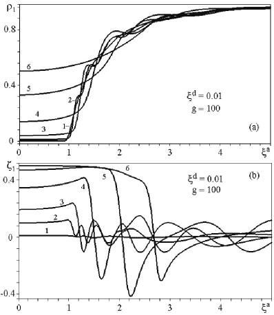
Figure 4: The $ac$ resistivity $\rho_{1}$ and reactivity $\zeta_{1}$ versus $\xi^{a}$ for various $\Omega=0.01(1),0.1(2),0.2(3),0.4(4),0.7(5),1(6),\xi^{d}=0.01,g=100.$

These bifurcations can cause sudden changes in $E_{y1}^{ac}(t)$ during one cycle of the alternating current and hence result in steps ZHAI .When $\Omega$ becomes large, both the threshold and steps in $\rho_{1}(\xi^{a})$ disappear and the amplitude of the x-jump in $\zeta_{1}(\xi^{a})$ becomes larger. Also, the x-jump moves to large values of $\xi^{a}$ and the spacing in $\xi^{a}$ between bifurcations becomes large which results in $\rho_{1}$ and $\zeta_{1}$ approaching unity. Because in our problem the abrupt $2\pi$-jumps of the dimensionless vortex coordinate x correspond to the overcoming by vortex of the potential barrier between two neighboring potential wells at nonzero temperature, our curves $\rho_{1}(\xi^{a})$ and $\zeta_{1}(\xi^{a})$, in comparison with the curves of Refs. [MDC ; WOS ] are smoothed due to the influence of a finite temperature.

It is worth noticing that the magnitude of $\rho_{1}(\xi^{a}|\Omega)$ in Fig. 4(a) at $\xi^{a}<1$ is approximately equal to a constant which progressively increases with $\Omega$ increasing. From a physical viewpoint it corresponds to the enhancement of power absorption with the growth of $\Omega$ due to the increasing of the viscous losses accordingly to GR (see Introduction) mechanism.

Now we consider the case when an $ac$ current driven sample is $dc$ current biased, i. e. the washboard pinning potential is tilted. In Fig. 5 we plot $\rho_{1}$ and $\zeta_{1}$ versus $\xi^{a}$ for various values of $\xi^{d}\equiv|\mathbf{j}^{dc}|/j_{c}$ at fixed dimensionless frequency $\Omega=0.1$ and very low temperatures (g=100). There are two regimes of behavior noticeable, corresponding to $\xi^{d}>\xi^{a}$ or $\xi^{a}<\xi^{d}$.

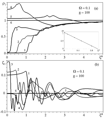
Figure 5: The $ac$ resistivity $\rho_{1}$ and reactivity $\zeta_{1}$ versus $\xi^{a}$ for various $\xi^{d}=0.01(1),0.5(2),0.8(3),1.5(4),3(5),10(6),g=100,\Omega=0.1$.

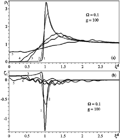
Figure 6: The $ac$ resistivity $\rho_{1}$ and reactivity $\zeta_{1}$ versus $\xi^{d}$ for various $\xi^{a}=0.01(1),0.1(2),0.5(3),0.7(4),1.5(5),10(6),g=100,\Omega=0.1$.

When $\xi^{d}$ is very small (for instance, $\xi^{d}=0.01$), the critical $ac$ current density $\xi_{c}^{a}(\xi^{d}=0.01)$ is found to be equal to $A\approx 1$(see Fig. 5(a)). When the $dc$ drive current density $\xi^{d}$ is smaller than $A$ (i. e. $0<\xi^{d}<A$), it can be seen that the $ac$ critical current density $\xi_{c}^{a}$ as a function of $\xi^{d}$ decreases and that both the step size and step rising pattern are changed. In the inset to Fig. 5(a) we plot the $\xi^{a}_{c}$ as a function of $\xi^{d}$ for $\Omega=0.1$. A linear fit $\xi_{c}^{a}=-\xi^{d}+A$ yields $A=1.02$. Note however that this $\xi_{c}^{a}(\xi^{d})$ function is weakly frequency-dependent.

When $\xi^{d}>A$, initially apparent jumps appear and with further increase of the $ac$ drive current density $\xi^{a}$, the $\rho_{1}$ begins to decrease with smoothed intermittence steps and eventually approaches the unity. This regime $(\xi^{a},\xi^{d})>\xi_{c}^{a}$ is rather interesting because it shows strong vortex-locking effects in the $ac$ impedance, similar to the Shapiro steps seen in the $dc$ CVC‘s. For very large values of $\xi^{d}$ ($\xi^{d}=10$), as expected, the effect of the microwave current density is negligible and the $ac$ dimensionless resistivity $\rho_{1}$ approaches the unity.

In the case of $ac$ reactivity $\zeta_{1}$, which is plotted in Fig. 5(b), the smoothed x-jump is not affected by the increase in the $dc$ current density $\xi^{d}$, however, the amplitude of this jump reduces substantially for larger values of $\xi^{d}$.

In Fig. 6 we plot $\rho_{1}$ and $\zeta_{1}$ versus $\xi^{d}$ for different $ac$ drive current densities $\xi^{a}=0.01,0.1,0.5,0.7,1.5,10$. It can be observed from the Fig. 6(a) that for all values of $\xi^{a}$, as $\xi^{d}$ increases, $\rho_{1}$ initially increases, reaches a maximum (very narrow and high for $\xi^{a}\lesssim 0.1$) and approaches unity eventually. On the other hand, $\zeta_{1}$, decreases for $\xi^{a}\lesssim 0.1$ slowly increases below $\xi^{d}\lesssim 1$ and then sharply decreases, having in the vicinity of $\xi^{d}\approx 1$ deep minimum, and then approaches to zero. So the occurrence of the x-jump can be seen clearly when $\xi^{d}$ is small, whereas large values of either $\xi^{a}$ or $\xi^{d}$ diminish the effect of the x-jumps.

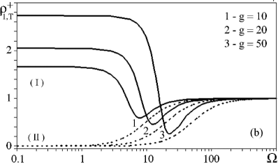
Figure 7: The frequency dependence of $\rho^{+}_{1,\textrm{T}}(\Omega)$ (b) for various $g$, (I) $\xi^{d}=1$ (solid lines), (II) $\xi^{d}=0$ (dotted lines).

In Fig. 6(a) the $\rho_{1}(\xi^{d})$ dependences demonstrate several main features. First, the curves, calculated at $\xi^{a}\ll 1$ show the progressive shrinking of the flux creep range (where the $\rho_{1}(\xi^{d})\lll 1$) with the $\xi^{a}$ increasing. If we define the $\xi^{d}_{c}(\xi^{a})$ as the dependence of the $dc$ critical current on the value of a small $ac$ driving, then we can show that $\xi^{d}_{c}\simeq 1-\xi^{a}$ at $\xi^{a}\ll 1$. The physical reason for such behavior is obvious. Second, the appearance of a high peak in $\rho_{1}(\xi^{d})$ near $\xi^{d}=1$ for $\xi^{a}\rightarrow 0$ can be simply explained from an examination of the $dc$ CVC curves, calculated at $\xi^{a}\rightarrow 0$. In this limit it is evident that a dynamic $dc$ resistivity (taken in the vicinity of the $\xi^{d}_{c}$), which equals to the derivative of the $dc$ CVC with respect to the $\xi^{d}$, is strongly enhanced at $T\rightarrow 0$. Third, taking into account an analogy between Brownian motion in a tilted periodic potential and continuous phase transitions USA , one can say that a threshold type phase transition in the vortex motion along the $x$-axis occurs between the ”localized” vortex state at $\xi^{d}<\xi^{d}_{c}(\xi^{a})$ and the ”delocalized” running state at $\xi^{d}>\xi^{d}_{c}(\xi^{a})$. If we consider only the linear impedance response (i. e. $Z_{1,L}(\omega)$ does not depend on $\xi^{a}$), this phase transition takes place at $\xi^{d}=1$ and at the $x$-point USA where $d^{2}U_{p}/dx^{2}=0$. Forth, as it was shown recently in RIEN , a strong enhancement of the effective diffusion coefficient D of an overdamped Brownian particle in a tilted washboard potential near the critical tilt may occur; that, in our case, $\textrm{D}(\xi^{d})$ may have a peak in the vicinity of $\xi^{d}=1$.

The consequences of the D-enhancement we analyze with the aid of Fig. 7 where the frequency dependence of $\rho_{1}(\Omega|\xi^{d}=0)$ (monotonic curves) and $\rho_{1}(\Omega|\xi^{d}=1)$ (nonmonotonic curves) calculated at $\xi^{a}=0$ for three different temperatures ($g=10,20,50$) are shown. The monotonic curves $\xi^{d}=0$ agree with the results of Coffey and Clem CLEM who, in fact, calculated the temperature dependence of the depinning frequency (introduced at $T=0$ in GR ) in a nontilted cosine pinning potential. In contrast to this monotonic behaviour, the nonmonotonic curves ($\xi^{d}$=1) demonstrate two characteristic features. First, an anomalous power absorption ($\rho_{1}\simeq 1,6\div 2,8$) at very low frequencies. Second, a deep minimum for the power absorption ($\rho_{1}\simeq 0,3\div 0,6$) at $T$-dependent $\Omega_{min}$. The appearance of this frequency- and temperature dependent minimum at $\xi^{d}=1$ may be related to the resonance activated reduction of the mean escape time of the Brownian particle due to an oscillatory variation of the pinning barrier height BOG .

At last we consider the frequency dependence of the k-th transformation coefficient amplitude, i.e. $|Z_{k}|(\Omega|j^{d},j^{a},g)$ taken at different values of the dc and ac current densities and inverse temperature. Here we point out only the summary of the $|Z_{k}|(\Omega)$ curves behaviour because a more detailed description of these results (interesting for applications) will be published elsewhere.

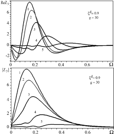
Figure 8: The third harmonic response $\textrm{Re}Z_{3}$ and $|Z_{3}|$ versus $\Omega$ for various $\xi^{a}=0.01(1),0.1(2),0.3(3),0.5(4),0.7(5),\xi^{d}=0.9,g=30.$

The main feature of the frequency dependence of the k-th harmonics is the appearance (see Fig. 8) of a pronounced maximum at $\xi^{d}=1$ for $\Omega_{max}=0.1$ in both $\textrm{Re}{Z_{k}(\Omega)}$ and $|Z_{k}|(\Omega)$ curves. The magnitude of the maximum is increasing with $\xi^{a}$-decreasing to zero and $g$-increasing to infinity. For example, the magnitudes of $\textrm{Re}{Z_{k}(\Omega_{max})}$ and $|Z_{k}|(\Omega_{max})$ are approximately equal to 20 for $k=3,4$ at $g=30$, $\xi^{d}=1$ and $\xi^{a}=0.01$.The emergence of this maximum and its growth with the temperature decreasing ($g\rightarrow\infty$) is related to the origin of a singularity of the $\delta^{\prime}(\omega)$-type in the $\Omega$-dependence of the linear impedance response of the overdamped shunted Josephson junction at T=0 and $\xi^{d}\lesssim 1$ AUR . Note also that $\textrm{Re}{Z_{k}(\Omega)}$ becomes negative in the vicinity of $\Omega_{max}$ which, in turn, is related to the origin of a similar singularity in the linear $Z_{1}(j^{dc}|{\Omega},g)$ response with the $\Omega$-increasing.

VI Conclusion

In conclusion, the considered exactly solvable two-dimensional model of the vortex dynamics is of great interest since a very rich physics is expected from combination of a strong $dc$ and $ac$ driving, arbitrary value of the Hall effect (note, that a big Hall effect was observed in YBCO HAR ), and the low temperature mediated vortex hopping (or running) in a washboard pinning potential. The obtained findings substantially generalize previous theoretical results in the field of the dc [2,3] and ac [11-13] stochastic approach to the study of the vortex dynamics in the washboard planar pinning potential. Experimental realization of this model in thin-film geometry HUTH ; OKS opens up a possibility for a variety of experimental studies of directed motion of vortices under ($dc+ac$)- driving simply by measuring longitudinal and transverse voltages. Experimental control of a frequency and value of the driving forces, damping, Hall constant, pinning parameters and temperature can be effectively provided.

While the discussion in this paper has been entirely in the context of nonlinear 2D pinning-mediated vortex dynamics, we are aware that obtained results are generic to all systems with a tilted washboard potential subjected to an ac driving. In this sense we are conscious of that physical explanation of our results should be supplemented by several new notions widely discussed. Here we mean notions of stochastic resonance BOG , resonance activation GAM , noise enhanced stability MAN which may be used not only for interpretation of our theoretical results, but on the contrary, the experimental verification of some predictions of these new approaches may be performed with the aid of the model under discussion.

It was shown also how pronounced nonlinear effects appear in the ac response and the linear response solutions are recovered from the nonlinear ac response in the weak ac current limit. An influence of a subcritical or overcritical dc current on the time-dependent stationary ac longitudinal and transverse resistive vortex response (on the frequency of an ac-driving $\Omega$) in terms of the nonlinear impedance tensor $\hat{Z}$ and a nonlinear ac response at $\Omega$-harmonics are studied. New analytical formulas for $2D$ temperature-dependent linear impedance tensor $\hat{Z}_{L}$ in the presence of a dc current which depend on the angle $\alpha$ between the current density vector and the guiding direction of the washboard PPP are derived and analyzed. Influence of $\alpha$-anisotropy and the Hall effect on the nonlinear power absorption by vortices is pointed out.

Up to now we have considered only the vortex motion problem. For the future experimental verification of our theoretical findings we should keep in mind that they may be applied directly only for thin-film superconductors in the form of naturally grown (for example, in the untwined a-axis oriented YBCO film TRA ) and artificially prepared washboard pinning structures HUTH . An application of our results for more general cases should take into account that they may be supplemented by consideration of the complex penetration length and the quasiparticle contribution in the way as it was made in the papers CLEM ; VORTEX .

References

- (1) G. Blatter, M. V. Feigelman, V. B. Geshkenbein, A. I. Larkin, and V. M. Vinokur, Rev. Mod. Phys. 66, 1125 (1994).
- (2) Y. Mawatari, Phys. Rev. B 56, 3433 (1997); Phys. Rev. B 59, 12033 (1999).
- (3) V. A. Shklovskij, A. A. Soroka, A. K. Soroka, Zh. Eksp. Teor. Fiz. 116, 2103 (1999), [JETP 89, 1138 (1999)].
- (4) V. A. Shklovskij and O. V. Dobrovolskiy, Phys. Rev. B 74, 104511 (2006).
- (5) V. V. Chabanenko, A. A. Prodan, V. A. Shklovskij, A. V. Bondarenko, M. A. Obolenskii, H. Szymczak, and S. Piechota, Physica C 314, 133 (1999).
- (6) H. Pastoriza, S. Candia, and G. Nieva, Phys. Rev. Lett. 83, 1026 (1999).
- (7) G. D’Anna, V. Berseth, L. Forro, A. Erb, and E. Walker, Phys. Rev. Lett. 81, 2530 (1998).
- (8) M. Huth, K. A. Ritley, J. Oster, H. Dosch, and H. Adrian, Adv. Funct. Mater. 12, 333 (2002).
- (9) O. K. Soroka, V. A. Shklovskij, and M. Huth, Phys. Rev. B 76, 014504 (2007).
- (10) J. I. Gittleman and B. Rosenblum, Phys. Rev. Lett. 16, 734 (1966).
- (11) M. W. Coffey and J. R. Clem, Phys. Rev. Let. 67, 386 (1991).
- (12) M. Martinoli, Ph. Fluckiger, V. Marsico, P. K. Srivastava, Ch. Leemann, and J. L. Gavilano, Physica B 165-166, 1163 (1990).
- (13) M. Golosovsky, Y. Naveh, and D. Davidov, Phys. Rev. B, 45, 7495 (1992).
- (14) W. T. Coffey, Yu. P. Kalmykov, and J. T. Waldron, The Langevin Equation, 2nd ed. (World Scientific, Singapore, 2004), Chap. 5.
- (15) W. T. Coffey, J. L. Dejardin, and Yu. P. Kalmykov, Phys. Rev. B, 62, 3480 (2000).
-
(16)
H. Risken, The Fokker-Planck Equation, 2nd ed. (Springer, Berlin, 1989).
- (17) G. N. Watson, Theory of Bessel Functions, 2nd ed. (Cambridge University Press, Cambridge, 1944), p. 46.
- (18) P. Reimann, C. Van den Broeck, H. Linke, P. Hanggi, J. M. Rubi, and A. Perez-Madrid, Phys. Rev. Lett. 87, 010602 (2001).
- (19) H. Kanter and F. L. Vernon, J. Appl. Phys., 43, 3174 (1972).
- (20) L. G. Aslamazov and A. I. Larkin, Zh. Eksp. Teor. Fiz., Pis‘ma Red. 9, 150 (1968) [JETP Letters 9, 87 (1969)].
- (21) K. K. Likharev and B. T. Ulrich, Systems with Josephson Contacts, (MSU, Moscow, 1978).
- (22) C. Vanneste et al., Phys. Rev. B 31, 4230 (1985).
- (23) Z. Zhai, P. V. Parimi, and S. Sridhar, Phys. Rev. B, 59, 9573 (1999).
- (24) J. McDonald and J. R. Clem, Phys. Rev. B, 56, 14723 (1997).
- (25) L. M. Xie, J. Wosik, and J. C. Wolfe, Phys. Rev. B. 54, 154949 (1996)
- (26) O. V. Usatenko and V. A. Shklovskij, J. Phys. A 27, 5043 (1994).
- (27) M. Boguna, J. M. Porra, J. Masoliver, and K. Lindenberg, Phys. Rev. E 57, 3990 (1998).
- (28) F. Auracher and Van Duzer, J. Appl. Phys., 44, 848 (1973).
- (29) J. M. Harris, Y. F. Yan, O. K. C. Tsui, Y. Matsuda, and N. P. Ong, Phys. Rev. Lett. 73, 1711 (1994).
- (30) L. Gammaitoni, P. Hanggi, P. Jung, and F. Marchesoni, Rev. Mod. Phys. 70, 233 (1998).
- (31) R. N. Mantegna and B. Spagnolo, Phys. Rev. Lett. 76, 563 (1996).
- (32) Z. Trajanovich, C. J. Lobb, M, Rajeswari, I. Takeuchi, C. Kwon, and T. Venkatesau, Phys. Rev. B 59, 14674 (1999),
- (33) E. Silva, N. Pompeo, S. Sarti, and C. Amabile, Vortex state microwave response in superconducting cuprate, ed. by B. P. Martins in Recent Development in Superconducting Research, (Nova Science, 2006), pp. 201-243.