Fate of the false monopoles: induced vacuum decay

Abstract

We study a gauge theory model where there is an intermediate symmetry breaking to a meta-stable vacuum that breaks a simple gauge group to a $U(1)$ factor. Such models admit the existence of meta-stable magnetic monopoles, which we dub false monopoles. We prove the existence of these monopoles in the thin wall approximation. We determine the instantons for the collective coordinate that corresponds to the radius of the monopole wall and we calculate the semi-classical tunneling rate for the decay of these monopoles. The monopole decay consequently triggers the decay of the false vacuum. As the monopole mass is increased, we find an enhanced rate of decay of the false vacuum relative to the celebrated homogeneous tunneling rate due to Coleman Coleman (1977a).

I Introduction

Semi-classical solutions with topologically non-trivial boundary conditions in relativistic field theory ’t Hooft (1974); Polyakov (1974, 1977) have the interesting property that they interpolate between two or more alternative translationally invariant vacua of the theory. For instance the exterior of a monopole or a vortex solution is a phase of broken symmetry while the interior of the object generically contains a limited region of unbroken symmetry (for more details and lucid expositions see Coleman (1977a) and Rajaraman (1982)). Most of the commonly studied solutions are topologically non-trivial, however non-trivial boundary conditions are not a guarantee of dynamical stability. In Preskill and Vilenkin (1993) for example a large number of such solutions are constructed in gauge field theories which are generically metastable. The skyrmion is also a classic example of a topologically non-trivial configuration that is unstable without the addition of fourth order Skyrme term Skyrme (1962); Gisiger and Paranjape (1998). All of the classically stable solutions (allowing for quantum metastabilty), are non-trivial time independent local minima of the effective action of the theory.

The metastability of such solutions can be of significant interest. The implied decay of the object would be accompanied by the change in phase of the system as a whole. In the context of cosmology this may imply a change in the cosmic history and determine the abundance of relic objects. On a more formal footing the question of metastability of vacua has gained considerable interest in the context of supersymmetric field theories where a non-supersymmetric phase is required on phenomenological grounds but such a phase is necessarily metastable on theoretical grounds Dine and Nelson (1993); Intriligator et al. (2006). In String Cosmology the de Sitter solution obtained is generically meta-stable Kachru et al. (2003) and its phenomenological viability depends on the tunneling rate being sufficiently slow.

Change in phase due to metastable topological objects is a generalisation of the following better known mechanism. When the effective potential of the theory possesses several local minima, all but the lowest minimum are quantum mechanically unstable. The so called false vacua are then liable to decay, even in the absence of topological objects, according to a rate given by a WKB-like formula studied earlier by Kobzarev et al. (1975) and provided an elegant and lucid footing by Coleman Coleman (1977b); Coleman and De Luccia (1980). The cases studied there concerned a transition between two translationally invariant vacua. The generic scenario of decay consists of spontaneous formation of a small bubble of true vacuum, which can then start growing by semi-classical evolution. In Minkowski space, the formation of one such bubble is sufficient to convert the phase of the system to the true vacuum. In the context of an expanding Universe, conversion of the entire Universe to the true vacuum would require formation of sufficiently large number of such bubbles at an adequate rate.

The existence of topological objects may provide additional sources of metastability. Phase transitions seeded by topological solutions were studied early in the works of Steinhardt (1981a); Hosotani (1983); Yajnik (1986); Yajnik and Padmanabhan (1987). An essential aspect of these studies is precisely the observations that there exist solutions with non-trivial boundary conditions which interpolate between two distinct minima of the effective potential. The importance of this alternative route to decay arises from the fact that it can be much more rapid than the spontaneous decay of a translationally invariant vacuum. Indeed, for some values of the parameters the decay induced by topological objects may require no tunneling and therefore would be very prompt in a context where the parameters are changing adiabatically, as for instance in the early Universe.

Obtaining a general formula characterising this kind of vacuum decay has been rather elusive although the ideas have been adequately explicated in Steinhardt (1981a); Hosotani (1983); Yajnik (1986); Yajnik and Padmanabhan (1987). More recently, the relevance of the mechanism has been demonstrated in specific examples, in Kumar and Yajnik (2009) for the mediating sector of a hidden sector scenario of supersymmetry breaking and in Kumar and Yajnik (2010) in a GUT model with O’Raifeartaigh type direct supersymmetry breaking. In this paper we explore a model that is amenable to an analytical treatment within the techniques developed in Coleman (1979). In doing so we provide a transparent model in which the generic expectations raised in Steinhardt (1981a); Hosotani (1983); Yajnik (1986); Yajnik and Padmanabhan (1987) can be realised and a specific formula can be derived.

We construct an $SU(2)$ gauge model with a triplet scalar field with two possible translationally invariant vacua, one with $SU(2)$ broken to $U(1)$ and the other with the original gauge symmetry intact. The former phase permits the existence of monopoles. By appropriate choice of potential for the triplet it can be arranged that the phase of unbroken symmetry is lower in energy and represents the true vacuum of the theory. The monopoles interpolate between the true vacuum and the false vacuum. For a wide range of the parameters, these monopoles are in fact classically stable. In previous work Steinhardt (1981a); Hosotani (1983) the dissociation of such monopoles was considered, varying the parameters of the theory to critical values where the monopoles were classically unstable due to infinite dilation. This can occur for example in the early Universe where the high temperature phase prefers one vacuum in which the system starts, but with adiabatic reduction in temperature, a different phase becomes more favorable. The Universe is then liable to simply roll over, by classical evolution, to the true vacuum.

It was however, overlooked that these monopoles are in fact unstable due to quantum tunneling well before the parameters reach their critical values. We dub such monopoles false monopoles. Working in the thin wall limit for the monopoles Steinhardt (1981a), we show that such monopoles undergo quantum tunneling to larger monopoles, which are then classically unstable by expanding indefinitely, consequently converting all space to the true vacuum, the phase of unbroken $SU(2)$ symmetry. Further, the formula we derive also recovers the regime of parameter space, within the thin wall monopole limit, where no tunneling is required for the decay but the monopole is simply classically unstable as previously treated Steinhardt (1981a); Hosotani (1983).

The rest of the paper is organised as follows. In section II we specify the model under consideration and the monopole ansatz along with the equations of motion. In section III we delineate the conditions under in which there should exist a metastable monopole solution with a large radius and a thin wall. We find the thin wall monopole solutions and also justify their existence. In section IV we use the thin wall approximation which permits a treatment of the solution in terms of a single collective coordinate, the radius $R$ of the thin wall. We argue that the monopole is unstable to tunneling to a new configuration of a much larger radius and we determine the existence of the instanton for this tunneling within the same thin wall approximation. In section V we determine the Euclidean action for this instanton, the so called bounce $B$ which determines the tunneling rate for the appearance of the large radius unstable monopole. In section VI we relate our findings to a previous study of classical monopole instability in supersymmetric GUT models. In section VII we discuss our results and compare our tunneling rate formula with that of the homogeneous bubble formation case without monopoles. We show that in addition to our tunneling rate being significantly faster, it also indicates a regime in which the monopoles become unstable, hence showing that the putative non-trivial vacuum indicated by the effective potential is in fact unstable.

II Unstable monopoles in a false vacuum

Consider an $SU(2)$ gauge theory with a triplet scalar field $\phi$ with the Lagrangian density given by

$$\mathcal{L}=-\frac{1}{4}F_{\mu\nu}^{a}F^{\mu\nu a}+\frac{1}{2}(D_{\mu}\phi^{a})(D^{\mu}\phi^{a})-V(\phi^{a}\phi^{a})$$ (1)

where

$$F_{\mu\nu}^{a}=\partial_{\mu}A_{\nu}^{a}-\partial_{\nu}A_{\mu}^{a}+e\epsilon^{abc}A_{\mu}^{b}A_{\nu}^{c},$$ (2)

and

$$D_{\mu}\phi^{a}=\partial_{\mu}\phi^{a}+e\epsilon^{abc}A_{\mu}^{b}\phi^{c}.$$ (3)

The potential we use is a polynomial of order $6$ in $\phi$ and may conveniently be written as

$$V(\phi)=\lambda\phi^{2}(\phi^{2}-a^{2})^{2}+\gamma^{2}\phi^{2}-\epsilon$$ (4)

where $\epsilon$ is defined so that the potential vanishes at the meta-stable vacua. The vacuum energy density difference is then equal to $\epsilon$. Such a potential was numerically analyzed by Steinhardt (1981b) as a toy model for the dissociation of monopoles. Here we obtain explicit analytical formulae for the quantum tunneling decay of the monopoles. The potential has a minimum at $\phi^{T}\phi=0$ which for $\gamma=0$ is degenerate with the manifold of vacua at $\phi^{T}\phi=a^{2}$. When we set $\gamma\neq 0$, we get a manifold of degenerate metastable vacua at $\phi^{T}\phi=\eta^{2}$ (where the exact value of the VEV, $\eta$, is calculable and satisfies $\eta\approx a$ for small $\gamma$), and the minimum at $\phi=0$ becomes the true vacuum. A plot of the potential for small $\gamma$ as a function of one of the components of $\phi$ is shown in figure 1. A supersymmetry breaking model Bajc and Melfo (2008) containing monopoles and a scalar potential similar to the one given in Eqn. (4) was studied in Kumar and Yajnik (2010).

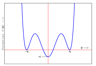
Figure 1: The potential $V(\phi)$ for $\gamma\neq 0$ as a function of one of the components of the field $\phi$, shifted by an additive constant so that $\phi=\eta$ has vanishing $V$ and the true vacuum has $V=-\epsilon$.

The manifold of vacua at $\phi^{T}\phi=\eta^{2}$ is topologically an $S^{2}$ and as spatial infinity is topologically also $S^{2}$, the appropriate homotopy group of the manifold of the vacua of the symmetry breaking $SU(2)\rightarrow U(1)$ is $\Pi_{2}(SU(2)/U(1))$ which is $\mathbf{Z}$. This suggests the existence of topologically non-trivial solutions of the monopole type which are classically stable. The presence of the global minimum at $\phi=0$ allows for the possibility that the monopole solution although topologically non-trivial, could be dynamically unstable.

A time independent spherically symmetric ansatz for the monopole can be chosen in the usual way as

$$\phi_{a} = \hat{r}_{a}\,h(r)$$

$$A_{\mu}^{a} = \epsilon_{\mu ab}\,\hat{r}_{b}\,\frac{1-K(r)}{er}$$

$$A_{0} = 0$$ (5)

where $\hat{r}$ is a unit vector in spherical polar coordinates The energy of the monopole configuration in terms of the functions $h$ and $K$ is

$$E(K,h)=4\pi\int_{0}^{\infty}dr\Big{(} \frac{(K^{\prime})^{2}}{e^{2}}+\frac{(1-K^{2})^{2}}{2e^{2}r^{2}}+\frac{1}{2}r^{2}(h^{\prime})^{2}$$

$$+K^{2}h^{2}+r^{2}V(h)\Big{)}$$ (6)

where derivatives with respect to $r$ are denoted by primes. The static monopole solution is the minimum of this functional and the ansatz functions satisfy the equations

$$h^{\prime\prime}+\frac{2}{r}h^{\prime}-\frac{2h}{r^{2}}K^{2}-\frac{\partial V}{\partial h} = 0$$ (7)

$$K^{\prime\prime}-\frac{K}{r^{2}}(K^{2}-1)-e^{2}h^{2}K = 0.$$ (8)

As $r\rightarrow\infty$ the function $h$ asymptotically approaches $\eta$ and is zero at $r=0$ from continuity requirements. On the other hand, $K$ approaches zero at spatial infinity so that the gauge field decreases as $1/r$, and $K=1$ at $r=0$.

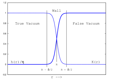
Figure 2: The monopole profile under the thin wall approximation.

III Thin walled monopoles

When the difference between the false and true vacuum energy densities $\epsilon$ is small, the monopole can be treated as a thin shell, the so called thin wall approximation. Within this approximation, the monopole can be divided into three regions as shown in figure 2. There is a region of essentially true vacuum extending from $r=0$ upto a radius $R$. At $r=R$, there is a thin shell of thickness $\delta$ in which the field value changes exponentially from the true vacuum to the false vacuum. Outside this shell the monopole is essentially in the false vacuum, and so we have

$$h\approx 0\,,\,K\approx 1\qquad\qquad r<R-\frac{\delta}{2}$$

$$h\approx\eta\,,\,K\approx 0\qquad\qquad r>R+\frac{\delta}{2}$$

$$0<h<\eta\,,\,0<K<1\qquad\qquad R-\frac{\delta}{2}\leq r\leq R+\frac{\delta}{2}$$ (9)

where $\delta$ is a length corresponding to the mass scale of the symmetry breaking. As we shall see in section IV, describing the monopole in this way allows us to study the dynamics in terms of just one collective coordinate $R$. The energy of the monopole then becomes a simple polynomial in $R$. Furthermore, due to the spherical symmetry, $R$ is a function of time alone and so the original field theoretic model in $3+1$ dimensions reduces to a one-dimensional problem involving $R(t)$.

We now proceed to elucidate the existence of monopole solutions which have the thin wall behavior described in the previous subsection. Redefining the couplings appearing in the potential (4) in terms of a mass scale $\mu$ and expressing $\phi$ in terms of the profile function $h(r)$, we have

$$V=\frac{\tilde{\lambda}}{\mu^{2}}h^{2}\big{(}h^{2}-\mu^{2}\tilde{a}^{2}\big{)}^{2}+\tilde{\gamma}^{2}\mu^{2}h^{2}-\epsilon$$ (10)

where a tilde over a variable indicates that it is dimensionless. The vacuum expectation value of $\phi$ or $h$ then becomes $\tilde{\eta}\mu$, where

$$\tilde{\eta}=\sqrt{\frac{2\tilde{a}^{2}}{3}+\frac{\sqrt{\tilde{a}^{4}\tilde{\lambda}^{2}-3\tilde{\gamma}^{2}\tilde{\lambda}}}{3\tilde{\lambda}}}.$$ (11)

The expression for $V$ can be rearranged as

$$V=\Big{(}\big{(}\tilde{\lambda}\tilde{a}^{4}+\tilde{\gamma}^{2}\big{)}\mu^{2}-2\tilde{\lambda}\tilde{a}^{2}h^{2}\Big{)}h^{2}+O(h^{6}).$$ (12)

The condition that $V$ is approximately quadratic in $h$ is given by

$$\frac{h^{2}}{\mu^{2}}<<\frac{\tilde{\lambda}\tilde{a}^{4}+\tilde{\gamma}^{2}}{2\tilde{\lambda}\tilde{a}^{2}}.$$ (13)

When the above condition is satisfied, $\partial V/\partial h$ is linear in $h$. The equation of motion for $h$ given in equation (8) can then be written as

$$h^{\prime\prime}+\frac{2}{r}h^{\prime}-\frac{2h}{r^{2}}-k^{2}h=0$$ (14)

where $k^{2}=(\tilde{\lambda}\tilde{a}^{4}+\tilde{\gamma}^{2})\mu^{2}$ and $K$ has been set to unity. Equation (14) has the form of the modified spherical Bessel equation whose general form is

$$z^{2}w^{\prime\prime}+2zw^{\prime}-[z^{2}+l(l+1)]w=0$$ (15)

for a function $w(z)$. The primes in the above equation denote derivatives with respect to $z$ and equation (14) is obtained from (15) with $l=1$.

The solution of equation (14) is

$$h(r)=C\Big{(}\frac{I_{3/2}(kr)}{\sqrt{kr}}\Big{)}=Ci_{1}(kr)$$ (16)

where $I_{J}$ is the modified Bessel function of the first kind of order $J$, $i_{n}$ is the modified spherical Bessel function of the first kind of order $n$, and $C$ is an arbitrary constant. The function $i_{1}(kr)\sim e^{kr}/(kr)$ for $kr\gg 1$ and is linear in $kr$ for small $kr\ll 1$. If we choose $C=e^{-k\xi}$ with arbitrarily large $k\xi$, we see that we can keep Eqn. (13) satisfied and hence stay with the linear equation for $h(r)$ for arbitrarily large $kr$.

The existence of the particular solution with $h(r)=\eta$ at $r=\infty$ can be proven using an argument similar to Coleman’s, where he proved in a somewhat different context, the existence of a thin wall instanton, Coleman (1977b). We can reinterpret the equation for the monopole profile, Eqn. (7), as describing the motion of a particle whose position is denoted by $h(r)$ where $r$ is now interpreted as a time coordinate. The particle moves in the presence of friction with a time dependent Stokes coefficient given by the second term in Eqn. (7) and a time dependent force given by the third term in Eqn. (7) (setting $K=1$), both of which are singular at $r=0$. The particle also moves in the potential $-V(h)$, obtained by inverting the potential Eqn. (4), as shown in figure 3. The particle must start at $h=0$ with a finite velocity and must reach $h=\eta$ as $r\rightarrow\infty$.

We prove the existence of the solution that achieves $h=\eta$ at $r=\infty$ by proving that initial conditions can be chosen so that the particle can undershoot or overshoot $h=\eta$ for $r\rightarrow\infty$, depending on the choice of the initial velocity. Then by continuity there must exist an appropriate initial condition for which the particle exactly achieves $h=\eta$ at $r\rightarrow\infty$.

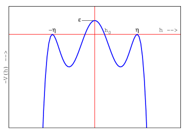
Figure 3: The scalar potential $-V(h)$ which is the Euclidean space equivalent of the potential given in (4). The potential has zeroes at $h=h_{0}$ and $h=\eta$.

In the following, we will assume that $K=1$ is always a good approximation. Indeed, in Eqn, (7) the term dependent on $K$ is negligible for large $r$ no matter the value of $K$, while for small $r$, $K=1$ is a reasonable approximation. On the other hand, Eqn. (8) for $K$, critically depends on the value of $h(r)\neq 0$, especially for large $kr$. In that sense, the function $h(r)$ does not depend strongly on $K(r)$ whereas, $h(r)$ drives the behaviour of $K(r)$.

III.1 Overshoot

The existence of the overshoot can be proven by taking a sufficiently small value of $C$. As explained earlier, $C$ can be chosen small enough so that Eqn.(13) is valid even for large $kr$, hence the equation remains linear. If $kr$ is large enough, the friction term $(2/r)h^{\prime}$ and the term $(2/r^{2})h$ in the equation of motion can be neglected in any further evolution and the evolution can be thought of as conservative. Thus with such a choice of $C$, $h$ increases to $\tilde{h}<h_{0}$ at a large value of $kr$ according to the linearised equation ($h_{0}$ is the zero crossing point of the potential, see Fig. (3)). The motion from then onwards is frictionless. The particle has an energy $E>0$ at $h=\tilde{h}$, thus it’s energy is still positive when it reaches $h=\eta$. As a result, it overshoots to $h>\eta$.

III.1.1 Technical details

III.2 Undershoot

To prove the existence of the undershoot, we start with the full equation for $h(r)$:

$$h^{\prime\prime}+\frac{2}{r}h^{\prime}-\frac{2}{r^{2}}h-\frac{\partial V}{\partial h}=0$$ (17)

which after multiplying both sides by $h^{\prime}$ can be rewritten as

$$\frac{d}{dr}\Big{(}\frac{1}{2}(h^{\prime})^{2}-V(h)\Big{)} = -2h^{\prime}\Big{(}\frac{h^{\prime}}{r}-\frac{h}{r^{2}}\Big{)},$$ (18)

$$= -2h^{\prime}\big{(}\frac{h}{r}\big{)}^{\prime}.$$ (19)

The quantity on the left hand side of Eqn. (18) can be thought of as the time derivative of the energy $E$. In the linearised regime, it is easy to show that the right hand side is strictly negative for all $r$. It starts with a value of zero at $r=0$ and decreases essentially exponentially for large $kr$. We can chose $C$, which amounts to choosing the initial velocity so that $h$ evolves according to the linearised equation until $kr$ can be taken to be large. However, in contrast to the case of the undershoot, we now require that $E$ becomes negative. This means that the value of $C$ is taken larger than in the case of the overshoot. $E$ is made up of two terms, the kinetic term which is positive semi-definite, and the potential term which becomes negative for $h>h_{0}$. We impose conditions on the parameters so that $E$ becomes negative and consequently $h>h_{0}$ within the linearised regime. Now if $kr$ is large enough, as before, the subsequent evolution will be conservative and since the total energy is negative, the subsequent evolution will never be able to overcome the hill at $h=\eta$ and the particle will undershoot.

III.3 Technical details

To make the previous arguments more precise and rigorous, we note that when the condition Eqn. (13) is satisfied, the linear regime is valid and $V(h)$ is approximately quadratic in $h$, ie. $-V(h)\approx\epsilon-(1/2)k^{2}h^{2}$ and the equation of motion for $h$ is approximately

$$\frac{d}{dr}\Big{(}\frac{1}{2}(h^{\prime})^{2}+\epsilon-\frac{1}{2}k^{2}h^{2}\Big{)}=-2h^{\prime}\Big{(}\frac{h^{\prime}}{r}-\frac{h}{r^{2}}\Big{)}.$$ (20)

Using the properties of $i_{1}(kr)$ we can compute $E$ in the linear regime, we find for large $kr$

$$E\approx\epsilon-\frac{k^{2}C^{2}e^{2kr}}{4(kr)^{3}}$$ (21)

which can be evidently taken to be positive or negative by simply choosing the value of $C$. Then in the subsequent evolution, where we can no longer rely on the linear evolution, the right hand side has two competing terms, the friction term, which only reduces the energy and the time dependent force term which tries to increase it. The change in the energy for evolution between $r_{0}$ and $r_{f}$ is given by the integral of the right hand side.

III.3.1 Overshoot

For the case of the overshoot, we use the expression Eqn. (19) which gives

$$\Delta E=-2\int_{r_{0}}^{r_{f}}\,dr\,h^{\prime}\big{(}\frac{h}{r}\big{)}^{\prime}.$$ (22)

Assuming that $h^{\prime}(r)$ is positive, we will find an estimate for $h^{\prime}(r)<v$. Then

$$|\Delta E| < 2v\left|\int_{r_{0}}^{r_{f}}\,dr\,\big{(}\frac{h}{r}\big{)}^{\prime}\right|$$ (23)

$$= 2v\left|\left(\frac{h(r_{f})}{r_{f}}-\frac{h(r_{0})}{r_{0}}\right)\right|$$ (24)

$$< 2v\left|\left(\frac{\eta}{r_{f}}-\frac{h(r_{0})}{r_{0}}\right)\right|$$ (25)

where we replaced $h(r_{f})$ with $\eta$ since that is its largest possible value. As long as $v$ is well behaved, as $r_{0}\to\infty$, $r_{f}>r_{0}$ thus the first term vanishes, while the second term can be made small by choosing the value of $C$ to be arbitrarily small. Thus we see that $\Delta E\to 0$ and therefore the change in the energy is arbitrarily small. Thus we necessarily obtain an overshoot since at $r=r_{\eta}$ such that $h(r_{\eta})=\eta$, $V(\eta)=0$, hence the particle has a positive kinetic energy giving an overshoot.

To get the value of $v$, we use Eqn. (18)

$$\frac{d}{dr}\Big{(}\frac{1}{2}(h^{\prime})^{2}-V(h)\Big{)} = -2h^{\prime}\Big{(}\frac{h^{\prime}}{r}-\frac{h}{r^{2}}\Big{)},$$ (26)

$$< 2\frac{hh^{\prime}}{r^{2}}<\frac{(h^{2})^{\prime}}{r_{0}^{2}}.$$ (27)

Integrating both sides from $r_{0}$ to $r_{f}$ yields

$$(h^{\prime}(r_{f}))^{2} < 2\left(\frac{1}{r_{0}^{2}}\left(h^{2}(r_{f})-h^{2}(r_{0})\right)\right.$$ (28)

$$+ \left.V(h(r_{f}))-V(h(r_{0}))+\frac{1}{2}(h^{\prime}(r_{0}))^{2}\right).$$ (29)

Thus $v^{2}$ is given by

$$v^{2} = 2\left(\frac{1}{r_{0}^{2}}\left(\eta^{2}-h^{2}(r_{0})\right)\right.$$ (30)

$$+ \left.\sup\left|V(h(r_{f}))-V(h(r_{0}))\right|+\frac{1}{2}(h^{\prime}(r_{0}))^{2}\right)$$ (31)

which is a bounded function of $r_{0}$.

III.3.2 Undershoot

To prove the undershoot we use the expression Eqn. (18) which gives

$$\Delta E=-2\int_{r_{0}}^{r_{f}}\,dr\,\frac{{h^{\prime}}^{2}}{r}+2\int_{r_{0}}^{r_{f}}\,dr\,\frac{{h^{\prime}}h}{r^{2}}.$$ (32)

Integrating the second term by parts we obtain

$$2\int_{r_{0}}^{r_{f}}\,dr\,\frac{{h^{\prime}}h}{r^{2}} = \int_{r_{0}}^{r_{f}}\,dr\,\left(\frac{h^{2}}{r^{2}}\right)^{\prime}+\int_{r_{0}}^{r_{f}}\,dr\,\left(\frac{2h^{2}}{r^{3}}\right)$$ (33)

$$< \left.\left(\frac{h^{2}}{r^{2}}\right)\right|_{r_{0}}^{r_{f}}-\eta^{2}\left.\left(\frac{1}{r^{2}}\right)\right|_{r_{0}}^{r_{f}}$$ (34)

where we obtain the inequality using the fact that we are only interested in the region $h\leq\eta$.

We now prove that this contribution to the energy cannot be sufficient push $h$ to $h>\eta$. We take $r_{0}$ to be the value of $r$ as described after Eqn. (19), where the energy becomes negative within the linearised regime with $kr_{0}\gg 1$. We now assume there exists a value $r_{f}\equiv r_{\eta}$ for which $h(r_{\eta})=\eta$. Then

$$\Delta E < -2\int_{r_{0}}^{r_{\eta}}\,dr\,\frac{{h^{\prime}}^{2}}{r}+\left.\left(\frac{h^{2}}{r^{2}}\right)\right|_{r_{0}}^{r_{\eta}}-\eta^{2}\left.\left(\frac{1}{r^{2}}\right)\right|_{r_{0}}^{r_{\eta}}$$ (35)

$$< \frac{\eta^{2}}{r_{\eta}^{2}}-\frac{h^{2}(r_{0})}{r_{0}^{2}}-\eta^{2}\left(\frac{1}{r_{\eta}^{2}}-\frac{1}{r_{0}^{2}}\right)$$ (36)

$$= \frac{\eta^{2}-h^{2}(r_{0})}{r_{0}^{2}}$$ (37)

which is an upper bound to the energy that can be added to the particle. But now it is easy to see that this is insufficient for $kr_{0}$ large enough. Indeed the energy of the particle at $r=r_{0}$ is obtained, via the linear regime, by Eqn. (21)

$$E\approx\epsilon-\frac{k^{2}C^{2}e^{2kr}}{4(kr)^{3}}\rightarrow\epsilon-k\frac{h^{2}(r_{0})}{r_{0}}.$$ (38)

This expression is negative. Furthermore, if $kr_{0}$ is large enough, we will see that $\Delta E$ cannot provide enough energy to increase $E$ to zero, giving a contradiction to the existence of $r_{\eta}$. To see this, we would require $|E|>\Delta E$ ie.

$$k\frac{h^{2}(r_{0})}{r_{0}}-\epsilon>\frac{\eta^{2}-h^{2}(r_{0})}{r_{0}^{2}}.$$ (39)

The linear approximation assumes $h(r_{0})\ll\eta$, hence we get

$$\frac{kh^{2}(r_{0})}{r_{0}}-\frac{\eta^{2}}{r_{0}^{2}}>\epsilon$$ (40)

reorganizing the terms, which for small enough $\epsilon$ simply implies

$$h^{2}(r_{0})kr_{0}>\eta^{2}.$$ (41)

Thus we get the the inequality sandwich

$$\frac{\eta^{2}}{kr_{0}}<h^{2}(r_{0})<\eta^{2}.$$ (42)

Using $h(r_{0})\approx Ce^{kr_{0}}/2kr_{0}$ we can choose

$$C=\frac{\eta 2kr_{0}}{e^{kr_{0}}r_{0}^{1/4}}$$ (43)

which gives

$$\frac{\eta^{2}}{kr_{0}}<\frac{\eta^{2}}{\sqrt{kr_{0}}}<\eta^{2}.$$ (44)

It is obvious that for large enough $kr_{0}$ this is easily satisfied. Thus we have established the existence of a choice of $C$ or initial velocity which contradicts the existence of $r_{\eta}$.

IV Collective coordinate and the instantons

The potential $V(\phi)$ given in (4) can be normalized so that the energy density of the metastable vacuum is vanishing whereas the energy density of the true vacuum is $-\epsilon$. By making use of the thin-wall approximation, the expression for the total energy in the static case given in (6) can be expressed as

$$E=4\pi \Bigg{[} \int_{0}^{R-\frac{\delta}{2}}dr\,r^{2}V(h)+\int_{R+\frac{\delta}{2}}^{\infty}dr\,\frac{1}{2e^{2}r^{2}}$$ (45)

$$+ \int_{R-\frac{\delta}{2}}^{R+\frac{\delta}{2}}dr\,\Big{(}\frac{(K^{\prime})^{2}}{e^{2}}+\frac{(1-K^{2})^{2}}{2e^{2}r^{2}}$$

$$+ \frac{1}{2}r^{2}(h^{\prime})^{2}+K^{2}h^{2}+r^{2}V(h)\Big{)}\Bigg{]}.$$

In the above expression, we have made use of the fact that $V(h)$ is zero for $r>R+\frac{\delta}{2}$, $K=1$ for $r<R-\frac{\delta}{2}$, $K=0$ for $r>R+\frac{\delta}{2}$, and that both the derivative terms and the term $K^{2}h^{2}$ are non-zero only when $R-\frac{\delta}{2}<r<R+\frac{\delta}{2}$. Since $\delta$ is small, the first integral on the right hand side of (45) gives $-\alpha R^{3}$ where $\alpha=4\pi\epsilon/3$ because $V(h)=-\epsilon$ in the domain of integration. The second integral gives $C/R$ where $C=2\pi/e^{2}$. The third integral is due to the energy of the wall and can be written as $4\pi\sigma R^{2}$ where $\sigma$ is the surface energy density of the wall given by

$$\sigma = \frac{1}{R^{2}}\int_{R-\frac{\delta}{2}}^{R+\frac{\delta}{2}}dr\,\Big{(}\frac{(K^{\prime})^{2}}{e^{2}}+\frac{(1-K^{2})^{2}}{2e^{2}r^{2}}$$ (46)

$$+ \frac{1}{2}r^{2}(h^{\prime})^{2}+K^{2}h^{2}+r^{2}V(h)\Big{)}.$$

We can thus write the total energy of the monopole as

$$E(R)=-\alpha R^{3}+4\pi\sigma R^{2}+\frac{C}{R}.$$ (47)

This function is plotted in figure 4. There is a minimum at $R=R_{1}$ and this corresponds to the classically stable monopole solution. This solution has a bubble of true vacuum in its core and the radius $R_{1}$ of this bubble is obtained by solving $dE/dR=0$. However, this monopole configuration can tunnel quantum mechanically through the finite barrier into a configuration with $R=R_{2}$ where $E(R_{1})=E(R_{2})$. Once this occurs, the monopole can continue to lose energy through an expansion of the core since the barrier which was present at $R_{1}$ is no longer able to prevent this.

Figure 4: The function $E(R)$ plotted versus bubble radius. The classically stable monopole solution has $R=R_{1}$. This solution can tunnel quantum mechanically to a configuration with $R=R_{2}$ and then expand classically.

We now proceed to determine the action of the instanton describing the tunneling from $R=R_{1}$ to $R=R_{2}$. In the thin wall approximation, the functions $h$ and $K$ can be written as

$$h = h(r-R)$$

$$K = K(r-R)$$ (48)

and the exact forms of the functions $h$ and $K$ will not be required in the ensuing analysis. The only requirement is that both $h$ and $K$ change exponentially when their argument $(r-R)$ is small. An example of a function with this type of behaviour is the hyperbolic tangent function. The time derivative of $\phi$ can be written as

$$\dot{\phi}^{a}=\hat{r}_{a}\frac{dh}{dR}\dot{R}.$$ (49)

From (48), since $(dh/dR)^{2}=(dh/dr)^{2}$, we have

$$\frac{1}{2}\dot{\phi}^{a}\dot{\phi}^{a}=\frac{1}{2}\left(\frac{dh}{dR}\right)^{2}\dot{R}^{2}=\frac{1}{2}\left(\frac{dh}{dr}\right)^{2}\dot{R}^{2}.$$ (50)

Similarly,

$$\dot{A}_{\mu}^{a}=\epsilon_{\mu ab}\hat{r}_{b}\left(\frac{-1}{er}\right)\frac{dK}{dR}\dot{R}$$ (51)

and

$$\frac{1}{4}\dot{A}_{\mu}^{a}\dot{A}_{\mu}^{a}=\frac{1}{2e^{2}r^{2}}\left(\frac{dK}{dr}\right)^{2}\dot{R}^{2}.$$ (52)

The Lagrangian can then be expressed as

$$L=2\pi\int_{0}^{\infty}\Big{(}r^{2}\left(\frac{dh}{dr}\right)^{2}\dot{R}^{2}+\frac{1}{e^{2}}\left(\frac{dK}{dr}\right)^{2}\dot{R}^{2}\Big{)}dr-E(R).$$ (53)

From (8), for large r, the equation of motion of $h$ can be written as

$$h^{\prime\prime}-\frac{\partial V(h)}{\partial h}=0.$$ (54)

Multiplying both sides by $h^{\prime}$ and integrating by parts with respect to $r$, one obtains

$$h^{\prime}=\sqrt{2V(h)}.$$ (55)

Furthermore, since $dh/dr$ is non-vanishing only in the thin-wall, the value of $r$ in the first integral in (53) can be replaced by $R$ and we have

$$\int_{0}^{\infty}dr\,r^{2}\left(\frac{dh}{dr}\right)^{2}\dot{R}^{2} = R^{2}\dot{R}^{2}\int_{0}^{\infty}dr\left(\frac{dh}{dr}\right)\sqrt{2V(h)}$$ (56)

$$= R^{2}\dot{R}^{2}S_{1}$$

where

$$S_{1}=\int_{0}^{\eta}dh\sqrt{2V(h)}.$$ (57)

Defining

$$S_{2}=\frac{1}{e^{2}}\int_{0}^{\infty}dr\left(\frac{dK}{dr}\right)^{2},$$ (58)

the Lagrangian (53) becomes

$$L=2\pi\dot{R}^{2}(S_{1}R^{2}+S_{2})-E(R)$$ (59)

and the action can be written as

$$S=\int_{-\infty}^{\infty}dt\Big{(}2\pi\dot{R}^{2}(S_{1}R^{2}+S_{2})-E(R)\Big{)}.$$ (60)

In Euclidean space, the expression for the action becomes

$$S_{E}=\int_{-\infty}^{\infty}d\tau\Big{(}2\pi\dot{R}^{2}(S_{1}R^{2}+S_{2})+E(R)\Big{)}$$ (61)

where $\tau=it$ is the Euclidean time and $\dot{R}$ is the derivative with respect to $\tau$. The instanton solution $R(\tau)$ which we are seeking obeys the boundary conditions $R=R_{1}$ for $\tau=\pm\infty$, $R=R_{2}$ for $\tau=0$, and $dR/d\tau=0$ for $\tau=0$. It can be obtained by solving the equations of motion derived from (61). However, the exact form for $R(\tau)$ will not be of interest here since the decay rate of the monopole is determined ultimately from $S_{E}$ Coleman (1977b). The calculation of $S_{E}$ will be the subject of the next section.

V Bounce action

In this section, we will derive an expression for bounce action $S_{E}$ for the monopole tunneling and compare it with the bounce action for the tunneling of the false vacuum to the true vacuum as discussed in Coleman (1977b) with no monopoles present. From (61), the equation of motion for $R$ can be written

$$(R^{2}S_{1}+S_{2})\ddot{R}+S_{1}R\dot{R}^{2}-\frac{1}{4\pi}\frac{\partial E}{\partial R}=0.$$ (62)

Multiplying both sides by $\dot{R}$, the equation of motion assumes the form

$$\frac{d}{dt}\left[\frac{1}{2}(S_{2}+R^{2}S_{1})\dot{R}^{2}-\frac{E(R)}{4\pi}\right]=0.$$ (63)

The term in the square brackets is a constant of motion and can be taken to be zero with loss of generality. Setting this constant to zero gives

$$E(R)=2\pi(S_{2}+S_{1}R^{2})\dot{R}^{2}.$$ (64)

Substituting this in (61), we have

$$S_{E}=\int_{-\infty}^{\infty}d\tau\,4\pi(S_{2}+S_{1}R^{2})\dot{R}^{2}.$$ (65)

Solving for $\dot{R}$ from (64) and using this in the above equation yields

$$S_{E} = \int_{-\infty}^{\infty}d\tau(\frac{dR}{d\tau})4\pi(S_{2}+S_{1}R^{2})\dot{R}$$ (66)

$$= \sqrt{32\pi}\int_{R_{1}}^{R_{2}}dR\sqrt{(S_{2}+S_{1}R^{2})E(R)}.$$

Using the expression for $E(R)$ given in (47) and neglecting $S_{2}$ in comparison to $S_{1}R^{2}$, the euclidean action of the bounce solution can be written

$$S_{E}=A\int_{R_{1}}^{R_{2}}dR\sqrt{-(\alpha R^{5}-4\pi\sigma R^{4}-CR+E_{0}R^{2})}$$ (67)

where $A=\sqrt{32\pi S_{1}}$. In deriving the above expression, the constant $E_{0}=E(R_{1})$ was subtracted from the expression for $E(R)$ in (47) so that the bounce has a finite action. Pulling out a factor of $R$ from the square root in the integrand, we have

$$S_{E}=A\int_{R_{1}}^{R_{2}}dR\sqrt{R}\sqrt{-J}$$ (68)

where $J=\alpha R^{4}-4\pi\sigma R^{3}-C+E_{0}R$. The function $J$ has a double root at $R=R_{1}$, a positive root at $R=R_{2}$, and a negative root at $R=R_{3}$. Since we are working with $\epsilon$ small and $\alpha=4\pi\epsilon/3$, we can neglect the term containing $\alpha$ while solving $dE/dR=0$ and obtain $R_{1}\approx(4e^{2}\sigma)^{-1/3}$. To find $R_{3}$ we also neglect the term containing $\alpha$, and substituting for $E_{0}$ in terms of the solution for $R_{1}$, we get a cubic equation for $R_{3}$, which can be exactly factored, giving $R_{3}=-2R_{1}$. Finally, to solve for $R_{2}$, we solve $J=0$ neglecting the constant and linear term in $R$ since $R_{2}$ is large, obtaining $R_{2}\approx 4\pi\sigma/\alpha=3\sigma/\epsilon$.

Factoring $J$, we have

$$S_{E} = A\sqrt{\alpha}\int_{R_{1}}^{R_{2}}dR\sqrt{R}\sqrt{-(R-R_{1})^{2}(R-R_{2})(R-R_{3})}$$

$$= A\sqrt{\alpha}\int_{R_{1}}^{R_{2}}dR\sqrt{R}(R-R_{1})\sqrt{-(R-R_{2})(R-R_{3})}$$

$$= A\sqrt{\alpha}R_{2}^{7/2}\frac{2}{105}\Big{(}1-\frac{R_{1}}{R_{2}}\Big{)}^{5/2}\,I\Big{(}\frac{R_{1}}{R_{2}},\frac{R_{3}}{R_{2}}\Big{)}$$

$$= \sqrt{32\pi S_{1}}\sqrt{4\pi\epsilon/3}R_{2}^{7/2}\frac{2}{105}\Big{(}1-\frac{R_{1}}{R_{2}}\Big{)}^{5/2}\,I\Big{(}\frac{R_{1}}{R_{2}},\frac{R_{3}}{R_{2}}\Big{)}.$$

Here $I$ is a dimensionless function of $R_{1}/R_{2}$ and $R_{3}/R_{2}$ which is finite everywhere in the domain $[R_{1},R_{2}]$ and is obtained from the integral defined in Eqn, (V) removing the factor of $(1-(R_{1}/R_{2}))^{(5/2)}$ and $R_{2}^{7/2}$ and some numerical factors. It is expressible in terms of elliptic integrals and its explicit expression is not illuminating. As $S_{1}$ has dimensions of $\mu^{3}$ and $\epsilon$ has dimensions of $\mu^{4}$, the expression is dimensionless, as expected. Substituting the value of $R_{2}$ in $S_{E}$,

$$S_{E}=\frac{144\,\pi}{35}\sqrt{2\,S_{1}}\frac{\sigma^{\frac{7}{2}}}{\epsilon^{3}}\Big{(}1-\frac{R_{1}}{R_{2}}\Big{)}^{5/2}\,I\Big{(}\frac{R_{1}}{R_{2}},\frac{R_{3}}{R_{2}}\Big{)}.$$ (70)

For small $\epsilon$, the term containing $\tilde{\gamma}$ in the potential (10) can be neglected. Using equation (57) and the fact that $\eta=\tilde{a}\mu$ when $\tilde{\gamma}=0$,

$$S_{1} = \frac{\sqrt{2\tilde{\lambda}}}{\mu}\int_{0}^{\tilde{a}\mu}dh\,\big{(}h(h^{2}-\mu^{2}\tilde{a}^{2})\big{)}$$ (71)

$$= \sqrt{\frac{\tilde{\lambda}}{8}}\tilde{a}^{4}\mu^{3}.$$ (72)

The value of $\sigma$ can be obtained from equation (46) by noting that the terms multiplying $r^{2}$ are large compared to the terms independent of $r$ and the term multiplying $1/r^{2}$. Since $\delta$ is small, we can write $r=R$ and equation (46) becomes

$$\sigma=\int_{R-\frac{\delta}{2}}^{R+\frac{\delta}{2}}dr\,\Big{(}\frac{1}{2}(h^{\prime})^{2}+V(h)\Big{)}.$$ (73)

Substituting for $h^{\prime}$ from equation (55), $\sigma$ becomes

$$\sigma = \int_{R-\frac{\delta}{2}}^{R+\frac{\delta}{2}}dr\,(h^{\prime})^{2}$$ (74)

$$= \int_{0}^{\eta}dh\,(h^{\prime})$$ (75)

$$= \int_{0}^{\eta}dh\,\sqrt{2V(h)}$$ (76)

$$= S_{1}.$$ (77)

Using (77) and (72) in (70) yields

$$S_{E} = \frac{144\,\pi\sqrt{2}}{35}\frac{S_{1}^{4}}{\epsilon^{3}}\Big{(}1-\frac{R_{1}}{R_{2}}\Big{)}^{5/2}\,I\Big{(}\frac{R_{1}}{R_{2}},\frac{R_{3}}{R_{2}}\Big{)}$$ (78)

$$= \frac{9\sqrt{2}\,\pi}{140}\tilde{\lambda}^{2}\tilde{a}^{16}\frac{\mu^{12}}{\epsilon^{3}}\Big{(}1-\frac{R_{1}}{R_{2}}\Big{)}^{5/2}\,I\Big{(}\frac{R_{1}}{R_{2}},\frac{R_{3}}{R_{2}}\Big{)}$$ (79)

as the final value of the bounce action. From the values of $R_{1}$ and $R_{2}$, we have

$$\frac{R_{1}}{R_{2}} = \frac{1}{e^{2/3}}\frac{1}{(4\sigma)^{1/3}}\frac{\epsilon}{3\sigma}$$ (80)

$$= \frac{1}{(\tilde{\lambda}e)^{2/3}}\big{(}\frac{16}{27}\big{)}^{1/3}\frac{\epsilon}{\tilde{a}^{16/3}\mu^{4}}$$ (81)

where the value of $\sigma$ has been expressed in terms of the couplings appearing in the potential using equations (77) and (72). From the expression given in (79), it is evident that the bounce action $S_{E}$ is zero when $R_{1}=R_{2}$ as expected. With $\epsilon$ small, $R_{1}/R_{2}$ is small, but it is interesting to note that variations in the couplings can reduce the bounce action. For example, a reduction in the $U(1)$ gauge coupling $e$ has the effect of increasing the monopole mass and of reducing the bounce action.

We now compare our answer with the well known formula of Coleman (1977b) relevant to homogeneous nucleation, i.e. tunneling of the translation invariant false vacuum to the true vacuum. Denoting this bounce to be $B_{0}$,

$$B_{0} = \frac{27\pi^{2}}{2}\frac{S_{1}^{4}}{\epsilon^{3}}$$ (82)

$$= \frac{27\pi^{2}}{128}\tilde{\lambda}^{2}\tilde{a}^{16}\frac{\mu^{12}}{\epsilon^{3}}.$$ (83)

Comparing this expression with our bounce $B\equiv S_{E}$ for the monopole assisted tunneling given in (79), we see that

$$B=\frac{32\sqrt{2}}{105\,\pi}B_{0}\,\Big{(}1-\frac{R_{1}}{R_{2}}\Big{)}^{5/2}\,I\Big{(}\frac{R_{1}}{R_{2}},\frac{R_{3}}{R_{2}}\Big{)}.$$ (84)

We see that unlike the homogeneous case, the bounce can parametrically become indefinitely small and vanish in the limit $R_{1}\rightarrow R_{2}$. The interpretation of this limit is that the very presence of a monopole in this parameter regime implies the unviability of a state asymptotically approaching the vacuum deduced by a naive use of the effective potantial. If the parameters in the effective potential explicitly depend on external variables such as temperature, it may happen that the limit $R_{1}\rightarrow R_{2}$ is reached at a critical value of this external parameter. In this case, as the external parameter gets tuned to this critical value, the monopoles will become sites where the true vacuum is nucleated without any delay and the indefinite growth of such bubbles will eventually convert the entire system to the true vacuum without the need for quantum tunneling. Such a phenomenon may be referred to as a roll-over transition Yajnik and Padmanabhan (1987) characterised by the relevant critical value.

VI Monopole decay in a supersymmetric SU(5) GUT model

The results of this work have direct relevance to a supersymmetric $SU(5)$ model studied in Bajc and Melfo (2008) in which supersymmetry symmetry breaking is sought directly through O’Raifeartaigh type breaking. The Higgs sector, which contains two adjoint scalar superfields $\Sigma_{1}$ and $\Sigma_{2}$ and the superpotential, including leading non-renormalizable terms, is of the form

$$W = Tr\left[\Sigma_{2}\left(\mu\Sigma_{1}+\lambda\Sigma_{1}^{2}+\frac{\alpha_{1}}{M}\Sigma_{1}^{3}+\frac{\alpha_{2}}{M}Tr(\Sigma_{1}^{2})\Sigma_{1}\right)\right]$$ (85)

$$= \sigma_{1}\sigma_{2}\,\left(\mu-\frac{\lambda}{\sqrt{30}}\sigma_{1}+(7\alpha_{1}+30\alpha_{2})\frac{\sigma_{1}^{2}}{30M}\right)$$

where $\sigma_{1}$ and $\sigma_{2}$ are selected components of $\Sigma_{1}$ and $\Sigma_{2}$ respectively, relevant to the symmetry breaking. Two mass scales appear in the superpotential, $\mu$ and $M$, the latter being a larger mass scale whose inverse powers determine the magnitudes of the coefficients of the non-renormalizable terms. The scalar potential derived from this superpotential can be written as

$$V = \Big{(}\mu\sigma_{1}-\frac{\lambda\sigma_{1}^{2}}{\sqrt{30}}+\frac{7\alpha_{1}\sigma_{1}^{3}}{30\,M}+\frac{\alpha_{2}\sigma_{1}^{3}}{M}\Big{)}^{2}$$ (86)

$$+ \Big{(}\sigma_{2}\Big{(}\mu-\frac{2\lambda\sigma_{1}}{\sqrt{30}}+\frac{(7\alpha_{1}+30\alpha_{2})}{10\,M}\sigma_{1}^{2}\Big{)}\Big{)}^{2}.$$

In Kumar and Yajnik (2010), monopole solutions were shown to exist in this model and the classical instability of the vacuum structure of this theory in the presence of such monopoles was discussed.

Thin walled monopoles can be obtained in this model under the condition

$$\frac{\sigma_{1}}{\mu}\ll\frac{\sqrt{30}}{2\lambda}$$ (87)

which is equivalent to the condition in Eqn. (13), and hence the results of this paper could be applied directly there. In Kumar and Yajnik (2010) the region of parameter space studied did not coincide with this condition, and thus the monopoles were not thin walled. The monopoles were classically unstable when $\epsilon\sim M^{4}$ was increased beyond a critical value. We can recover this behaviour from Eqn. (79) as $\epsilon$ is increased, however it is important to note that our approximation in this paper becomes invalid for large enough $\epsilon$.

VII Discussions and conclusions

We have calculated the decay rate for so-called false monopoles in a simple model with a hierarchical structure of symmetry breaking. The toy model that we use has a breaking of $SU(2)$ to $U(1)$ which is the false vacuum, which in principle happens at a higher energy scale, and then a true vacuum which has no symmetry breaking. The symmetry broken false vacuum admits magnetic monopoles. The false vacuum can decay via the usual creation of true vacuum bubbles Coleman (1977b), however we find that this decay can be dramatically enhanced in the presence of magnetic monopoles. Even though the false vacuum is classically stable, the magnetic monopoles can be unstable. At the point of instability, the monopoles are said to dissociate. This corresponds to an evolution where the core of the monopole, which contains the true vacuum, dilates indefinitely, Steinhardt (1981a); Hosotani (1983); Steinhardt (1981b). However, before the monopoles become classically unstable, they can be rendered unstable from quantum tunneling. We have computed the corresponding rate and find that as we approach the regime of classical instability, the exponential suppression vanishes. The tunneling amplitude behaves as

$$\frac{\Gamma}{V}\sim\left(\frac{\kappa}{2}\right)\exp\left\{\frac{16}{105}\sqrt{\frac{2S_{1}\pi^{2}\epsilon}{3}}\mathcal{F}(R_{1},R_{2},R_{3})\right\}$$ (88)

with

$$\mathcal{F}(R_{1},R_{2},R_{3})=R_{2}^{7/2}\Big{(}1-\frac{R_{1}}{R_{2}}\Big{)}^{5/2}\,I\Big{(}\frac{R_{1}}{R_{2}},\frac{R_{3}}{R_{2}}\Big{)}$$ (89)

where $\kappa$ contains the determinantal and zero mode factors, and $I$ is defined in Eqn. (V). In the limit that $R_{1}\to R_{2}$ the tunneling rate is unsuppressed while the homogeneous tunneling rate for the nucleation of true vacuum bubbles as found by Coleman Coleman (1977b) still remains suppressed. Hence in this limit, the classical false vacuum is classically stable, but subject to quantum instability through the nucleation of true vacuum bubbles, but the rate for such a decay can be quite small. However the existence of magnetic monopole defects render the false vacuum unstable, and in the limit of large monopole mass, the decay rate is unsuppressed.

VIII ACKNOWLEDGEMENTS

We thank NSERC, Canada for financial support. The visit of BK was made possible by a grant from CBIE, Canada. The research of UAY is partly supported by a grant from DST, India. The authors would like to thank R. MacKenzie and P. Ramadevi for useful comments regarding this work.

References

- Coleman (1977a) S. R. Coleman, Subnucl. Ser. 13, 297 (1977a).
- ’t Hooft (1974) G. ’t Hooft, Nucl. Phys. B79, 276 (1974).
- Polyakov (1974) A. M. Polyakov, JETP Lett. 20, 194 (1974).
- Polyakov (1977) A. M. Polyakov, Nucl. Phys. B120, 429 (1977).
- Rajaraman (1982) R. Rajaraman, Solitons and Instantons. An Introduction to Solitons and Instantons in Quantum Field Theory (North-Holland, Amsterdam, 1982).
- Preskill and Vilenkin (1993) J. Preskill and A. Vilenkin, Phys. Rev. D47, 2324 (1993), eprint hep-ph/9209210.
- Skyrme (1962) T. H. R. Skyrme, Nucl. Phys. 31, 556 (1962).
- Gisiger and Paranjape (1998) T. Gisiger and M. B. Paranjape, Phys. Rept. 306, 109 (1998), eprint hep-th/9812148.
- Dine and Nelson (1993) M. Dine and A. E. Nelson, Phys. Rev. D48, 1277 (1993), eprint hep-ph/9303230.
- Intriligator et al. (2006) K. A. Intriligator, N. Seiberg, and D. Shih, JHEP 04, 021 (2006), eprint hep-th/0602239.
- Kachru et al. (2003) S. Kachru, R. Kallosh, A. D. Linde, and S. P. Trivedi, Phys. Rev. D68, 046005 (2003), eprint hep-th/0301240.
- Kobzarev et al. (1975) I. Y. Kobzarev, L. B. Okun, and M. B. Voloshin, Sov. J. Nucl. Phys. 20, 644 (1975).
- Coleman (1977b) S. R. Coleman, Phys. Rev. D15, 2929 (1977b).
- Coleman and De Luccia (1980) S. R. Coleman and F. De Luccia, Phys. Rev. D21, 3305 (1980).
- Steinhardt (1981a) P. J. Steinhardt, Nucl. Phys. B190, 583 (1981a).
- Hosotani (1983) Y. Hosotani, Phys. Rev. D27, 789 (1983).
- Yajnik (1986) U. A. Yajnik, Phys. Rev. D34, 1237 (1986).
- Yajnik and Padmanabhan (1987) U. A. Yajnik and T. Padmanabhan, Phys. Rev. D35, 3100 (1987).
- Kumar and Yajnik (2009) B. Kumar and U. A. Yajnik, Phys. Rev. D79, 065001 (2009), eprint 0807.3254.
- Kumar and Yajnik (2010) B. Kumar and U. Yajnik, Nucl. Phys. B831, 162 (2010), eprint 0908.3949.
- Coleman (1979) S. R. Coleman, Subnucl. Ser. 15, 805 (1979).
- Steinhardt (1981b) P. J. Steinhardt, Phys. Rev. D24, 842 (1981b).
- Bajc and Melfo (2008) B. Bajc and A. Melfo, JHEP 04, 062 (2008), eprint 0801.4349.
- Terning (2003) J. Terning (2003), eprint hep-th/0306119.